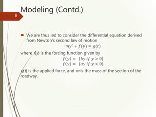
The document summarizes a study analyzing the collapse of the Tacoma Narrows Suspension Bridge in 1940. The objectives were to model the collapse mathematically and simulate it in Matlab. The model treats the bridge cables as springs with different stiffness in tension and compression. The simulation shows the amplitude of oscillations increasing over time, contradicting the traditional explanation of resonance causing collapse. It concludes the large oscillations were not due to resonance.

1. Group Members:
Muhammad Shan Saleem
Muhammad Ayaz
1

2. Objectives:
 To design a mathematical model for the collapse of Tacoma
bridge and analyze its cause.
 To simulate the system in Matlab and analyze the waveform
results.
2

3. Introduction
 In the summer of 1940, the Tacoma Narrows Suspension Bridge in
the State of Washington was completed and opened to traffic.
 Almost immediately, observers noticed that the wind blowing across
the roadway would sometimes set up large vertical vibrations in the
roadbed.
 Finally, on November 7, 1940, during a powerful storm, the
oscillations increased beyond any previously observed, and the
bridge was evacuated.
3

4. Introduction (Contd.)
 The entire span was eventually shaken apart by the large vibrations,
and the bridge collapsed.
4

5. Possible Cause ???
 The noted engineer von Karman was asked to determine the cause of
the collapse.
 He claimed that the wind blowing across the roadway separated into
vortices (wind swirls) alternately above and below the roadbed,
thereby setting up a periodic, vertical force acting on the bridge.
 It was this force that caused the oscillations.
5

6. Possible Cause (Contd.)
 Others further hypothesized that the frequency of this forcing
function exactly matched the natural frequency of the bridge,
thus leading to resonance, large oscillations, and destruction.
 For almost fifty years, resonance was blamed as the cause of
the collapse of the bridge
 Although the von Karman group denied this, stating that “it is
very improbable that resonance with alternating vortices plays
an important role in the oscillations of suspension bridges”
6

7. Mathematical Modeling
 Consider a single vertical cable of the suspension bridge.
We assume that it acts like a spring, but with different
characteristics in tension and compression, and with no
damping.
 When stretched, the cable acts like a spring with Hooke’s
constant, b, while, when compressed, it acts like a spring
with a different Hooke’s constant, a.
 We assume that the cable in compression exerts a smaller
force on the roadway than when stretched the same
distance.
7

8. Modeling (Contd.)
 We are thus led to consider the differential equation derived
from Newton’s second law of motion
𝑚𝑦" + 𝑓(𝑦) = 𝑔(𝑡)
where f(y) is the forcing function given by
𝑓 𝑦 = 𝑏𝑦 𝑖𝑓 𝑦 > 0
𝑓 𝑦 = {𝑎𝑦 𝑖𝑓 𝑦 < 0}
g(t) is the applied force, and m is the mass of the section of the
roadway.
8

9. Modeling (Contd.)
 We will assume that m= 1 kg, b= 4 N/m, a=1N/m, and g(t) =
sin(4t) N
 Therefore we must solve initial value problem
𝑦" + 4𝑦 = sin 4𝑡 𝑦(0) = 0; 𝑦′(0) = 0.01
 After solving above problem, we get the following solution
𝑦 𝑡 = sin 2𝑡 [
1
2
0.01 +
1
3
−
1
6
cos 2𝑡 ]
 We note that the first positive value of t for which y(t) is again
equal to zero is 𝑡 = 𝝅/2, so above equation holds on [0, 𝝅/2]
9

10. Modeling (Contd.)
 After t=𝝅/2, y becomes negative, so we must now solve the new
problem
𝑦" + 𝑦 = sin 4𝑡 𝑦(𝝅/2) = 0; 𝑦′(𝝅/2) = −(0.01 + 2/3)
 Proceeding as previous, the solution of above problem is
𝑦 𝑡 = cos 𝑡[ 0.01 +
2
5
−
4
15
sin 𝑡 cos 2𝑡]
 We note that the first positive value of t for which y(t) is again equal
to zero is 𝑡 = 3𝝅/2, so above equation holds on [0, 3𝝅/2]
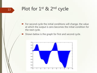
 Here our first cycle is completed, for next cycles the derived
problems will remain same but the initial conditions will change,
 The first value at which the system is equal to zero is our initial
conditions for next interval.
10

11. Simulation
 The whole model is implemented and simulated in Matlab
script.
 Solutions of initial value problems derived using
mathematical modeling is obtained by implementation of
2nd order differential equations in Matlab.
 Results obtained are then plotted in their respected
intervals.
 Detailed calculations are also performed by hand and is
attached with report.
11

12. Plot for 1st cycle
 For 0 to 𝝅/2 the derived initial value problem was
𝑦" + 4𝑦 = sin 4𝑡 𝑦(0) = 0; 𝑦′(0) = 0.01
 For 𝝅/2 to 3𝝅/2 the derived initial value problem was
𝑦" + 𝑦 = sin 4𝑡 𝑦(𝝅/2) = 0; 𝑦′(𝝅/2) = −(0.01 + 2/3)
Plotting graphs in Matlab
12

13. Plot for 1st & 2nd cycle
 For second cycle the initial conditions will change, the value
at which the output is zero becomes the initial condition for
the next cycle.
 Shown below is the graph for first and second cycle.
13

14. Results
 It is not surprising then that the amplitude of oscillations
will increase over time,
 Since the amplitude of (one term in) the solution during any
one cycle is directly related to the velocity at the beginning
of the cycle.
 It should be clear at this point that the large oscillations
causing the destruction of the Tacoma Narrows Suspension
Bridge were not the result of resonance.
14

15. References
 1. Lewis, G. N., “Tacoma Narrows Suspension Bridge Collapse” in A First Course in
Differential Equations, Dennis G. Zill, 253–256. Boston: PWS-Kent, 1993.
 2. Braun, M., Differential Equations and Their Applications, 167–169. New
York:Springer-Verlag, 1978.
 3. Amman, O. H., T. von Karman, and G. B. Woodruff, The Failure of the Tacoma
Narrows Bridge. Washington D.C.: Federal Works Agency, 1941.
 4. Lazer, A. C., and P. J. McKenna. Large amplitude periodic oscillations in
suspension bridges: Some new connections with nonlinear analysis. SIAM Review
32 (December 1990): 537–578.
 5. Peterson, I., Rock and roll bridge. Science News 137 (1991): 344–346.
 6. McKenna, P. J., Large torsional oscillations in suspension bridges revisited: Fixing
an old approximation. American Mathematical Monthly 106 (1999):1–18.
15