Downloaded 25 times
![Research Journal of Finance and Accounting www.iiste.org
ISSN 2222-1697 (Paper) ISSN 2222-2847 (Online)
Vol 3, No 8, 2012
2. Methodology
We address the issue of time series stationarity e.g unit root testing, co integration (long run relationship) and
presence of structural break. Structural change is an important problem in time series and affects all the inferential
procedures. A structural break in the deterministic trend will lead to misleading conclusion that there is a unit root,
when in fact there might be not.
In order to find the long term relationship (co integration) we apply the co integration technique of EG-model (1979).
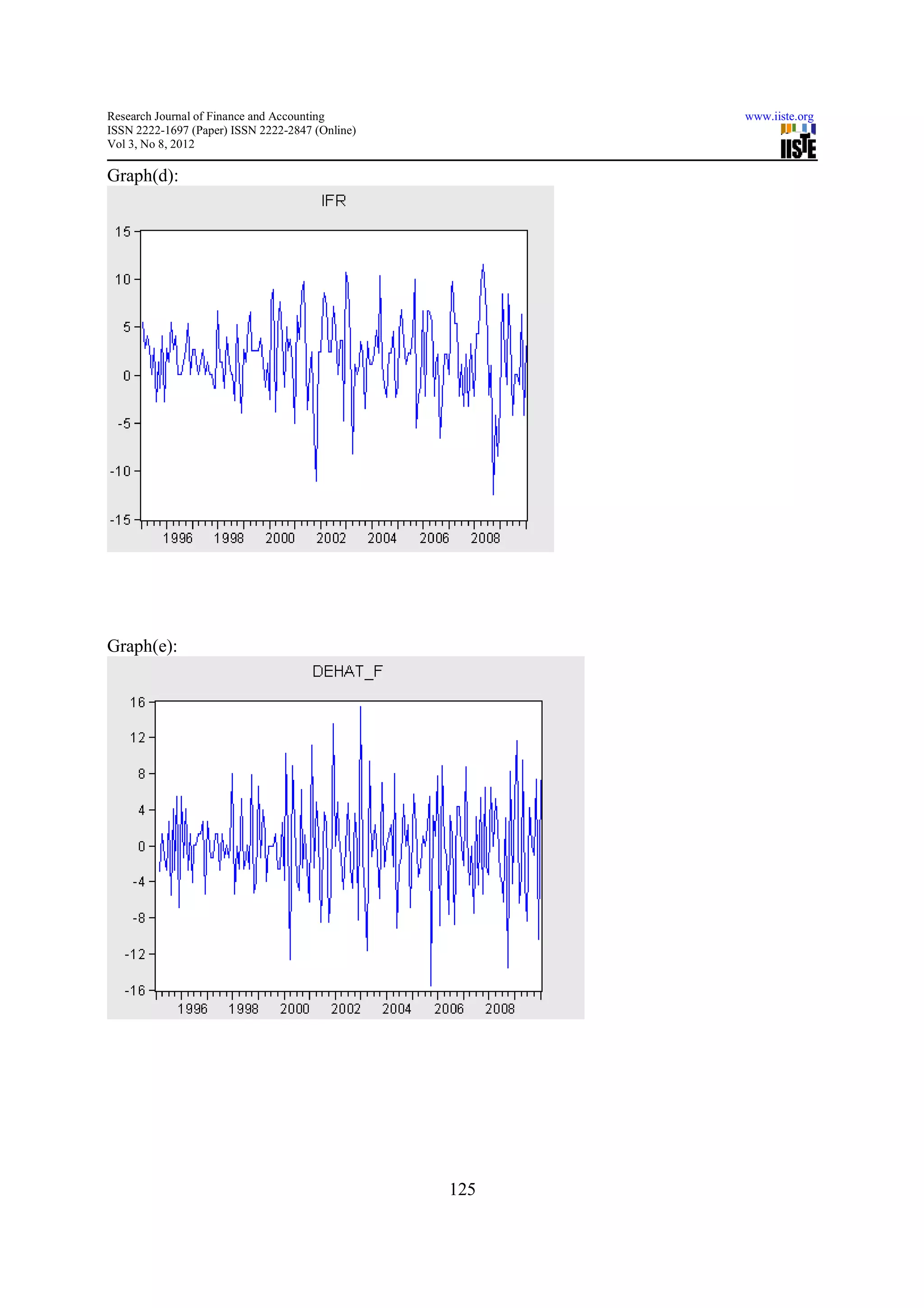
Further, we test the stationary and integration in TAR and MTAR. Generally for analysis, Firstly, we need to plot the
series and identify the presence of deterministic trends, secondly, we need to detrend the series and obtain the filtered
series, which are fluctuations around zero-horizontal line. Thirdly, we need to define the Heaviside function and
Estimate the specific model defined, then testing the related hypothesis. Finally, we need to test for deepness and
steepness asymmetric root for TAR and MTAR specification.
We collect the time series data of Canada from www.rba.gov.au . We generate the yearly inflation series from CPI
data by applying the formula.
Inflation= (CPI Current-CPI last/CPI Last)*4 (1)
Real Interest rate=Inflation-Interest rate (2)
2.1-Test for integration
We follow the following steps for it.
Consider a AR (1) model;
Yt= Yt-1+et
Case1-if |ф|<1 the series is stationary.
Case2-if|ф|>1 the series is non-stationary and explodes.
Case3-if|ф|=1 series contain a unit root and non-stationary.
A test for the order of integration is a test for the number of unit roots; it follows the step as under:
Step (a) - we Test “Yt” series if it is stationary then Yt is I(0). If No then Yt is I (n); n>0.
Step (b) - we Take first difference of Yt series as ∆yt=yt-yt-1 and test ∆yt to see if it is stationary.
If yes then yt is I (1); if no then yt is I (n); n>0 and so on.
2.2 TAR& MTAR Models Specification
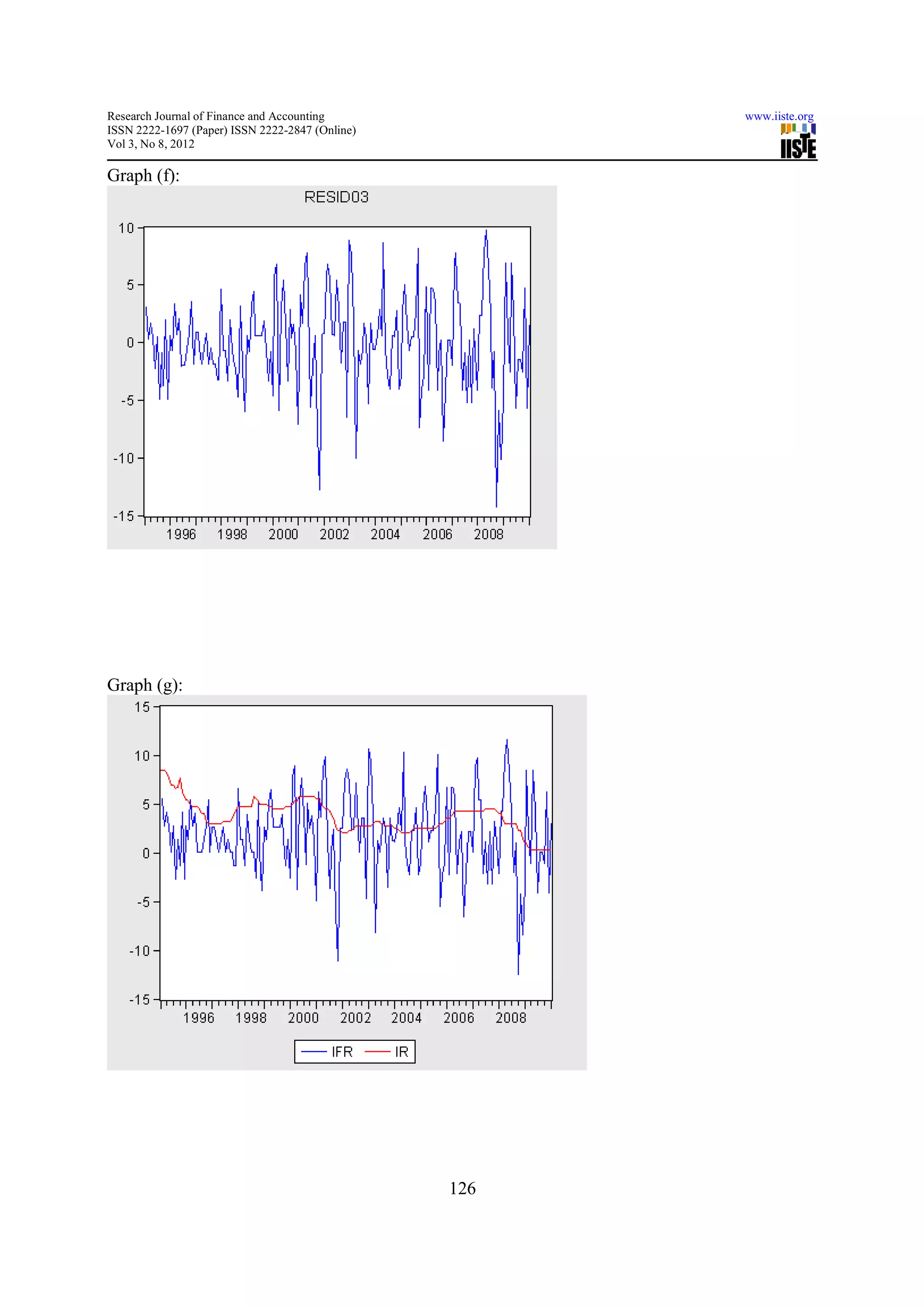
We detrend the series first and obtain the filtered series residuals. Define the Heaviside Indicator and decompose the
series in positive and negative. Estimate the models for testing the asymmetric unit root under the Null .We used
Enger and Granger (1998) critical values against F-statistics tabulated in order to draw the conclusion.
2.2.1- Testing for evidence of threshold stationarity
Actually when we conduct testing under TAR or MTAR model, the threshold parameter is unknown .We follow the
following steps to estimate the threshold parameters;
(a): define the first-differenced series: ∆yt=yt-yt-1
(b): making the series ∆yt sorted in ascending order
(c ): taking off 15% largest values and 15% smallest values.
(d): using remaining 70% values to estimate threshold parameters.
(e): estimate model ∆yt=It P1yt-1+(1-It)P2yt-1+et
For each possible threshold parameter, we find the lowest AIC, it is best estimate of threshold parameter.
To test yt is stationary or non-stationary: we do the following procedure:
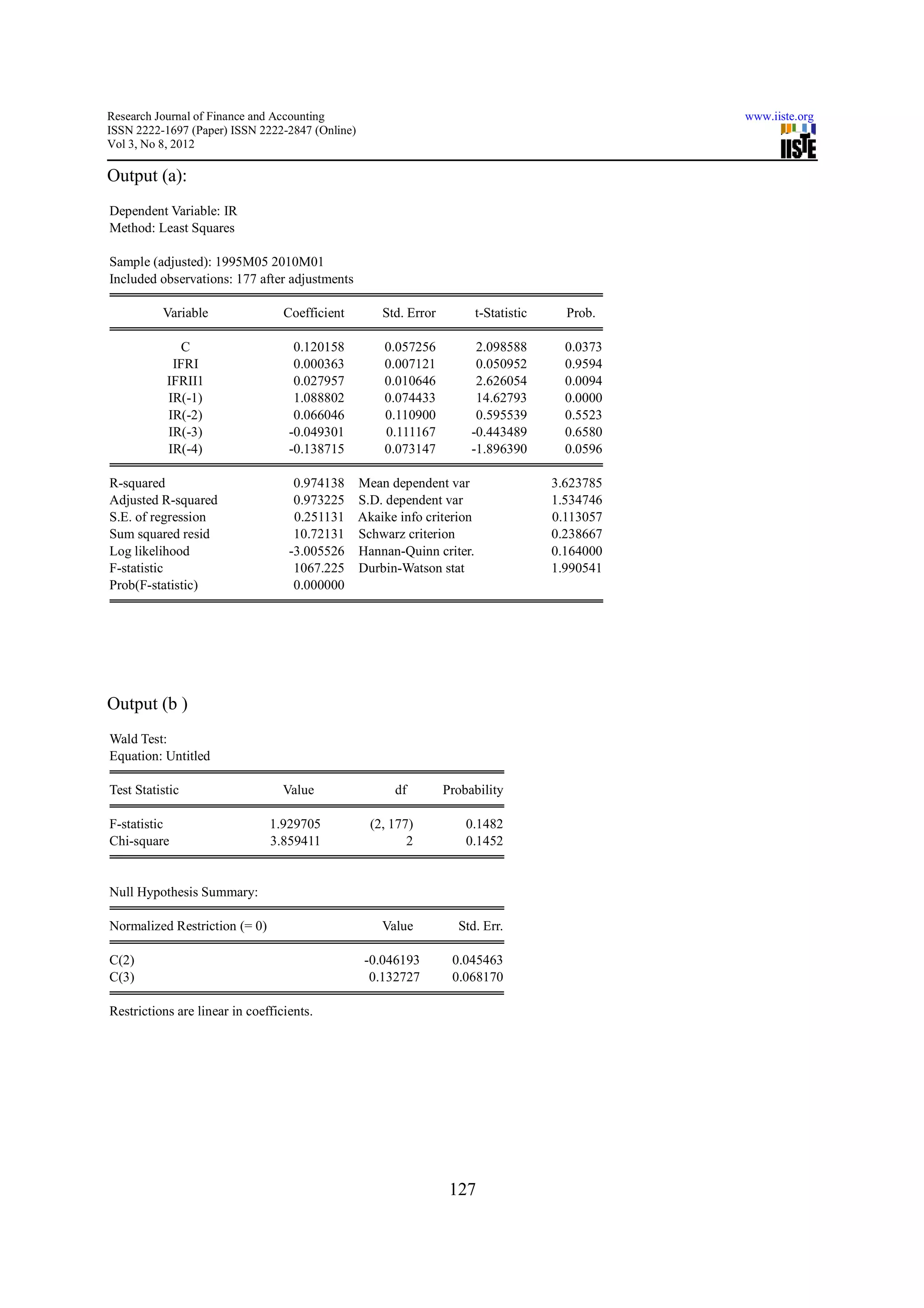
H0: P1=P2=0
H1:P1<0 and P2<0
Construct F=[(SSER-SSEUR)/J]/[SSEUR/(N-K)) (4)
If this value is larger than critical value then null hypothesis is rejected, series is stationary. Then we can test
steepness asymmetric roots as:
H0a: P1=P2
H1a: P1≠P2
Estimate model under H0a and H1a.
Construct F=[(SSER-SSEUR)/J]/[SSEUR/(N-K))
120](https://image.slidesharecdn.com/thresholdautoregressivetarmomentumthresholdautoregressivemtarmodelsspecification-121009022946-phpapp01/75/Threshold-autoregressive-tar-momentum-threshold-autoregressive-mtar-models-specification-2-2048.jpg)

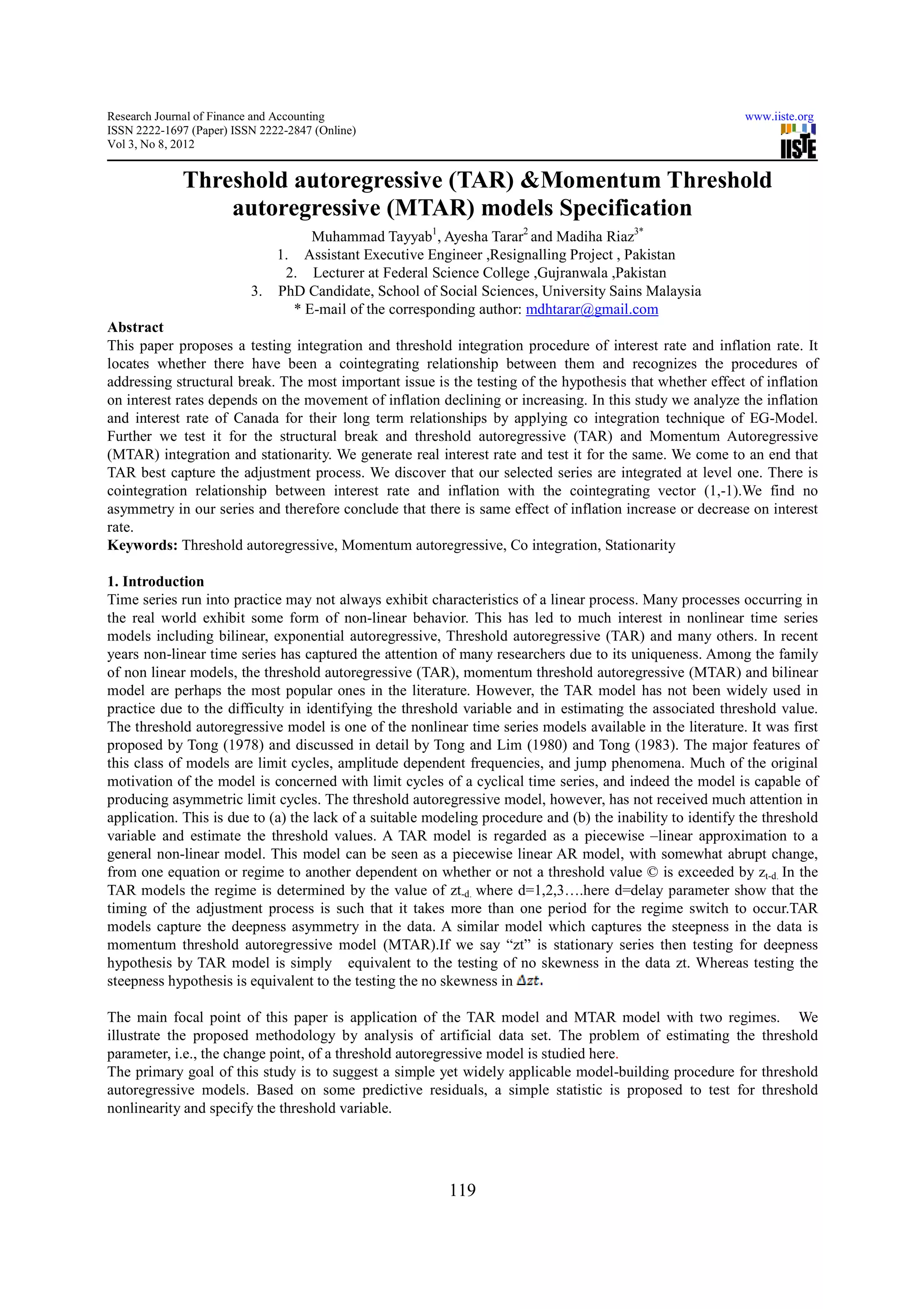
This paper proposes testing for integration and threshold integration between interest rates and inflation rates. It examines whether there is a cointegrating relationship between the variables and addresses issues of structural breaks. The paper analyzes inflation and interest rates in Canada using cointegration, threshold autoregressive (TAR), and momentum threshold autoregressive (MTAR) models to test for nonlinear relationships. The results show the variables are integrated at level one, there is cointegration between interest rates and inflation, and the TAR model best captures the adjustment process. No asymmetry is found, indicating inflation increases and decreases have the same effect on interest rates.