1. Uniwersytet Wrocławski
Wydział Matematyki i Informatyki
Instytut Matematyczny
Grzegorz Łoś
Pricing Exotic Options using Monte Carlo methods
Master’s thesis
written under the supervision of
Dr Paweł Kawa
Wrocław 2013
2. Oświadczam, że pracę magisterską wykonałem samodzielnie
i zgłaszam ją do oceny.
Data:.................... Podpis autora pracy:.........................
Oświadczam, że praca jest gotowa do oceny przez recenzenta.
Data:.................... Podpis opiekuna pracy:.........................
5. Abstract
This thesis presents techniques of option pricing based on Monte Carlo simulations. Mathemat-
ical theories underlying the presented methods are recalled, however, the thesis is practical in
its nature, hence intentionally it does not always get deep into mathematical details. I do not
consider myself as an author of any new proofs of commonly known theorems, but I attempted
to formulate and sketch key (even if sometimes not difficult) reasonings, so browsing through
this thesis could be beneficial even for people who are not engaged in academic mathematics,
but use it in their every day work (e.g. quants). Instead, it provides many algorithms in the
form of a concise pseudocode, which outline how to use the theory in practice. The utility of
depicted methods is affirmed by implementations in R and Java programming languages. This
paper is filled with illustrations of the results obtained by the created application.
The first chapter of the thesis gathers a group of definitions and facts from the probability
theory which are essential for the thesis, like Itˆo’s lemma, Girsanov theorem, a general description
of Monte Carlo methods. I begin with crude Monte Carlo method, because of its intuitiveness
and simplicity. I estimate the accuracy of this method, that is I derive a formula for dependency
between the number of simulations and the error of the estimation. Afterwards I describe two
variance reduction techniques used widely in practice – antithetic variates method and control
variates method. In Example 1.5 I compare these methods in a concrete application, which
shows how easily we can benefit by using the variance reduction. Paragraph 1.2.4 is devoted to
a practical problem of generating correlated pseudorandom values from the normal distribution
in a way available in most computational environments. Although the recalled algorithm is
presented in a n-dimensional context, I mostly focus on a 2-dimensional case. The experience
shows indeed, that this case appears most often in the quant’s practice.
In the second part, Reader may find an introduction to option pricing. It contains a descrip-
tion of the market model, the Black-Scholes paradigm, a definition of the martingale measure. It
also provides a detailed explanation how to calibrate parameters of the Black-Scholes model from
the real-world market’s history. Later, in section 6.6, the presented method is used to calibrate
the model for pricing options on a real-world assets. The second chapter also gathers definitions
of instruments which appear in practice most often. At first, simple vanilla options are described,
but more complicated derivatives, like barrier, Asian or basket options, are introduced as well.
In the next chapter, I describe the Monte Carlo pricing procedure for European options. I
start that part by applying the variance reduction techniques, described in chapter I, to price
instruments with European exercise. Consistent with the spirit of the whole thesis, I present
concrete valuations and analysis of the result stability on examples based on the real-life practice.
5
6. 6 Contents
I gradually move to more complicated exotic instruments, at first to those derivatives, whose
payoff may depend on on the whole history of the market scenario. At this point the superiority
of Monte Carlo methods over binomial trees, commonly used by economists, is clearly seen. For
instance, an attempt to use a binomial tree to price an Asian option expiring after one year would
require analysis of more than 1075 paths. Assuming that all present computers were combined in
one extremely powerful cluster, and that cluster was processing this particular pricing task since
the beginning of the universe, the humanity still would not have the valuation result.On the other
hand, the Monte Carlo method gives the price with a satisfactory accuracy in seconds. The next
kind of instruments described in the third chapter are basket options, whose payoff depends
on several assets. As previously, I illustrate this matter by concrete examples and I provide
pseudocodes, which may be easily implemented by the Reader. To the thesis I enclose a Java
application which uses implementations of these pseudocodes in an object oriented paradigm.
The fourth chapter introduces American contracts and collects several facts necessary to
value instruments with American-style exercise. A technique known as Least Squares Monte
Carlo or Longstaff-Schwartz method (LSM), which may be used to price American options, is
described. This technique is very desirable, due to the possibility to valuate a vast class of
American derivatives. However, it is unattainable for practicians who do not have a sufficient
mathematical background. In this chapter I strive to explain in the maximum extent the idea
behind the LSM method (especially in the context of difficulties occurring during naive attempts
to price American contracts using Monte Carlo methods). Afterwards I present a concrete step by
step example of the algorithm’s operation. After discoverers of the LSM, I quote two propositions
showing the correctness of the algorithm. In the last section I discuss the adjustments to LSM
allowing to price several types of exotic instruments.
The next part depicts an application which was created as an indispensable part of the thesis.
The application allows its users to price miscellaneous instruments via a user-friendly GUI. The
most important part of the program is a financial Java library, whose architecture is described
in the fifth chapter. The library bases on pseudocodes appearing in the paper, however, it was
adjusted to the object oriented programming language. I present the structure of the designed
classes in a form of UML diagrams. Of course, I focus only on the most important elements, i.e.
on these classes which correspond to topics discussed in the thesis, because the whole application
has about 200 classes and 30000 lines of code. Every concrete instrument, like a bond or an
option, has its own corresponding class, which derives from an interface representing an abstract
instrument. In order to implement the instrument hierarchy, the decorator pattern was used,
what allows to represent very exotic options without a necessity to create an additional class for
such an instrument. In the library there are also classes related to the algorithms described in
the thesis. Classes corresponding to crude Monte Carlo, antithetic variates and control variates
have a common base. Here, the template method pattern is involved – the pricing procedure is
implemented in the base class, however, it uses functionalities which have to be implemented in
the derived classes.
The last chapter shows capabilities of the created financial library. It gathers illustrations
of pricing results of several more complex instruments. Clearly, the application gives great
possibilities, therefore, it may be used by either practicians and academic community.
7. I
Preliminaries
There exists several approaches to the analysis of assets’ prices, for example fundamental anal-
ysis, technical analysis and quantitative analysis. Mathematicians are interested in the last one,
in which every asset is considered to be a stochastic process. Despite the fact that nobody
really believes that movements of asset prices are truly random, markets’ stochastic models are
commonly used, due to very satisfactory results. However, this approach requires non-trivial
mathematical background whose essentials are collected in this part.
1.1 Elements of stochastic analysis
We expect from Reader some basic knowledge of the probability theory and stochastic processes.
Purpose of this section is to recall definitions and facts essential for this work and to establish
notation.
Definition 1.1. Let (Ω, F, P ) be a probability space, (E, E) be a measurable space and T be a
positive real number. A stochastic process with values in a measurable space E, indexed by
an interval [0, T], is a family of random variables X = (Xt)T
t=0, where each Xt is E-valued.
For given ω ∈ Ω a trajectory of process X is a function t → Xt(ω), with domain T and
codomain E.
Remark 1.1. Stochastic process may be seen as a function X : Ω → ET . Then a trajectory is a
value of such function, i.e. for given ω, X(ω) is a trajectory. In the other words, a stochastic
process is a random function and a trajectory is its concrete realization.
Remark 1.2. In our applications space E always equals R or Rn.
Definition 1.2. A Brownian motion (or a Wiener process) is a stochastic process (Wt)t≥0
defined by following conditions:
• W0 = 0 a.s.,
• for any t, Wt ∼ N(0, t),
7
8. 8 1. Preliminaries
• increments of W are independent (i.e. for any t0 ≤ t1 ≤ . . . ≤ tn random variables
Wt0 , Wt1 − Wt0 , . . . , Wtn − Wtn−1 are independent,
• increments of W are stationary (i.e. for every 0 ≤ s < t, Wt − Ws is equal in distribution
to Wt−s),
• trajectories of W are continuous a.s.
In this thesis W always denotes the Brownian motion.
Definition 1.3. Filtration (Ft)T
t=0 on the probability space (Ω, F, P) is an increasing family
of σ-algebras contained in F, i.e. for all s < t, Fs ⊆ Ft ⊆ F.
Sometimes Ft is interpreted as a set of all events observable up to time t.
Definition 1.4. Process X = (Xt)T
t=0 is called adapted with respect to the filtration Ft if and
only if for all t ∈ [0, T], Xt is Ft-measurable.
Minimal filtration to which X is adapted is of course filtration generated by X, called natural
filtration, defined as FX
t = σ(Xs : s ≤ t).
Definition 1.5. A stopping time with respect to the filtration (Ft)T
t=0 is a random variable
τ : Ω → [0, T] ∪ {∞}, such that {τ ≤ t} ∈ Ft for all t ∈ [0, T].
If X is a process corresponding to some risky game, then a stopping time may be seen as a
strategy which tells us whether we should withdraw at time t, basing only on the information
accessible at time t.
Example 1.1. A typical example of a stopping time is first t, when Xt reaches a fixed barrier,
i.e.
τ = inf{t ∈ [0, T] : Xt ≥ b}
♦
Stopping times play important role in the financial mathematics. Often we are interested in
finding an optimal strategy for exercising an American option. Such strategy is a stopping time.
Definition 1.6. We call a stochastic process M = (Mt)T
t=0 a martingale with respect to the
filtration (Ft)T
t=0 if and only if it satisfies following conditions:
• for all t ∈ [0, T], Mt is Ft-measurable,
• for all t ∈ [0, T], E|Mt| < ∞,
• for all 0 ≤ s < t ≤ T, E[Mt|Fs] = Ms a.s.
Example 1.2. Brownian motion W is a martingale with respect to its natural filtration F.
Indeed, for all t > s we have
• Wt ∼ Ft,
• E|Wt| ≤
√
t < ∞ (because from Jensen’s inequality: (E|Wt|)2 ≤ EW2
t = t),
• E[Wt|Fs] = E[Wt − Ws|Fs] + E[Ws|Fs] = E[Wt − Ws] + Ws = Ws.
♦
9. 1.1. Elements of stochastic analysis 9
Example 1.3. Process (W2
t − t)t is a martingale with respect to W’s natural filtration F. Of
course (W2
t − t) ∼ Ft. From
E|W2
t − t| ≤ E(|W2
t | + |t|) = E(W2
t + t) = 2t
we have E|W2
t − t| < ∞. Moreover, for any t > s
E[W2
t − t|Fs] = E[(Wt − Ws)2
+ 2WtWs − W2
s |Fs] − t =
= E[(Wt − Ws)2
|Fs] + E[2WtWs|Fs] − E[W2
s |Fs] − t =
= E[(Wt − Ws)2
] + 2WsE[Wt|Fs] − W2
s − t =
= E[(Wt − Ws)2
] + 2W2
s − W2
s − t = W2
s − s.
♦
Definition 1.7. A stochastic process M = (Mt)T
t=0 is called a supermartingale with respect
to the filtration (Ft)T
t=0 if and only if it satisfies following conditions:
• for all t ∈ [0, T], Mt is Ft-measurable,
• for all t ∈ [0, T], E|Mt| < ∞,
• for all 0 ≤ s < t ≤ T, Ms ≥ E[Mt|Fs] a.s.
M is called a submartingale if it is satisfies the above conditions, but with an inequality
Ms ≤ E[Mt|Fs].
Example 1.4. For 0 ≤ s < t ≤ T we have
E[W2
t |Fs] > E[W2
t |Fs] − t + s = E[W2
t − t|Fs] + s = W2
s ,
hence W2
t is a submartingale. ♦
The breakthrough which initiated a rapid development of the financial mathematics was the
discovery of Itˆo integral, named after Japanese mathematician Kiyoshi Itˆo. We do not discuss
construction of such integral, what is done for example in [3]. Instead we provide some intuition
about its meaning. Itˆo integral of X = (X)T
t=0 with respect to Wiener process W = (W)T
t=0 is
a stochastic process
t
0
XsdWs
T
t=0
,
where
t
0
XsdWs = lim
n→∞
n
i=1
Xti−1 (Wti − Wti−1 ). (1.1)
10. 10 1. Preliminaries
and for each n, {ti}n
i=0 is a partition of the interval [0, t], whose diameter converges to 0 as n
tends to infinity. As we can see Itˆo integral is similar to the Stieltjes integral, which is defined
for g with locally bounded variation, and continuous f, as
t
0
f(s)dg(s) = lim
n→∞
n
i=1
f(ti−1)(g(ti) − g(ti−1)).
However, on almost all trajectories W has locally unbounded variation. In order to give sense
to equation (1.1), the limit has to be taken in L2.
Remark 1.3. Note that
• to integrate
t
0
Xsds we need only “standard” Riemann theory. The integrand is random,
but
t
0
Xsds can be treated as a function ω →
t
0
Xs(ω)ds and the last term is a Riemann
integral of a function X(ω).
•
t
0
XsdWs denotes a stochastic integral, thus its calculation requires Itˆo theory.
Definition 1.8. Let µ, σ ∈ C1, ξ be a Fs-measurable random variable. We say that process
X = (Xt)T
t=0 solves a stochastic differential equation (SDE)
dXt = µ(Xt)dt + σ(Xt)dWt,
X0 = ξ
if and only if
Xt = ξ +
t
0
µ(Xs)ds +
t
0
σ(Xs)dWs
for all t ∈ [0, T).
Remark 1.4. Sometimes indices are omitted and SDE is written in the form
dX = µ(X)dt + σ(X)dW.
Next definition presents one of the most important type of processes, used to model asset
movements in real-world markets.
Definition 1.9. A stochastic process S given by SDE
dSt = µStdt + σStdWt, (1.2)
where µ, σ ∈ R is called a geometric Brownian motion.
Now we can formulate a version of Itˆo’s lemma, which is widely used in financial mathematics.
11. 1.1. Elements of stochastic analysis 11
Theorem 1.1 (Itˆo’s lemma). Let S be a geometric Brownian motion as in (1.2), F : R2 →
R, F ∈ C2. Then
F(St, t) = F(S0, 0) +
t
0
∂F
∂S
(Sr, r)dSr +
t
0
∂F
∂t
(Sr, r)dr +
1
2
σ2
S2
t
t
0
∂2F
∂S2
(Sr, r)dr
or equivalently in SDE form
dF(St, t) =
∂F
∂S
(St, t)dSt +
∂F
∂t
(St, t)dt +
1
2
σ2
S2
t
∂2F
∂S2
(St, t)dt. (1.3)
In the books on the stochastic processes Itˆo’s lemma is proven in much greater generality.
However, for our purposes, as in many other literature on financial mathematics, the formulated
theorem is sufficient. Equation (1.3) is also called an Itˆo’s formula.
Itˆo’s lemma is a very powerful tool, indispensable in Black-Scholes theory. We show how it
can be used to solve equation (1.2).
Proposition 1.2. Let S be a geometric Brownian motion, as in (1.2). Solution of its SDE is
given by
St = S0 exp (µ −
1
2
σ2
)t + σWt . (1.4)
Proof. We apply Itˆo’s formula with F(S, t) = ln(S). We have
dF =
∂F
∂S
dS +
∂F
∂t
dt +
1
2
σ2
S2 ∂2F
∂S2
dt
=
∂F
∂S
(µSdt + σSdW) +
∂F
∂t
dt +
1
2
σ2
S2 ∂2F
∂S2
dt
=
1
S
(µSdt + σSdW) + 0dt −
1
2
σ2
S2 1
S2
dt
= (µ −
1
2
σ2
)dt + σdW
.
From Definition 1.8
F(St, t) = F0 +
t
0
(µ −
1
2
σ2
)ds +
t
0
σdWs
= F0 + (µ −
1
2
σ2
)t + σWt.
.
By substituting S0 = eF0 , we get
S = S0 exp (µ −
1
2
σ2
)t + σWt .
12. 12 1. Preliminaries
So far, we have discussed only one dimensional stochastic processes. However, often we
have to take into account several assets at once, thus we need mathematical tools to describe
multidimensional cases.
Definition 1.10. Process W is called d-dimensional standard Wiener process if it is a
vector process (its values are in Rd) of the form
W =
W(1)
W(2)
...
W(d)
,
where all components are independent Wiener processes.
Movements of asset prices usually cannot be regarded as independent. We need notation to
describe dependency between processes.
Definition 1.11. We say that Wiener processes W and V are correlated and have correlation
, what we denote by
Corr(W, V ) = ,
if and only if
Corr(W1, V1) = .
Remark 1.5. It is easy to notice that Corr(W1, V1) = if and only if for all t > 0, Corr(Wt, Vt) =
.
Definition 1.12. The process W is called d-dimensional correlated Wiener process with
correlation matrix Σ = ( ij)d
i,j=1, if and only if W = [W(1), W(2), . . . , W(d)] , where for each i, j,
Corr(W(i), W(j)) = ij.
We end this section with the Girsanov theorem, whose significance in the financial mathe-
matics arises from the fact, that it allows us to move from the real measure P to an equivalent
martingale measure P∗ . In the literature exist many versions of this theorem. The one presented
here comes from [1], there Reader may also find the proof.
Theorem 1.3 (Girsanov theorem). Let ¯W be a d-dimensional standard Wiener process on
the probability space (Ω, F, (Ft)T
t=0, P ) and let ϕ be any d-dimensional adapted column vector
process. Choose a fixed T and define the process L on [0, T] by
Lt = exp
t
0
ϕs · d ¯Ws −
1
2
t
0
||ϕs||2
ds.
Assume that
EP
[LT ] = 1,
13. 1.2. Introduction to Monte Carlo methods 13
and define the new probability measure Q on FT by
dQ
dP
= LT , on FT .
Then W given by
Wt = ¯Wt −
t
0
ϕsds
is a standard Wiener process under Q.
Remark 1.6. Symbol · in definition of L is the inner product of two vectors.
1.2 Introduction to Monte Carlo methods
Monte Carlo methods are a class of algorithms designed for estimation of unknown values by
simulation. They do not refer to any particular algorithm, they are rather a general “recipe”
for procedures, which obtain results by simulation.
1.2.1 Crude Monte Carlo
Suppose that we want to estimate an unknown value I, which can be written as expected value
of some random variable, i.e.
I = EY. (1.5)
The idea of Monte Carlo technique is to replicate Y many times, and as an estimation of I take
an average. So
I ≈
1
n
n
i=1
Yi,
where n is a big natural number and Yi are independent, with the same distribution as Y .
This procedure is justified by the strong law of large numbers. Let
ˆY CMC
n =
1
n
n
i=1
Yi. (1.6)
Of course E ˆY CMC
n = EY = I, so ˆY CMC
n is unbiased. Moreover, from the law of large numbers
ˆY CMC
n −−−→
n→∞
I a.s., what explains why Monte Carlo method works.
Value ˆY CMC
n is called crude Monte Carlo (CMC) estimator. Simple calculation gives its
variance
Var( ˆY CMC
n ) =
1
n
Var(Y ). (1.7)
In this paragraph we simply write ˆYn instead of ˆY CMC
n .
Here appears a natural question, how big should be the number n to obtain the satisfying
accuracy of the estimator? To find an answer we have to specify the question a little more: for
14. 14 1. Preliminaries
chosen numbers b and α, how big should be n, so we could tell, that an error of the estimation,
with probability 1 − α, is not greater than b?
Let σ =
√
VarY , z1−α/2 = Φ−1(1 − α/2), where Φ is the cumulative distribution function of
the normal distribution. Strong convergence of ˆYn implies also weak convergence, what means
that
P (| ˆYn − I| > b) −−−→
n→∞
0 a.s.,
for any b > 0. Hence we write
P (−b ≤ ˆYn − I ≤ b) = 1 − α
P (−b ≤
n
i=1
Yi − nI
n
≤ b) = 1 − α
P (−
b
√
n
σ
≤
n
i=1
Yi − nI
√
nσ
≤
b
√
n
σ
) = 1 − α
From Central Limit Theorem we know that
lim
n→∞
P (−z1−α/2 ≤
n
i=1
Yi − nI
√
nσ
≤ z1−α/2) = 1 − α,
hence for large n we have
z1−α/2 ≈
b
√
n
σ
.
In a typical situation we do not know the variation of Y (we do not even know the expected
value, after all we are using Monte Carlo method to find it!), so the above formula has rather
theoretical meaning. Instead, we have to use an unbiased estimator
ˆσ =
1
n − 1
n
i=1
(Yi − ˆYn)2
and replace σ by ˆσ in above approximation. The foregoing discussion may be considered a sketch
of a proof of following
Theorem 1.4. Dependency between a number of simulations n, an error b and a confidence
level α is given by following formulas
b =
ˆσz1−α/2
√
n
(1.8)
n =
ˆσ2z2
1−α/2
b2
. (1.9)
15. 1.2. Introduction to Monte Carlo methods 15
Equation (1.8) tells us how big is an error of the estimation when we performed n simulations.
Equation (1.9) inverses the situation, it allows us to plan the number of simulations necessary
to obtain requested accuracy.
Unfortunately equation (1.8) tells us that convergence of the Monte Carlo method is slow. To
improve accuracy by one more digit, one have to perform 100 times more simulations. The only
way to decrease the number of necessary simulations is to choose Y with the smallest possible
variance. In next paragraphs, two methods of variance reduction are discussed.
The confidence level α, which appears in (1.8) in the quantile function, is not essential when
comparing two estimators. Hence we introduce
Definition 1.13. Value
ˆσ
√
n
(1.10)
is called standard error (abbreviated s.e.).
Suppose that in some fixed time we can take n samples from the distribution of Y , and m
samples from the distribution of Z, where EY = EZ = I. In order to settle which estimator is
better, ˆYn or ˆZm, it is sufficient to compare their standard errors, that is
ˆσY
√
n
and
ˆσZ
√
m
.
Since z0.975 ≈ 2, equation (1.8) tells us that with 95% confidence the difference between
the real value and the result of the estimation does not exceed two standard errors.
1.2.2 Antithetic variates
Let us consider again I and Y as in (1.5). Equation (1.9) shows that the number of simulations
required to obtain given accuracy is proportional to variance of Y . It explains the necessity of
choosing Y wisely. If we can find Y which has smaller variance than Y , then we can significantly
decrease the number of needed simulations. We describe two techniques of variance reduction:
this paragraph introduces antithetic variates method, and the following presents control variates
method.
In antithetic variates method (AV method) every sample is a pair of values, each from
the same distribution as Y . Every of n sample pairs is independent from each other, however
random variables in a pair should be correlated. In the other words we consider pairs (Y2i−1, Y2i),
i = 1, 2, ..., n, where each (Y2i−1, Y2i) is independent from (Y2j−1, Y2j), if i = j, and for some ,
Corr(Y2i−1, Y2i) = . Let
˜Yi =
Y2i−1 + Y2i
2
, i = 1, 2, ..., n.
It is clear that ( ˜Yi)n
i=1 are i.i.d., and their variance satisfies
Var( ˜Yi) =
1
4
Var(Y2i−1 + Y2i) =
1
4
(Var(Y2i−1) + Var(Y2i) + 2 · Cov(Y2i−1, Y2i))
=
1
4
(2 · Var(Y ) + 2 · Var(Y ) )
=
Var(Y )
2
(1 + ).
16. 16 1. Preliminaries
We define antithetic variates estimator as
ˆY AV
n =
1
n
n
i=1
˜Yi.
It is clear that such estimator is unbiased, i.e. E ˆY AV
n = I. Let us calculate its variance
Var( ˆY AV
n ) =
1
n2
Var(
n
i=1
˜Yi)
=
1
n
Var( ˜Yi) =
Var(Y )
2n
(1 + ).
(1.11)
In order to calculate ˆY AV
n we have to take 2n samples (or rather n pairs of samples). From (1.7)
we see that variance of the crude Monte Carlo estimator, which performs the same number of
draws, equals 1
2n Var(Y ). Hence, if correlation of random variables in a pair is negative, then we
reduce variance. In consequence the number of simulations necessary to keep an error smaller
than b, at the confidence level α is also smaller.
1.2.3 Control variates
The control variates method (CV method) also involves drawing pairs of values, however in
opposite to antithetic variates method, elements in pair do not come from the same distribution
and expected value of the second distribution must be known. More precisely, we consider pairs
(Yi, Xi), i = 1, 2, ..., n, where each (Yi, Xi) is independent from (Yj, Xj), if i = j, EX is known
and |Cov(Yi, Xi)| > 0. Let ˆXn = 1
n
n
i=1 Xi. Control variates estimator is defined as
ˆY CV
n = ˆY CMC
n + c( ˆXn − EX) (1.12)
for some c. Clearly, ˆY CV
n is unbiased. In order to reduce variance, c must be chosen properly.
We have
Var( ˆY CV
n ) = Var( ˆY CMC
n + c ˆXn) =
1
n2
Var
n
i=1
(Yi + cXi)
=
1
n
Var(Y + cX) =
1
n
(Var(Y ) + 2cCov(Y, X) + c2
Var(X)).
The last expression is a simple quadratic equation with respect to c, hence it is easy to determine
for which argument it reaches its minimum value:
c = −
Cov(Y, X)
Var(X)
.
Let = Corr(Y, X). By substituting c to the last equation we obtain
Var( ˆY CV
n ) =
1
n
Var(Y ) − 2
Cov(Y, X)2
Var(X)
+
Cov(Y, X)2
Var(X)2
Var(X)
=
1
n
Var(Y ) −
Cov(Y, X)2
Var(X)
=
Var(Y )
n
1 − 2
(1.13)
17. 1.2. Introduction to Monte Carlo methods 17
Crude Monte Carlo estimator, which takes the same number of random variables (i.e. 2 times the
number of pairs in control variates method) has the variance equal to Var(Y )
2n . Thus if 1 − 2 < 1
2
we reduce the variance.
In practice, however, we do not know values Var(X) (we only assumed we know expectation
of X) and Cov(Y, X). Hence in the simulations we have to use
c = −
σ2
XY
σ2
X
, (1.14)
where
σ2
XY =
1
n − 1
n
i=1
(Xi − ˆXn)(Yi − ˆY CMC
n ),
σ2
X =
1
n − 1
n
i=1
(Xi − ˆXn)2
.
Example 1.5. To compare presented Monte Carlo methods let us calculate value of I =
1
0 exdx by simulation. Of course exact value equals e − 1 ≈ 1.71828183. Let g(x) = ex and
U ∼ U(0, 1). Then
I = E[g(U)],
hence we can use derived theory with Y = g(U). We consider following estimators:
ˆY CMC
2n =
1
2n
2n
i=1
g(Ui),
ˆY AV
n =
1
n
n
i=1
g(Ui) + g(1 − Ui)
2
,
ˆY CV
n =
1
n
n
i=1
g(Ui) + c(Ui −
1
2
) ,
where c is as in (1.14) with Y = g(U) and X = U. Note that we are taking twice as much
simulations in crude Monte Carlo method, since it does not use pairs of random variables. The
results of comparison of all presented methods are gathered in Table 1.1 and Figure 1.1.
We see that in this case antithetic and control variates methods gave approximately equal
results, while crude Monte Carlo is far behind them. When performing one million simulations
(in case of CMC two millions) standard error turned out 50 times smaller in AV and CV than in
CMC. It means that results from the first two methods are more than one digit more accurate.
The box plot in Figure 1.1 shows that a variance of the crude Monte Carlo estimator is much
more greater than in the two other methods. In practice it means, that if we ran simulations
with AV estimator or CV estimator several time, then every time we would obtain more or less
equal result. For CMC the discrepancy between the results would be much greater. The lower
illustration explains that fact – convergence of CMC is definitely slower than two other methods.
18. 18 1. Preliminaries
Table 1.1: Results of calculating
1
0
ex
dx by simulation.
CMC AV CV
log10(n) ˆY CMC
2n s.e. ˆY AV
n s.e. ˆY CV
n s.e.
2 1.69825 0.03504 1.71717 0.00648 1.71962 0.00638
3 1.72458 0.01094 1.72171 0.00205 1.72032 0.00203
4 1.72116 0.00349 1.71805 0.00062 1.71918 0.00063
5 1.71665 0.00110 1.71802 0.00020 1.71844 0.00020
6 1.71796 0.00035 1.71831 0.00006 1.71829 0.00006
1.715
1.720
1.725
CMC AV CV
method
Estimatedvalue
method
AV
CMC
CV
1.715
1.720
1.725
0 25000 50000 75000 100000
replicated pairs
estimatedvalue
method
av
cmc
cv
Figure 1.1: The upper picture presents a “result cloud”. For each method 10000 simulations were run
100 times. Hence each method gave 100 estimations of
1
0
ex
dx. Small points indicate obtained values.
As usually in box plots, the lower and upper edges of the boxes are first and third quartiles. In the lower
picture we see the comparison of the speed of convergence.
19. 1.2. Introduction to Monte Carlo methods 19
In order to realize why AV and CV methods lead to so similar accuracy, look at (1.11) and
(1.13). In AV method variance is reduced by a coefficient
1 + Corr(eU , e1−U )
2
≈
1 − 0.968
2
= 0.0162,
while in CV method variance is reduced by a coefficient
1 − Corr(eU
, U)2
≈ 1 − 0.9922
= 0.0163.
Such similarity of the results is pure coincidence.
Let us finish this example with a remark that this was a preconceived case, which showed
that variance reduction techniques may be very useful. Actually, in many applications it may
be difficult to find appropriate pairs of highly correlated random variables necessary to use AV
or CV methods. ♦
1.2.4 Simulation
Now, when we know how Monte Carlo methods work, we need to describe how to get random
values.
Independent standard normal random variables. Most computational environments and
programming languages have built-in generator of values from uniform distribution. We show
how to obtain (pseudo)random variables with the ubiquitous normal distribution.
The most popular way is to use the Box-Muller transformation (Algorithm 1.1) which
uses two independent variates with the uniform distribution on (0, 1), and “produces” two in-
dependent variates with the standard normal distribution.
Algorithm 1.1 The Box-Muller method.
1: function BoxMuller()
2: Generate independent random variables U1, U2 ∼ U(0, 1),
3: Z1 ← −2 log(U1) cos(2πU2),
4: Z2 ← −2 log(U1) sin(2πU2),
5: return (Z1, Z2).
6: end function
This method returns values of two independent random variables coming from the standard
normal distribution. When we need more than two samples, then of course we repeat that
algorithm as many times as necessary.
In [4] we can find a remark that necessity of calculating sine and cosine may slow down the
above algorithm. Another method, polar rejection, is proposed (Algorithm 1.2). However,
conducted experiments do not show any significant difference in efficiency of both presented
methods. It brings us to the conclusion that the efficiency of both algorithms is comparable and
not worth bothering. Moreover, which method is faster may depend even on the choice of the
programming language.
20. 20 1. Preliminaries
Algorithm 1.2 Polar rejection method.
1: function PolarRejection(µ, σ)
2: Generate independent random variables U1, U2 ∼ U(0, 1),
3: V1 ← 2U1 − 1,
4: V2 ← 2U2 − 1,
5: W ← V 2
1 + V 2
2 ,
6: if W > 1 return to step 2.,
7: Z1 ← −2 log(W)
W V1,
8: Z2 ← −2 log(W)
W V2,
9: return (Z1, Z2).
10: end function
Independent non-standard normal random variables. Sampling from an arbitrary nor-
mal distribution N(µ, σ2) is now straightforward. From the elementary probability theory comes
the method presented in Algorithm 1.3.
Algorithm 1.3 Drawing a random variable from the normal distribution N(µ, σ2).
1: function GaussDistr()
2: (Z1, Z2) ← BoxMuller() or (Z1, Z2) ← PolarRejection()
3: return µ + σ · Z1
4: end function
Correlated normal random values. The above methods allow us to generate independent
random variables. In the real world, however, we notice dependencies between observed phe-
nomena. For example movements of prices of the market assets are usually correlated. When the
market is in a boom cycle, then all the prices are increasing; on the other hand, if the recession
comes, all of the prices are sinking down. In order to model such values we must be able to
generate correlated random variables.
Let us begin with two standard normal random variables with correlation . We want to
obtain N1, N3 ∼ N(0, 1) such that Corr(N1, N3) = . For now we can only generate independent
N1 and N2, i.e. Corr(N1, N2) = 0. On the other hand Corr(N1, N1) = 1. Here rises the idea
that there exists N3 of the form N3 = aN1 + bN2, such that Corr(N1, N3) = . It should come
from the standard normal distribution, thus
1 = Var(N3) = Var(aN1) + Var(bN2) = a2
+ b2
Moreover
= Corr(N1, N3) = Cov(N1, N3) = aCov(N1, N1) + bCov(N1, N2) = a
Hence
a = , b = 1 − 2.
We have proven following
21. 1.2. Introduction to Monte Carlo methods 21
−2
0
2
4
−2 0 2
Z1
Z2
−2
0
2
−2 0 2
Z1
Z2
−2
0
2
−2 0 2
Z1
Z2
−2
0
2
−2 0 2 4
Z1
Z2
Figure 1.2: Graphical illustration of the dependency between two normal correlated random variables
Z1 and Z2. In the upper left corner = −0.9, upper right: = −0.5, lower left: = 0 (independent
variables), lower right: = 0.5.
Proposition 1.5. If Z1 and Z2 are independent random variables with the same distribution
N(0, 1), then for any ∈ [−1, 1] random variables
N1 = Z1
N2 = Z1 + 1 − 2Z2
have distribution N(0, 1) and Corr(N1, N2) = .
Remark 1.7. Let Σ =
1
1
, and L =
1 0
1 − 2
. Clearly, vector N = (N1, N2)
from Proposition 1.5 has the Gaussian distribution N(0, Σ). Moreover, N = LZ. There is an
interesting correspondence between Σ and L – simple matrix multiplication shows that Σ = LL .
The derivation of the above fact was intuitive, but we need a more general version. It turns
out that Proposition 1.5 can be generalized for higher dimensions.
Theorem 1.6. For the positive-definite matrix Σ there exists a lower triangular matrix L, such
that Σ = LL . This representation of Σ is called the Cholesky decomposition.
Matrix L from the above theorem may be obtained by the Cholesky algorithm. Utility of
the Cholesky decomposition arises from the following fact.
Proposition 1.7. Let Z be a random vector with the multivariate normal distribution N(0, I).
Let Σ be a co variance matrix and Σ = LL . Then vector N = µ + LZ has the distribution
N(µ, Σ).
22. 22 1. Preliminaries
Proof. It is clear that N has the multivariate normal distribution. Moreover,
EN = E(µ + LZ) = µ + L · EZ = µ,
Cov(N) = E (N − EN)(N − EN) = E (LZ − L · EZ)(LZ − L · EZ) =
= E L(Z − EZ)(Z − EZ) L = L · E (Z − EZ)(Z − EZ) · L =
= L · Cov(Z) · L = LL = Σ.
That explains how works Algorithm 1.4 for generating values from the multivariate normal
distribution with given mean vector µ and positive-definite covariation matrix Σ.
1. Use Cholesky decomposition to obtain matrix L such that Σ = LLT ,
2. Using previously shown method generate vector N of independent random variables with
standard normal distribution.
3. Return µ + LN.
Algorithm 1.4 The polar rejection method.
1: function GaussMultiVariate(µ, Σ)
2: L ← CholeskyAlgorithm(Σ)
3: Z ← vector of independent standard normal random variables.
4: Z is obtained from BoxMuller or PolarRejection
5: return µ + Σ · Z
6: end function
23. II
Basics of option pricing
One of the main fields of interest in the financial mathematics is pricing so-called contingent
claims, which are financial instruments whose value depends on some other assets. In case of the
European options there exists a straightforward formula, derived by Black and Scholes in 1973,
which gives the option’s price. Another way of pricing is using Monte Carlo simulations. Al-
though the simulations are time-consuming and for that reason less effective than Black-Scholes
formula, they are widely used because of the possibility to adjust them to very sophisticated
contingent claims.
2.1 Elements of arbitrage theory
Mathematical approach to the analysis of assets’ prices requires modelling the prices as stochastic
processes. This section describes fundamental concepts. The notation and the description of
the market model presented here is based on [2].
2.1.1 Underlying framework
Throughout this thesis we assume we are given a probability space (Ω, F, (Ft)T
t=0, P ). Since it is
observed by investors, P is sometimes called a real measure, in opposite to an artificial risk-
neutral measure, which is later on. Elements of Ω are called market scenarios. Furthermore
σ-algebra Ft may be seen as a set of all events observable up to time t.
We consider a market with d + 1 assets, where each asset S(i) = (S
(i)
t )T
t=0 is modelled as a
R+-valued stochastic process adapted to (Ft)T
t=0. The 0th asset is the money stored in a locally
riskless bank account and is given by
S
(0)
t = exp
t
0
r(t)dt
,
where r(t) is a short term riskless interest rate at time t. In general r(t) may also be a stochastic
process, however, in this thesis we focus only on the case r(t) ≡ r and then S(0) may also be
23
24. 24 2. Basics of option pricing
regarded as a bond, paying erT at time T. By S we denote a d-dimensional (column) vector of
prices of the risky assets, i.e.
St = (S
(1)
t , S
(2)
t , . . . , S
(d)
t ) , 0 ≤ t ≤ T.
We also introduce notation ¯S for a (d + 1)-dimensional vector of prices of all assets, that is
¯St = (S
(0)
t , St) = (S
(0)
t , S
(1)
t , . . . , S
(d)
t ) , 0 ≤ t ≤ T.
For convenience we also consider discounted time processes
X
(i)
t =
S
(i)
t
S
(0)
t
.
It allows us to compare asset prices quoted at different times. In similar manner as previously
we use notation X, ¯X for vectors of the discounted prices,
Xt = (X
(1)
t , X
(2)
t , . . . , X
(d)
t ) , 0 ≤ t ≤ T.
¯Xt = (X
(0)
t , X
(1)
t , . . . , X
(d)
t ) , 0 ≤ t ≤ T.
Next definition gives us a notation to describe the content of portfolio.
Definition 2.1. A dynamic trading strategy is any Ft-adapted, Rd+1-valued process ¯ξ =
(¯ξt)T
t=0 = (ξ
(0)
t , ξt)T
t=0 = (ξ
(0)
t , ξ
(1)
t , . . . , ξ
(d)
t )T
t=0.
Each ξ
(i)
t has an interpretation of the quantity of shares of the ith asset held in portfolio
at time t (it may be negative, then it corresponds to the short sale). Thus, the notion of the
portfolio and the dynamic trading strategy may be equated. The value of the portfolio at time
t equals
¯ξt · ¯St =
d
i=0
ξ
(i)
t S
(i)
t ,
where · is the inner product of two vectors.
Assume that investor’s portfolio is worth 101,000$ today and a year ago it was worth
100,000$. When was the investor’s financial condition better, today or a year ago? If the
riskless interest rate equals 5%, then the investor would gain more if he put all his capital into
a bank account. This example shows the necessity of discounting to compare portfolios whose
values are quoted at different times.
Definition 2.2. The discounted value process V ξ = (V ξ
t )T
t=0 associated with a trading
strategy ¯ξ is given by
V ξ
t = ¯ξt · ¯Xt.
25. 2.1. Elements of arbitrage theory 25
2.1.2 Arbitrage opportunities
The value V ξ
0 is the initial investment into the portfolio. Following definition introduces port-
folios which do not receive cash flows from the “outside world” after initialization. They are
rearranged in such a way that purchases of new assets must be covered by selling some other
assets, so value of the portfolio before and after rearranging stays the same.
Definition 2.3. A dynamic trading strategy is called self-financing if and only if for every
0 ≤ t ≤ T
d
i=0
dξ
(i)
t (S
(i)
t + dS
(i)
t ) = 0.
This definition, although being very simple, looks completely incomprehensible at first sight.
To convey some intuition let us think that dt is a very small, even infinitesimal, time period.
Vector ¯ξt describes content of the portfolio at the beginning of the period. After time dt change
of the stock prices equals d ¯St. The portfolio needs a rearrangement – d¯ξt represents changes of
quantities of the held assets. Thus d¯ξt · ( ¯St + d ¯St) is the total cost of the rearrangement. From
the definition it equals 0, what explains the name self-financing.
From now on we consider only those market models that are efficient in the sense that they
are arbitrage-free.
Definition 2.4. An arbitrage opportunity is a self-financing portfolio ¯ξ, such that
V ξ
0 = 0
P (V ξ
T ≥ 0) = 1
P (V ξ
T > 0) > 0
The market is arbitrage-free if it does not allow for arbitrage opportunities.
What does arbitrage opportunity mean in practice? Assume an investor entering the market
without any capital. He builds his portfolio by short sale of some assets and purchase of other
assets for received money. Arbitrage opportunity is a situation when the investor at time T can
cover his short positions by sale of assets held long, and with positive probability he has some
remaining cash. In the other words, he can make money without exposure to any downside risk.
Now we are moving to an important concept of a martingale measure.
Definition 2.5. A probability measure P∗ is called a martingale measure (or a risk neutral
measure) if and only if the discounted price process X is a P∗ -martingale, i.e. for all 0 ≤ s ≤
t ≤ T
E∗
[Xt] < ∞ and E∗
[Xt|Fs] = Xs (2.1)
Remark 2.1. Condition (2.1) is written for a vector process X, hence for every 1 ≤ i ≤ d
E∗
[X
(i)
t ] < ∞ and E∗
[X
(i)
t |Fs] = X(i)
s
26. 26 2. Basics of option pricing
Let us recall that two measures P and P∗ defined on σ-algebra F are equivalent if and
only if for all A ∈ F, P (A) = 0 if and only if P∗ (A) = 0. Next theorem, known as the first
fundamental theorem of asset pricing, shows the importance of martingale measures.
Theorem 2.1 (First FTAP). The following to statements are essentially equivalent:
1. The market model is arbitrage free.
2. There exists martingale measure P∗ equivalent to P .
Unfortunately, due to an appearance of a word “essentially, this is rather a “meta-theorem”.
It can be given a sharp, mathematical sense – see for example Theorems 10.9 and 10.10 in [1].
In the discrete case, however, theorem holds without the word “essentially, as it is proven in [2]
(Theorem 5.17). This case is sufficient for us, since in Monte Carlo methods price trajectories
are simulated only in a finite number of points.
2.2 European contingent claims
We start this section with a definition of a mentioned contingent claim.
Definition 2.6. An European contingent claim is a non-negative random variable C on
(Ω, FT , P ). A derivative of the underlying assets S(1), . . . , S(d) is a contingent claim which is
measurable with respect to σ-algebra generated by price processes.
European contingent claims may be seen as assets yielding a random payoff at the expiration
date T (also called maturity). Of course the seller of such contingent claim cannot take a
random amount of money from the buyer. What should be then the price at time 0? The
answer to this question is in general definitely non-trivial. However, for some simple derivatives,
e.g. European options, there exists a straightforward formula for the price.
2.2.1 Examples of derivatives
Definition 2.7. An European call option on the asset S(i) with expiration date T and strike
price E gives its owner the right, but not the obligation, to buy that asset at time T for price
E.
An European put option on the asset S(i) with expiration date T and strike price E
gives its owner the right, but not the obligation, to sell that asset at time T for price E.
From the definition
Ccall
= (S
(i)
T − E)+ (2.2)
Cput
= (E − S
(i)
T )+ (2.3)
where (x)+ = max(0, x).
Options defined above are also called vanilla options, while derivatives with additional
features are called exotic options. Barrier options may serve as an example. Their payoff
depends not only on the stock price at the maturity, but also on the historical prices. Barrier
27. 2.2. European contingent claims 27
options are divided into knock-in options, which may be “turned on”, and knock-out options,
which may be “turned off” in case of reaching some barrier. Let us write down two example
definitions.
Definition 2.8. The payoff of the up-and-in call option on asset S(i) with expiration date T,
strike price E and barrier B, equals
Ccall
u&i =
(S
(i)
T − E)+ if sup
0≤t≤T
S
(i)
t ≥ B
0 otherwise.
The payoff of the knock-out option is zeroed when the barrier is hit.
Definition 2.9. The payoff of the down-and-out put option on asset S(i) with expiration
date T, strike price E and barrier B, equals
Cput
d&o =
(E − S
(i)
T )+ if inf
0≤t≤T
S
(i)
t ≤ B
0 otherwise.
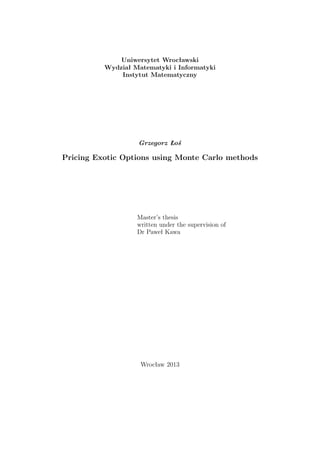
We have eight types of barrier options, as each of them is call or put, up or down, in or out.
They are all defined in a similar manner. The best way to get a grip on the barrier options
is possibly through a graphical example. Figure 2.1 discusses payoffs from an up-and-out call
option in three different scenarios.
Another modification of the vanilla options are the Asian options. Their payoff depends
on an average price of the asset during options lifetime.
Definition 2.10. Payoffs of Asian call and put options on asset S(i) with exercise date T and
strike price E, are given by
Ccall
asian = ( ¯S
(i)
T − E)+,
Cput
asian = (E − ¯S
(i)
T )+,
where
¯S
(i)
T =
1
K
K
j=0
S
(i)
j·T/K,
for some K.
So far we presented only options on one asset. Multi-asset options are also in usage, for
example basket options are options on the value η · S. Vector η describes quantity of shares
of the assets contained in a basket. The basket call option gives us right to buy whole set of
assets for the specified price, and the basket put allows us to sell it.
Definition 2.11. Payoffs of basket call and put options on basket η with exercise date T and
strike price E, are given by
Ccall
η = (η · ST − E)+,
Cput
η = (E − η · ST )+,
28. 28 2. Basics of option pricing
70
80
90
100
110
120
130
140
0.0 0.1 0.2 0.3 0.4 0.5 0.6 0.7 0.8 0.9 1.0
time
assetprice
Figure 2.1: Consider an up-and-out call option with strike 100, barrier 130, expiring at time 1. In the
red scenario the option is in-the-money at the maturity, however, in the past the barrier was crossed,
thus payoff is 0. In the blue scenario stock price ends about the level 113, the barrier was not reached,
hence the payoff equals 13. In case of the green scenario the payoff is 0, as it would be for vanilla option,
because the option ended out-of-the-money.
2.2.2 Motivation for the option usage
Why do we need derivatives in the first place? The well known anecdote claims that
the first man who used derivatives was Tales of Miletus. His skills allowed him to predict that
the olive harvest next year will be extraordinarily large. In the winter, when nobody needed
olive presses, he reserved them for summer. During the season demand for the olive presses
increased and Tales rented them for a good price. After all, it turned out that he earned much
more then paid for the reservation. From this story appears the first reason to use options: they
give opportunity to make money on accurate predictions.
Second, and probably more important reason of option usage, is possibility to hedge against
inconvenient scenarios. Consider a producer making his articles from some raw material. The
cost of his production depends on the price of this material. If it goes too high, then the factory
may become unprofitable. By buying the options, the producer may ensure that the cost of
the production will not exceed above known level. If the price of the raw material stays low,
then the options expire worthless, but the producer stays content, because the production is not
endangered. If asset price peaks, he can exercise the options. Either way he wins.
What is the purpose of exotic options? Altering the rules of “typical” payoffs may be
caused by many reasons. The seller of a call option puts himself into a risk, induced by the
fact, that his maximum possible loss is unbounded. Thus, he may be interested in entering only
contracts with up-and-out barrier, which prevents too large payoffs. The buyer of the call option
may want to hedge himself against high prices. He may purchase cheaper version of the option,
29. 2.3. Black-Scholes model 29
with down-and-out barrier – maybe if the asset price is low, he does not need any extra hedge.
Asian options may be a good choice for risk-averse investors, because they are less sensitive to
changes in the underlying price, especially in the time close to the maturity.
Both described stories show that derivatives idea arises in a natural way. In both stories
there was an exchange of the money for some goods. In the real live, however, situation is not
always that clear. Sometimes, even if the investor exercise his option on some commodity, there
is no real transaction performed, only the difference between prices is paid off. It may seem that
the derivatives are artificial tools, created by people living only in the theoretical, mathematical
models. Some exotic options may be really complicated and at the first glance no one can tell
what was the motivation of entering such contract. However, it is worth to remember, that
many of the derivative contracts are designed by investors, economist or producers, and they
correspond to their real needs. Mathematical models lend a hand in pricing such contracts.
2.3 Black-Scholes model
So far we discussed a very general market model. In order to obtain some specific results, we
have to make several more assumptions. In this section we recall famous Black-Scholes model,
leading to a straightforward formula for the price of the European options.
2.3.1 One-asset model
At first we discuss a case when d = 1, i.e. the model has only one risky asset and a bond. For
convenience we write S instead of S(1), and B instead of S(0). We use this convention every
time when considering a market with one risky asset.
The assumptions are following:
BS1. The market does not admit arbitrage opportunities.
BS2. The stock price of the underlying follows a geometric Brownian motion. More-
over drift µ and volatility σ are constant in time. Thus, SDE of the option price is described
by equation
dSt = µStdt + σStdWt. (2.4)
BS3. There exists constant risk-free interest rate r. In the other words, dynamics of B
is given by
dBt = rBtdt.
Investors may both, borrow and lend, any amount of money at rate r.
BS4. It is possible to buy and sell any amount of stock. It means that investors can even
trade fractional numbers of stock, and sell short unbounded quantity of shares.
BS5. All transactions do not incur any additional costs.
BS6. The underlying does not pay a dividend.
30. 30 2. Basics of option pricing
BS7. We have to make one additional assumption on the options value. Many authors forget to
mention it, although it is required for Itˆo’s lemma. Let F be the process of the option’s
price1. For some smooth function ϕ the price process has the form:
Ft = ϕ(St, t). (2.5)
This assumption looks entirely natural, but it cannot be concluded from what we discussed
so far. It must be taken as an axiom.
Instead of (2.5) we write Ft = F(St, t). Then F has an ambiguous meaning – left F denotes
the price process and the right one is some function. However, as in many other literature, we
identify them, since it does not lead to misunderstanding.
Suppose that we are constructing a portfolio consisting of a short position in one option
and a long position in ∆ shares. Let Π be the value process of the portfolio. Equation of the
portfolio is given by
Π = ∆S − F (2.6)
We analyse how much the portfolio changes in a short period of time. We have
dΠ = ∆dS − dF
Note that we do not have to differentiate ∆, because it is constant in an infinitesimal increment
of time. To handle dF we use Itˆo’s lemma. Thus
dΠ = ∆dS −
∂F
∂S
dS −
∂F
∂t
dt −
1
2
σ2
S2 ∂2F
∂S2
dt
The risk in an increment of the portfolio’s value is caused by changes of the stock price. By
choosing
∆ =
∂F
∂S
(2.7)
we get rid off the uncertainty. Now we have
dΠ = −(
∂F
∂t
+
1
2
σ2
S2 ∂2F
∂S2
)dt. (2.8)
The increment of Π does not depend on any risky asset, hence no-arbitrage assumption induces
dΠ = rΠdt.
After substituting (2.6), (2.7) and (2.8) into above equation, we obtain
−(
∂F
∂t
+
1
2
σ2
S2 ∂2F
∂S2
)dt = r(
∂F
∂S
S − F)dt,
which after simple calculation gives
∂F
∂t
+
1
2
σ2
S2 ∂2F
∂S2
+ r
∂F
∂S
S − rF = 0. (2.9)
1
Ft is the value of the option quoted at time t (not discounted to time 0). The discounted price process is in
this thesis denoted by letter V .
31. 2.3. Black-Scholes model 31
Formula (2.9) is known as the Black-Scholes equation. Note that so far we did not say
anything about the final condition of (2.9), i.e. about the payoff off the option, thus this is
a general equation. For European options it has straightforward solution, known as Black-
Scholes formula.
Proposition 2.2. Prices of the European call and put options with time to the expiration T,
strike price E and the underlying dynamics given by (2.4) are given by the following equations:
Ft
call
= StΦ d1(t) − e−r(T−t)
EΦ d2(t) ,
Ft
put
= −StΦ −d1(t) + e−r(T−t)
EΦ −d2(t) ,
where
d1(t) =
ln St
E + r + σ2
2 (T − t)
σ
√
T − t
d2(t) =
ln St
E + r − σ2
2 (T − t)
σ
√
T − t
= d1(t) − σ
√
T − t,
Φ is the distribution function of the standard normal distribution.
We prove this proposition at the end of the section 2.5, using the risk-neutral measure.
2.3.2 Multi-asset model.
All assumptions for a one-asset model carry over almost instantly to a multi-asset model with
just a little edition:
BS2. Stock prices of all risky assets follow a geometric Brownian motion. Each risky
asset S(i) has constant drift µi and volatility σi. In symbolic form:
dS
(i)
t = µS
(i)
t dt + σS
(i)
t dW
(i)
t (i = 1, 2, . . . , d). (2.10)
BS3. The dynamics of S(0) is given by
dS
(0)
t = rS
(0)
t dt.
The movements of the asset prices are usually not independent.
Definition 2.12. We say that the correlation between two risky assets S(i) and S(j) equals ij
if and only if Corr(W(i), W(j)) = ij.
In the other words by the correlation of two assets we understand the correlation between
corresponding Wiener processes, appearing in their dynamics. A matrix of the correlation
between all risky processes is denoted by Σ,
Σ =
11 12 · · · 1d
21 22 · · · 2d
...
...
...
...
d1 d2 · · · dd
.
The assumptions described in this section hold true to the rest of the thesis.
32. 32 2. Basics of option pricing
2.4 Model calibration
By looking at the previous section we can specify a set of values by which the model is param-
eterized:
• drifts µ1, µ2, . . . , µd,
• volatilities σ1, σ2, . . . , σd,
• correlation Σ,
• riskless interest rate r.
While calibrating a model it is convenient to assume that today is time 0. We are interested
in modelling asset prices in the future, up to time T. It is natural to use negative t to denote
times in the past. For example S
(i)
−0.5 means the price of the ith asset half of a year ago. Hence
for t > 0, St is random vector, which we are about to model, and for t ≤ 0, St is a vector with
historical prices, which may be obtained from the stock archives.
Since asset prices follow (2.10) and its solution is given by (1.4), thus for all i
S
(i)
tn+1
= S
(i)
tn
exp (µi −
1
2
σ2
i )∆t + σi
√
∆tZi ,
where ∆t = tn+1 − tn, Z is a random vector with correlation matrix Σ = ij
d
i,j=1
, and for each
Zi, Zi ∼ N(0, 1). Let
L
(i)
n+1 = ln
S
(i)
tn+1
S
(i)
tn
.
It is clear that L
(i)
n+1 ∼ N (µi − 1
2σ2
i )∆t, σ2
i ∆t
The key to the calibration is an assumption that in the past, price processes followed (2.10)
as well. Let T denote how old is the oldest price observation, and N be such that N · ∆t = T.
Furthermore let tk = −(N − k)∆t (k = 0, 1, . . . , N). Values tk are times in which we take
historical prices, from t0 = −T, to tN = 0, which is today. Let us focus on the ith asset. We
have N + 1 historical prices:
S
(i)
t0
, S
(i)
t1
, . . . , S
(i)
tN
,
from which we obtain a vector
L
(i)
1 , L
(i)
2 , . . . , L
(i)
N
with N samples from the distribution N (µi − 1
2σ2
i )∆t, σ2
i ∆t .
In practice, usually ∆t = 1/252, because there are about 252 working days in a year. How-
ever, it is debatable how long should be T.
Finally, we present how to obtain values of model parameters.
33. 2.4. Model calibration 33
Drifts and volatilities. Let L(i) ∼ N (µi − 1
2σ2
i )∆t, σ2
i ∆t . It means that
E L(i)
= (µi −
1
2
σ2
i )∆t,
Var L(i)
= σ2
i ∆t.
Hence
µi =
2E L(i) + Var L(i)
2∆t
,
σ2
i =
Var L(i)
∆t
.
Now we can use the sample vector to estimate expectation and variance. Let
αi =
1
N
N
k=1
L
(i)
k
βi =
1
N − 1
N
k=1
(L
(i)
k − αi)2
Values αi and βi are unbiased estimators of expectation and variance respectively. Thus we
assign
µi =
2αi + βi
2∆t
,
σ2
i =
βi
∆t
.
Remark 2.2. Calculating drifts is in many applications redundant. Note that there is no drift
term in Black-Scholes formula nor equation. As it is shown in section 2.5 also the dynamics in
the martingale measure does not depend on the drift.
Correlation. At first recall that Corr(aX+b, cY +d) = Corr(X, Y ). Thus finding a correlation
between Zi and Zj is equivalent to finding correlation between L(i) and L(j). We can do it using
Pearson’s estimator:
i,j =
1
N − 1
N
k=1
(L
(i)
k − αi)(L
(j)
k − αj)
βiβj
Riskless interest rate. In order to calculate the interest rate it is necessary to choose a bond
whose maturity is close to the expiry of the valued option. The interest rate implied by that
bond reflects well the real interest rate in the concerned time.
It is clear that
C = Ne−rT
,
34. 34 2. Basics of option pricing
where C is price of the bond, N is its nominal value, r is the interest rate implied by the bond,
and T is the maturity time. By simple transformation
r =
ln(N
C )
T
.
2.5 Pricing general contingent claims
Black-Scholes formula allows us to price only European vanilla options. In this section we present
a general method for pricing European contingent claims.
2.5.1 Risk neutral pricing
Definition 2.13. The discounted value of the contingent claim C is given by
H =
C
S
(0)
T
.
Random variable H is called a discounted claim.
Values C and H correspond to the payoff of an instrument. We need notation to talk about
its price also before the expiration.
Definition 2.14. The (discounted) price process of the contingent claim is denoted by Vt.
The next theorem is the key to defining prices of contingent claims. But first we define a
class of claims for which valuation is pretty straightforward.
Definition 2.15. A contingent claim is called attainable if there exists a self-financing trading
strategy ¯ξ whose portfolio coincides with C at the expiration, i.e.
C = ¯ξ · ¯ST .
The trading strategy ¯ξ is then called the replicating strategy for C.
Theorem 2.3. For every attainable discounted claim H and for every equivalent martingale
measure P∗
E∗
[H] < ∞.
Moreover, for every replicating strategy ¯ξ its value process satisfies
V ξ
t = E∗
[H|Ft] P-a.s., 0 ≤ t ≤ T. (2.11)
Proof of this theorem reader may find in [2] (Theorem 5.26).
Since there is no ¯ξ in term E∗[H|Ft], so value V ξ
t does not depend on choice of ¯ξ. Note also
that
E∗
[H|Ft] = E∗
[¯ξ · ¯XT |Ft] = ¯ξ · ¯Xt
35. 2.5. Pricing general contingent claims 35
Thus, value E∗[H|Ft] does not depend on the choice of P∗ . Since attainable discounted claim
H and its replicating strategy ¯ξ have the same payoff at time T, thus no-arbitrage assumption
induces
Vt = V ξ
t , 0 ≤ t ≤ T.
Thus in particular it implies
Corollary 2.4 (Risk neutral valuation formula). Let H be a discounted attainable contin-
gent claim and V be its price process. Then
V0 = E∗
[H]. (2.12)
This equation tells us that the value of the option is an expectation of its discounted
payoff under the risk-neutral measure.
The above theorem suggests how price processes should look in general.
Definition 2.16. The (discounted) price process of the discounted claim H is given by
Vt = E∗
[H|Ft].
Such V is a P∗ -martingale.
For general claims process V depends on the choice of an equivalent martingale measure.
However, it may be proven that the market model consisting of the discounted assets
(X(0)
, X(1)
, . . . , X(d)
, V )
is arbitrage-free, regardless of the choice of P∗ . In that sense every possible price process V is
equally good.
2.5.2 Change of the measure
The martingale measure allows us to write the option’s value if a form of a concise formula, but
so far we did not tell how to find it. It turns out that we do not really need the martingale
measure itself. The only matter is how the asset’s price process can be expressed under the risk
neutral measure.
In the literature there are many formulations of the theory which is presented here. However,
instead of referring to any other authors, we will prove some facts which exactly match our needs.
Lemma 2.5. Suppose that S is a d-dimensional stochastic process, where each S(i) follows the
geometric Brownian motion, that is
dS(i)
= µiS(i)
dt + σiS(i)
d ¯W(i)
, (i = 1, 2, . . . , d) (2.13)
where each ¯W(i) is a Brownian motion under measure P and Corr( ¯W(i), ¯W(j)) = ρij. For every
vector (ν1, ν2, . . . , νd) there exists an equivalent probability measure Q, such that the equation
(2.13) may be rewritten in the form
dS(i)
= νiS(i)
dt + σiS(i)
dW(i)
, (i = 1, 2, . . . , d) (2.14)
where each W(i) is a Brownian motion under the equivalent measure Q and
CorrQ
(W(i), W(j)) = ρij.
36. 36 2. Basics of option pricing
Proof. Let Σ = (ρij)d
i,j=1 be a correlation matrix. Cholesky’s algorithm allows us to decompose
Σ to the form
Σ = LLT
,
where L is lower triangular matrix. Hence, ¯W may be written in the form
¯W = L ¯V ,
where ¯V is a standard d-dimensional Wiener process under measure P . Let us apply Theorem
1.3 (Girsanov theorem) with ϕ := θ = (θ1, θ2, . . . , θd) , where all θi are some constants. It implies
that
Vt = ¯Vt − tθ
is a d-dimensional standard Wiener process under an equivalent measure Q, which is defined as
dQ
dP
= exp
d
i=1
θi
¯W
(i)
T −
T
2
||θ||2
.
Let W := LV . Thus
dS(i)
= µiS(i)
dt + σiS(i)
d ¯W(i)
= µiS(i)
dt + σiS(i)
d
i
k=1
lik
¯V (k)
= µiS(i)
dt + σiS(i)
d
i
k=1
likθkt + likV (k)
= µi + σi
i
k=1
likθk S(i)
dt + σiS(i)
d
i
k=1
likV (k)
= µi + σi
i
k=1
likθk S(i)
dt + σiS(i)
dW(i)
.
By substituting
θ1 :=
ν1 − µ1
σ1l11
θi :=
νi − µi − σi
i−1
k=1
likθk
σilii
(i = 2, 3, . . . , d)
we get the thesis.
The above lemma allows us to describe the vector of price processes in terms of some equiv-
alent measures, however we need a very particular measure – the martingale measure.
37. 2.5. Pricing general contingent claims 37
Proposition 2.6. Under the real measure P the risky assets follow a geometric Brownian mo-
tion, as in equation (2.13). There exists an equivalent martingale measure P∗ , such that the
dynamics has the form
dS(i)
= rS(i)
dt + σiS(i)
dW(i)
. (2.15)
Proof. Lemma 2.5 states that there exists an equivalent measure P∗ under which price processes
are described by equation (2.15). We show that it is martingale measure. From (1.4)
Xt = e−rt
St = S0e−1
2
σ2t+σWt
.
Let 0 ≤ s ≤ t ≤ T. We have
E∗
[Xt|Fs] = E∗
[S0e−1
2
σ2t+σWt
|Fs]
= S0e−1
2
σ2t
· E∗
[eσWs
eσ(Wt−Ws)
|Fs]
= S0e−1
2
σ2t+σWs
· E∗
[eσ(Wt−Ws)
]
= S0e−1
2
σ2t+σWs
e
1
2
σ2(t−s)
= S0e−1
2
σ2s+σWs
= Xs.
Hence P∗ is an equivalent martingale measure.
Propositions 2.6 and 1.2 have crucial meaning in our applications. They allow us to generate
trajectories of the asset prices under the risk-neutral measure, which is essential in the Monte
Carlo pricing. We show one more application of the risk-neutral pricing – it can be used to
derive Black-Scholes formula.
(Proof of Proposition 2.2). From Proposition 1.2
ST = St exp (r −
1
2
σ2
)(T − t) + σWT−t = SteZ
,
where Z ∼ N (r − 1
2σ2)(T − t), (T − t)σ2 in the measure P∗ . Let fZ be the density of Z and
St = s, thus
Ft
call
= e−r(T−t)
E∗
[(ST − E)+|Ft]
== e−r(T−t)
E∗
[(ST − E)+|St]
= e−r(T−t)
E∗
(seZ
− E)+
== e−r(T−t)
E∗
(seZ
− E) · 1 Z ≥ ln E
s
= e−r(T−t)
∞
ln(E/s)
(sez
− E)fZ(z)dz
= s
∞
ln(E/s)
e−r(T−t)
ez
fZ(z)dz − e−r(T−t)
E
∞
ln(E/s)
fZ(z)dz = ( )
38. 38 2. Basics of option pricing
Simple calculation gives
∞
ln(E/s)
e−r(T−t)
ez
fZ(z)dz = Φ d1(t) ,
∞
ln(E/s)
fZ(z)dz = Φ d2(t) ,
hence
( ) = StΦ d1(t) − e−r(T−t)
EΦ d2(t) .
Derivation of the formula for put’s price is analogous.
39. III
Pricing European options using
Monte Carlo method
The Black-Scholes theory gives us compact formula for pricing European vanilla options. Such
options gained popularity and are traded in many world markets. However, over the counter
(ab. OTC) investors may trade much more complicated instruments, whose value cannot be
derived analytically. Thus, other methods must be used. The most popular are finite difference,
binomial trees and Monte Carlo. In this thesis we present the last one.
3.1 Vanilla options
In order to use the Monte Carlo method in the option pricing, we need to involve the theory
presented in the section 2.5. First we focus on the case, when the only instruments traded in
the market are B = S(0) – a riskless bank account, and a risky asset S = S(1).
As in previous chapter, V0 is the option’s price and H is the discounted payoff. From
Corollary 2.4 we have
V0 = E∗
[H]. (3.1)
By comparison with (1.5), we see that equation (3.1) is exactly what we need for simulations.
To calculate options price we have to replicate its payoff many times and take the mean. Note,
however, that expectation is taken under the risk-neutral measure. Hence, also the asset price
must be generated under the risk-neutral measure. Corollary 2.6 describes its dynamics:
dS = rSdt + σSdW.
Proposition 1.2 gives the solution to above SDE:
St = S0 exp (r −
1
2
σ2
)t + σWt . (3.2)
In case of vanilla options only the value at the end of the trajectory is important, i.e. at maturity
time T. Thus, we need
ST = S0 exp (r −
1
2
σ2
)T + σWT , (3.3)
39
40. 40 3. Pricing European options using Monte Carlo method
where, from properties of the Wiener process, WT ∼ N(0, T). The value of ST depends on WT ,
hence it is justified to treat ST as a function of WT and write ST = ST (WT ).
Let H = g(ST ) and E be the strike price. For instance, if H is a call option
g(x) = e−rT (x − E)+, and if H is a put g(x) = e−rT (E − x)+, but in fact H might be any
claim whose payoff depends only on ST . Equation (3.3) tells us how to generate the asset price;
by applying function g we generate the payoff. Since ST is also a function of some Z ∼ N(0, T),
thus actually H = g(ST (Z)) =: f(Z), for f = g ◦ ST . By Zi, i = 1, 2, ..., we denote replications
of Z. The crude Monte Carlo estimator has the form:
ˆHCMC
2n =
1
2n
2n
i=1
f(Zi). (3.4)
We also use antithetic variates, where an antithetic variable to f(Zi) is f(−Zi).
ˆHAV
n =
1
n
n
i=1
f(Zi) + f(−Zi)
2
. (3.5)
To use the control variates method, recall that erT S0 = E∗[ST ]. It implies that we can take ST
as a control variate, hence
ˆHCV
n =
1
n
n
i=1
f(Zi) + c(ST (Zi) − erT
S0) , (3.6)
where c is a value calculated as in equation (1.14).
To get a grip on using above estimators in practice, we present how exactly looks pricing
call options using the control variates method. It is shown in Algorithm 3.1. Argument of the
algorithm is n – number of simulations. Values calculated in lines 12-14 are price of the option,
variance and standard error of the estimation.
An implementation of an option pricer based on estimators (3.4)-(3.6) allows us to compare
these methods. In sections 3.1 and 3.2 we always assume following parameters:
S = 100
σ = 0.20
r = 0.05
T = 1 (options expire after one year).
(3.7)
Example 3.1. First consider a call option with strike 90. The Black-Scholes value of the
option is 16.70. Results of the Monte Carlo pricing are shown in Table 3.1 and Figure 3.1.
It is clear, that in this case CV method proved itself the best. It is caused by the fact, that
in most simulations option expires in the money. In consequence the payoff is highly correlated
with the asset price at the end of the path. ♦
41. 3.1. Vanilla options 41
Algorithm 3.1 Valuation of a call option using CV method.
1: function PriceCallCV(n, S0, σ, r, T, E )
2: S, H, Y ← arrays with indices from 1 to n.
3: for i = 1 to n do
4: Z ← generate standard normal
5: S[i] ← S0 · exp{(r − 1
2σ2) · T + σ · Z}
6: H[i] ← max(S − E, 0) · exp{−rT}
7: end for
8: c ← −Cov(H, S)/Var(S)
9: for i = 1 to n do
10: Y [i] ← H[i] + c · S[i] − S0 · exp{rT}
11: end for
12: price ← mean(Y )
13: var ← var(Z)
14: se ← var/n
15: return (price, var, se)
16: end function
Table 3.1: Results of pricing call@90. Black-Scholes price is 16.70.
CMC AV CV
log10(n) ˆHCMC
2n s.e. ˆHAV
n s.e. ˆHCV
n s.e.
3 17.09 0.393 16.67 0.185 16.74 0.127
4 16.98 0.123 16.66 0.061 16.67 0.041
5 16.71 0.039 16.67 0.019 16.70 0.013
6 16.69 0.012 16.70 0.006 16.70 0.004
16.50
16.70
16.90
17.10
CMC AV CV
method
Estimatedvalue
method
AV
CMC
CV
16.20
16.40
16.60
16.80
0 25000 50000 75000 100000
replicated pairs
estimatedvalue
method
av
cmc
cv
Figure 3.1: The accuracy of pricing call@90. Box plot on the left was created by running estimation 100
times for each method, each estimation used 10000 replicated pairs. The chart on the right shows speed
of the convergence, i.e. how the estimation changes as the number of performed replications increases.
The horizontal line is the options value calculated form Black-Scholes formula.
42. 42 3. Pricing European options using Monte Carlo method
Example 3.2. Let us consider now a call with higher strike, 130, whose Black-Scholes price
equals 1.64. Look at the Table 3.2 and Figure 3.2.
This time the asset price usually ended above the options strike, what means that in most
simulations payoff was 0. Thus, correlation between payoff and assets final price is low, and in
consequence CV did not bring a significant improvement. ♦
Table 3.2: Results of pricing call@130. Black-Scholes price is 1.64.
CMC AV CV
log10(n) ˆHCMC
2n s.e. ˆHAV
n s.e. ˆHCV
n s.e.
3 1.67 0.135 1.56 0.126 1.67 0.147
4 1.61 0.043 1.60 0.041 1.60 0.046
5 1.63 0.014 1.64 0.013 1.64 0.015
6 1.64 0.004 1.64 0.004 1.64 0.005
1.60
1.70
CMC AV CV
method
Estimatedvalue
method
AV
CMC
CV 1.60
1.70
0 25000 50000 75000 100000
replicated pairs
estimatedvalue
method
av
cmc
cv
Figure 3.2: The accuracy of pricing call@130. Plots were created in the similar manner as in Figure 3.1.
Remark 3.1. Box plot from Figure 3.2 shows that CMC estimator has smaller dispersion than
AV and CV. That is because we compare ˆHCMC
2n (index is 2n) with ˆHAV
n and ˆHCV
n . We do so,
because then the number of used random variables is the same in each estimator. However,
generating an antithetic variate or a control variate is often instantaneous. Hence, in many
cases calculating ˆHCMC
2n may take almost twice as much time. If in time t we can compute ˆHCMC
a ,
ˆHAV
b and ˆHCV
c , then ˆHCMC
a always1 has greater variance than ˆHAV
b and ˆHCV
c .
1
Of course we assume that antithetic variate is really antithetic, i.e. it is negatively correlated with the base
variate, and control variate is not independent from the base variate.
43. 3.2. Path-dependent instruments 43
3.2 Path-dependent instruments
To price vanilla options it was sufficient to generate the asset price only at the maturity. However,
there are contingent claims whose payoff depends on the entire history, for example barrier
options or Asian options. Of course, we cannot generate the entire trajectory, since it has
continuum points. Thus, values of the asset must be generated in a finite number K of points.
To approximate a continuous model we have to take sufficiently large K.
It follows from equation (3.2) that
St+∆t = St exp (r −
1
2
σ2
)∆t + σ
√
∆tZ , (3.8)
where Z is standard normal. The above formula allows us to generate asset’s prices in specified
points step by step.
Figure 3.3 shows a thousand of trajectories simulated accordingly to equation (3.8). Note
that the mean of the asset price at the final time is slightly above S0 = 100. It corresponds to
the fact that E∗[ST ] = erT S0, which for parameters of the simulations equals 100·e0.05 ≈ 105.13.
50
60
70
80
90
100
110
120
130
140
150
160
170
180
190
0.0 0.1 0.2 0.3 0.4 0.5 0.6 0.7 0.8 0.9 1.0
time
assetprice
Quartile.3rd
Mean
Median
Quartile.1st
Figure 3.3: A thousand of simulated trajectories of the asset price, under parameters T = 1, σ = 0.2,
r = 0.05, S0 = 100. Each path was generated in K = 50 points. The darker is the area the greater is the
concentration of trajectories.
In theory, the value of the discounted claim now has the form H = g(S), for some g,
i.e. H is a function of the whole process S. As mentioned before, in order to make H com-
putable, we are forced to treat H as a function of S in limited number of points, that is
H = g S0, S∆t, ..., ST , T = K · ∆t.
44. 44 3. Pricing European options using Monte Carlo method
Further in this chapter we use the following notation. Path replications are denoted by
Si (i = 1, 2, ...), and value Si,t means what was the asset price at time t, on i-th simulated path.
The CMC estimator is analogous to (3.4)
ˆHCMC
n =
1
n
n
i=1
g Si,0, Si,∆t, ..., Si,T
For example for Asian call option
ˆHCMC
n =
1
n
n
i=1
1
K
K
j=0
Si,j∆t − E
+
and for a put option with down-and-out barrier B
ˆHCMC
n =
1
n
n
i=1
(E − Si,T )+ ·
K
j=0
1 Si,j∆t ≥ B
.
Adjusting above estimators to use control variates does not bring any difficulties. The asset price
at the end of the path may still be the control variate, however, for many contingent claims a
better control variate is the payoff from a similar vanilla option. For instance for Asian put
option
ˆHCV
n = ˆHCMC
n +
c
n
n
i=1
(E − Si,T )+ − E∗
(E − ST )+ ,
where c is calculated as in (1.14) and value E∗(E − ST )+ is known from the Black-Scholes
formula.
In previous section while using AV method, we generated negatively correlated variables
representing the asset price at the option’s expiry. Since now, payoff depends on the whole
process, thus we have to generate the antithetic trajectories. Algorithm 3.2 presents a proper
procedure. Figure 3.4 gives an idea how antithetic paths look like. We omit exact formulas
for ˆHAV
n , because they are becoming lengthy and overly complicated. Analysing an example
application of AV method should be sufficient to understand how it works in general. To this
end, we present procedure of pricing Asian call options (Algorithm 3.3).
In a similar manner we can value any path-dependent options. For instance we present
results of pricing some barrier options. In this section we still set market parameters as in (3.7),
moreover we take
K = 50,
it may be regarded as checking once a week if the barrier was hit. As a control variate we used
the payoff from a vanilla put with strike equal to the spot price (i.e. 100).
45. 3.2. Path-dependent instruments 45
90
100
110
120
130
0.00 0.25 0.50 0.75 1.00
time
assetprice
variable
Positive
Negative
Figure 3.4: One pair of antithetic trajectories generated by an implementation of Algorithm 3.2.
Algorithm 3.2 Generating antithetic trajectories.
1: function Trajectory(S0, σ, r, T, K)
2: pos, neg ← arrays with indices from 0 to K
3: pos[0] ← neg[0] ← S0
4: dt ← T/K
5: for i = 1 to K do
6: Z ← generate standard normal
7: pos[i] ← pos[i − 1] · exp (r − 1
2σ2)dt + σ
√
dtZ
8: neg[i] ← neg[i − 1] · exp (r − 1
2σ2)dt − σ
√
dtZ
9: end for
10: return (pos, neg)
11: end function
Algorithm 3.3 Pricing Asian call options
1: function PriceAsianCallAV(n, S0, σ, r, T, E, K)
2: sum ← sum sq ← 0
3: for i = 1 to n do
4: (pos,neg) ← Trajectory(S0, σ, r, T, K)
5: Hpos ← max(mean(pos)−E, 0) · exp{−rT}
6: Hneg ← max(mean(neg)−E, 0) · exp{−rT}
7: H ← 1
2 · (Hpos + Hneg)
8: sum ← sum + H
9: sum sq ← sum sq + H2
10: end for
11: var ← (sum sq − sum · sum/n)/(n − 1)
12: se ← var/n
13: price ← sum/n
14: return (price, var, se)
15: end function
46. 46 3. Pricing European options using Monte Carlo method
Example 3.3. Suppose that S is an exchange rate between some currencies. Consider an
exporter whose production becomes unprofitable when exchange rate becomes too low. He would
like to be hedged for pessimistic scenarios, thus he is interested in purchasing put options with
strike 100, whose price from the Black-Scholes formula is 5.57. In order to save some capital he
prefers cheaper barrier options rather than vanilla options. He may think the following: “If the
exchange rate at some point will be very high, then the profit made at that time will cover any
eventual losses when the rate sinks down”. Thus he may decide to buy put options with strike
100 and with up-and-out barrier 115.
Monte Carlo methods allow us to price such an instrument, and the results are gathered in
Table 3.3 and Figure 3.5. ♦
Table 3.3: Results of pricing put@100 with an up-and-out barrier 115. Black-Scholes price of the option
without barrier equals 5.57.
CMC AV CV
log10(n) ˆHCMC
2n s.e. ˆHAV
n s.e. ˆHCV
n s.e.
3 5.10 0.189 5.13 0.150 5.20 0.072
4 5.14 0.060 5.15 0.049 5.15 0.023
5 5.20 0.019 5.17 0.015 5.18 0.007
6 5.18 0.006 5.17 0.005 5.18 0.002
5.00
5.10
5.20
5.30
CMC AV CV
method
Estimatedvalue
method
AV
CMC
CV
5.20
5.30
5.40
5.50
0 25000 50000 75000 100000
replicated pairs
estimatedvalue
method
av
cmc
cv
Figure 3.5: The accuracy of pricing put@100 with an up-and-in barrier 115. Plots were created in the
similar manner as in Figure 3.1.
Example 3.4. On the other hand, the exporter from the previous example may think: “My
losses are not too severe, until the exchange rate sinks down extremely low. In this case I would
like to retrieve my losses at the option’s expiration date.”. Hence, he may be interested in put
options with strike 100 and with down-and-in barrier 70. Table 3.4 and Figure 3.6 present results
of pricing such instrument with Monte Carlo methods. ♦
As previously, CV seems to be the best method when payoffs from vanilla option and barrier
options are highly correlated. It is the case during the valuation of put@100 with up-and-out
barrier 115. The option expires in the money when asset prices are low, while reaching the
47. 3.3. Multi-asset instruments 47
Table 3.4: Results of pricing put@100 with down-and-in barrier 70. Black-Scholes price of the option
without barrier equals 5.57.
CMC AV CV
log10(n) ˆHCMC
2n s.e. ˆHAV
n s.e. ˆHCV
n s.e.
3 1.33 0.138 1.38 0.135 1.37 0.152
4 1.29 0.043 1.31 0.043 1.31 0.049
5 1.38 0.014 1.36 0.014 1.36 0.016
6 1.35 0.004 1.35 0.004 1.36 0.004
1.20
1.30
1.40
CMC AV CV
method
Estimatedvalue
method
AV
CMC
CV
1.20
1.40
1.60
0 25000 50000 75000 100000
replicated pairs
estimatedvalue
method
av
cmc
cv
Figure 3.6: The accuracy of pricing put@100 with a down-and-in barrier 70. Plots were created in the
similar manner as in Figure 3.1.
barrier happens when prices are high. Hence, in most cases if the option ended in the money,
then the barrier was not hit, and if the barrier was hit, then the option would expire worthless
anyway. Thus, the payoff of barrier and vanilla options are highly correlated.
In the case of put@100 with down-and-in barrier 70, the barrier is set very low; hitting it
happens seldom, thus often the option expires worthless even if an analogous vanilla option ends
in the money. In consequence the correlation between payoffs of the barrier and vanilla options
becomes low, and in this case AV method gives slightly better accuracy.
At the end of this section, it is worth to mention, that there exist analytical formulas for
prices of European barrier options, see [6], chapter 23.
3.3 Multi-asset instruments
The valuation of derivatives whose payoff depends on many assets does not differ much from one
dimensional case. We only have to remember to include correlations between the assets. Let
Σ = ( ij)d
i,j=1
be the matrix describing correlation between risky assets (recall that by that we understand the
correlation between Wiener processes appearing in assets dynamics). Equation (3.8) holds for
48. 48 3. Pricing European options using Monte Carlo method
every asset, i.e.
S
(i)
t+∆t = S
(i)
t exp (r −
1
2
σ2
i )∆t + σi
√
∆tZi (i = 1, 2, . . . , d), (3.9)
where each Zi is standard normal. However, we have to take into account correlation between
variables Zi. To be precise Z ∼ N(0, Σ).
Equation (3.9) is the key to generating multi-asset scenarios. Its usage is shown in Algorithm
3.4, which creates two antithetic scenarios of market evolution. Figure 3.7 illustrates trajectories
of prices of correlated assets.
Algorithm 3.4 Generating multi-asset trajectories.
1: function MultiTrajectory(S0, σ, r, Σ, T, K)
S0 and σ are now arrays, for example σ[3] is the volatility of the third asset
2: S ← two dimensional array S[i,k] is the price of i-th asset at k-th time point
3: S ← two dimensional array antithetic scenario
4: L ← Cholesky decomposition of Σ Σ = LL
5: for i = 1 to d do
6: S[i, 0] ← S0[i]
7: S [i, 0] ← S0[i]
8: end for
9: dt ← T/K
10: for k = 1 to K do
11: Z ← array of d independent standard normal variates
12: Z ← LZ now Z is a sample from N(0, Σ) distribution
13: for i = 1 to d do
14: S[i, k] ← S[i, k − 1] · exp (r − 1
2σ[i]2)dt + σ[i]
√
dtZ[i]
15: S [i, k] ← S [i, k − 1] · exp (r − 1
2σ[i]2)dt − σ[i]
√
dtZ[i]
16: end for
17: end for
18: return (S, S )
19: end function
Remark 3.2. If the payoff depends only on the assets values at the end of the path, then there is
no need to generate whole trajectories. It is sufficient to generate asset prices only at the expiry,
using equations
S
(i)
T = S
(i)
0 exp (r −
1
2
σ2
i )T + σi
√
TZi (i = 1, 2, . . . , d),
where Z ∼ N(0, Σ). We do not have to write a new algorithm to do that, we can use function
MultiTrajectory with K = 1.
Since we have a method for scenario generation, valuation of the multi-asset options is
pretty straightforward. For example we write a procedure for pricing basket put options using
49. 3.3. Multi-asset instruments 49
40
60
80
100
0.00 0.25 0.50 0.75 1.00
time
assetsprices
Figure 3.7: Price trajectories of correlated assets. The correlation between red and green equals 0.8,
between red and blue -0.8, and between green and blue also -0.8.
AV method. The basket is described by an array η, where η[i] means how many units of i-th
asset are contained in a basket. In Algorithm 3.5 we called function MultiTrajectory with
K = 1, because payoff of the basket option does not depend on the history.
Algorithm 3.5 Pricing basket put option.
1: function PriceBasketPutAV(n, S0, σ, r, Σ, T, η, E)
2: sum ← sum sq ← 0
3: for j = 1 to n do
4: (S, S ) ← MultiTrajectory(S0, σ, r, Σ, T, 1)
5: H ← 1
2 exp{−rT}( BasketPutPayoff(S, η, E, 1) +
6: BasketPutPayoff(S , η, E, 1) )
7: end for
8: var ← (sum sq − sum · sum/n)/(n − 1)
9: se ← var/n
10: price ← sum/n
11: return (price, var, se)
12: end function
13: function BasketPutPayoff(S, η, E, K)
14: sum ← 0
15: for i = 1 to d do
16: sum ← sum + η[i] · S[i, K]
17: end for
18: return max(E − sum, 0)
19: end function
Modifications of options and their payoffs are only bounded by investors imagination, how-
ever, it should be clear how to modify Algorithm 3.5 to price options with any arbitrary payoff,
even path-dependent. This is the main advantage of Monte Carlo methods in option pricing –
flexibility, which cannot be provided by the finite difference or binomial trees.
50. 50 3. Pricing European options using Monte Carlo method
Example 3.5. We used the described technique to price a basket vanilla call option. We took
following parameters:
d = 3, S0 = (10, 50, 100)
r = 0.05, σ = (0.4, 0.2, 0.3),
Σ =
1 0.8 −0.8
0.8 1 −0.8
−0.8 −0.8 1
E = 90, η = (10, −2, 1), T = 1
(3.10)
Such contract at the expiration date gives its owner right to change 2 shares of the second asset
and amount of money E for 10 shares of the first asset and one of the third. The results are
gathered in Table 3.5 and Figure 3.8. In CV method value of the basket at the expiry was used
as the control variate. From section 2.5 we know its expectation: E∗[η ·ST ] = η ·S0. CV method
gave the most accurate prices. ♦
Table 3.5: Results of pricing the basket option described in equations (3.10).
CMC AV CV
log10(n) ˆHCMC
2n s.e. ˆHAV
n s.e. ˆHCV
n s.e.
3 18.91 0.507 19.90 0.444 19.85 0.241
4 19.66 0.165 19.84 0.143 19.73 0.077
5 19.65 0.052 19.68 0.045 19.70 0.024
6 19.72 0.017 19.70 0.014 19.70 0.008
19.50
19.75
20.00
20.25
CMC AV CV
method
Estimatedvalue
method
AV
CMC
CV
19.50
19.80
20.10
20.40
0 25000 50000 75000 100000
replicated pairs
estimatedvalue
method
av
cmc
cv
Figure 3.8: The accuracy of pricing basket option described in equations (3.10). Prices calculated using
AV and CMC methods look like they were converging to different values. It is caused by the fact, that
one price is underestimated and the second is overestimated. However, in both cases the distance to the
correct value 19.70 is not greater than two standard errors. It means that the above plot gives us no
reason to worry – for greater numbers of simulations green and red lines would “stick” to each other
almost surely.
51. IV
Pricing American options using
Least Squares Monte Carlo
In chapter IV we describe American-style derivatives. The difference between them and previ-
ously discussed European-style contracts is that the American feature allows the owner of the
derivative to exercise it in any time up to the expiration date. This additional attribute makes
the instrument much harder to analyse and more advanced theory is necessary to value and
hedge it. Due to the practical nature of this thesis we do not get deep into details. Nevertheless,
we provide mathematical tools necessary for pricing American contingent claims, advising the
reader to find proofs in the more specialized literature.
It turns out that the Monte Carlo method from previous chapter cannot be carried over di-
rectly to price American contracts. However, we describe a method invented by Francis Longstaff
and Eduardo Schwartz, called the Least Squares Monte Carlo. It introduces a clever trick, so
the simulations can still be involved.
4.1 American contingent claims
In opposite to European contingent claims, American contingent claims are not random vari-
ables, but processes.
Definition 4.1. An American contingent claim is a non-negative adapted process C =
(Ct)T
t=0 on the filtered probability space (Ω, F, (Ft)T
t=0, P ). From now on by a derivative of the
underlying assets ¯S we understand such American contingent claim C which is adapted also to
the filtration generated by ¯S (which in general may be smaller than F).
Value Ct may be interpreted as the payoff obtained from the claim if it is exercised at time t.
The definitions from section 2.2 carry over directly to their American counterparts, for example
American call and put options on the ith asset are defined as derivatives with the payoffs
Ccall
t = (S
(i)
t − E)+,
Cput
t = (E − S
(i)
t )+,
51
52. 52 4. Pricing American options using Least Squares Monte Carlo
where E is the strike price.
Remark 4.1. European contracts are in fact a particular case of American contracts. An Euro-
pean claim ˜C may be seen as an American claim C = (Ct)T
t=0 with payoff
Ct =
˜C, t = T
0, t < T.
As usually, it is convenient to quote payoff values in terms of time 0.
Definition 4.2. The discounted value of the American contingent claim C is a process H =
(Ht)T
t=0 given by
Ht =
Ct
S
(0)
t
.
The process H is called an American discounted claim.
4.1.1 Exercise strategies
The exercise time is entirely up to the buyer. He or she dynamically decides when to claim
the payoff, watching the market evolution. However, at the very beginning he or she may plan
under which conditions the option should be exercised.
Definition 4.3. An exercise strategy for an American contingent claim C is a stopping time
τ taking values in [0, T]. The payoff resulting from following the strategy τ is defined for any
ω ∈ Ω as
Cτ (ω) = Cτ(ω)(ω).
The set of exercise strategies is denoted by T .
An exercise strategy may be seen as an oracle telling at any time t whether or not the option
should be exercised now, basing only on the informations available up to time t. Note that the
definition of an exercise strategy is limited to these stopping times which do not take value ∞.
That is so, because the option is exercised always, however, if the owner postpones the exercise
to the expiration date, then the payoff may equal 0.
Of course the option buyer looks for the best exercise strategy. Thus, we need to write
precisely what we mean by that.
Definition 4.4. An exercise strategy ˆτ is called optimal (with respect to P∗ ) if and only if
E∗
[Hˆτ ] = sup
τ∈T
E∗
[Hτ ]. (4.1)
Remark 4.2. An optimal exercise strategy does not always exist. However, for each > 0 there
exist such a stopping time τ that
E∗
[Hτ ] ≥ sup
τ∈T
E∗
[Hτ ] − .
Moreover, if the optimal exercise strategy exists it is not necessarily unique.
53. 4.1. American contingent claims 53
As we can see the owner of the claim may choose such a strategy that its expected value is
arbitrarily close to the sup
τ∈T
E∗[Hτ ]. It suggests how the option price should be defined.
Definition 4.5. Price of the discounted American contingent claim H is given by
V0 = sup
τ∈T
E∗
[Hτ ]. (4.2)
We also need to analyse how the option price changes over time.
Definition 4.6. Let Tt = {τ ∈ T : τ ≥ t}. The discounted price process (or the value
process) of the discounted American contingent claim H is given by
Vt = ess sup
τ∈Tt
E∗
[Hτ |Ft]. (4.3)
If there exists the stopping time realizing this essential supremum, then we call it optimal in Tt
and denote it by ˆτt.
Remark 4.3. The Reader may wonder why in the definitions above the martingale measure
is used. It may be even confusing that we define what is the value of the option instead of
proving that some formula gives the value. Remember that the goal of the theory is to answer
what should be the price of the option. The proposed definition is good in the sense that the
extended market model (S(0), S(1), . . . , S(d), V ) is still arbitrage free – proof for discrete time is
in [2] (Theorem 6.33).
Proposition 4.1. At any time t value of the American contingent claim is not less than the
value of its European counterpart.
Proof. Following the exercise strategy τt ≡ T always results in the same payoff from the Ameri-
can contract as from the European. Therefore, the price of the American claim must be greater
or equal, because the supremum is taken over all stopping times in Tt.
Proposition 4.2. Assume that the interest rate r is non-negative. The exercise strategy τ ≡ T
is optimal for an American call option on a non-dividend-paying stock.
Proof. For brevity let S be the price process of the underlying asset (not the vector process of
all the risky assets). From the previous Proposition and Theorem 2.3 we have
Vt ≥ E∗
[e−rT
(ST − E)+|Ft].
Moreover,
E∗
[(ST − E)+|Ft] ≥ E∗
[ST − E|Ft],
because negative values of ST − E are zeroed in the left hand side expectation. Hence,
ert
Vt ≥ e−r(T−t)
E∗
[ST − E|Ft] = St − e−r(T−t)
E > St − E.
The obtained inequality tells us that value of the option is always higher than the immediate
exercise, thus it is more profitable to sell the option rather than exercise it.
54. 54 4. Pricing American options using Least Squares Monte Carlo
0.00
10.00
20.00
30.00
40.00
50.00
50 75 100 125 150
spot
price
European
American
Payoff
0.00
20.00
40.00
60.00
80.00
50 75 100 125 150
spot
price
European
American
Payoff
Figure 4.1: Prices of American and European vanilla options. In case of a put (left picture), we see
that for low stock ratings the European option’s price is lower than its intrinsic value. On the other
hand, the price of the put with an American exercise feature coincides with the immediate payoff for
low asset prices – this is the situation when the option should be exercised immediately. In case of
a call (right picture), the option’s price is always greater than its intrinsic value. We cannot see the
curve of the European option’s price, because it is entirely covered by the line of the American option’s
price – their values are the same for every spot price. Calculations were performed under parameters:
strike = 100, T = 1, σ = 0.3, r = 0.08.
The above proposition simply says that it is never worth to exercise the American call
option before the expiration date (if the stock does not pay a dividend and the interest rate
is non-negative). American puts do not have that property – for low prices of the underlying it
is optimal to exercise the option immediately. These facts are illustrated in Figure 4.1.
For negative interest rates the situation is inverted. A similar proof shows that in this case
the exercise of an American put should be postponed to the expiry and American calls should
be exercised for high stock prices. However, a negative interest rate is a very rare situation and
somewhat pathological.
Unfortunately the above definition of the value process is not constructive. It does not tell
us how to find the optimal exercise strategy nor how to compute the option’s value. We need
to introduce a little more theory. The following two definitions are formulated for a general
measure Q .
Definition 4.7. Let X and Y be two processes on the same probability space (Ω, F, (Ft)T
t=0, Q ).
We say that X dominates Y if for all t ≥ 0, Xt ≥ Yt Q -a.s.
Definition 4.8. Let Y be the process such that for all 0 ≤ t ≤ T, EQ [Yt] < ∞. Its Snell
envelope UQ is defined as the smallest supermartingale dominating Y . In the other words UQ
is a supermartingale dominating Y and if ˜U is another supermartingale dominating Y , then for
all t ≥ 0, Ut ≤ ˜Ut, Q -a.s.
It is proven that Snell envelope exists for a vast class of processes. Following statement shows
its importance (it is quoted after [1], Theorem 21.23):
Theorem 4.3. If sup
τ∈T
E∗|Hτ | < ∞, then the value process V is the Snell envelope of the claim
H with respect to the measure P∗ . Moreover, if there exists an optimal stopping time (not