Downloaded 91 times


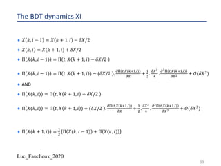
![Luc_Faucheux_2020
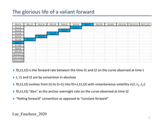
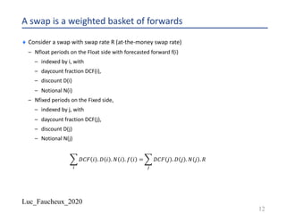
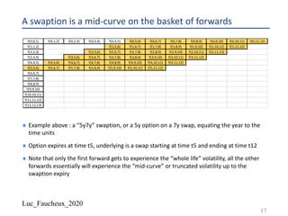
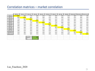
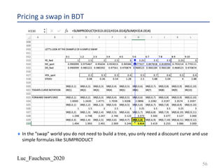
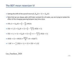
A swap rate is a weighted basket of forward rates
¨ At-the-money swap rate equation: ∑) 𝐷𝐶𝐹 𝑖 . 𝐷 𝑖 . 𝑁 𝑖 . 𝑓 𝑖 = ∑* 𝐷𝐶𝐹 𝑗 . 𝐷 𝑗 . 𝑁 𝑗 . 𝑅
¨ Above equation is valid at all times before the swap start, forwards and discount factors
being calculated on the then current discount curve the usual way, if the period I on the
float side starts at time ts(i) and ends at time te(i), and the forward is “aligned” with the
period (no swap in arrears or CMS like)
¨ 𝑅(𝑡) = ∑) 𝐷𝐶𝐹 𝑖 . 𝐷 𝑖 . 𝑁 𝑖 . 𝑓 𝑡, 𝑡𝑠 𝑖 , 𝑡𝑒(𝑖) /[∑* 𝐷𝐶𝐹 𝑗 . 𝐷 𝑗 . 𝑁 𝑗 ]
¨ “frozen numeraire” approximation, expand above equation in first order in forward rates but
keeping the discount factors constant
¨ 𝑑𝑅(𝑡) = ∑) 𝐷𝐶𝐹 𝑖 . 𝐷 𝑖 . 𝑁 𝑖 . 𝑑𝑓 𝑡, 𝑡𝑠 𝑖 , 𝑡𝑒(𝑖) /[∑* 𝐷𝐶𝐹 𝑗 . 𝐷 𝑗 . 𝑁 𝑗 ]
¨ Taking the square of the above yields the instantaneous volatility of the swap rate
¨ Λ+
" . 𝑑𝑡 =< 𝑑𝑅" >=
∑)! ∑)" 𝐷𝐶𝐹 𝑖1 . 𝐷 𝑖1 . 𝑁 𝑖1 . 𝐷𝐶𝐹 𝑖2 . 𝐷 𝑖2 . 𝑁 𝑖2 . < 𝑑𝑓 𝑖1 . 𝑑𝑓 𝑖2 > /
[∑*! ∑*" 𝐷𝐶𝐹 𝑗1 . 𝐷 𝑗1 . 𝑁 𝑗1 𝐷𝐶𝐹 𝑗2 . 𝐷 𝑗2 . 𝑁 𝑗2 ]
13](https://image.slidesharecdn.com/lf2020trees-200531142700/85/Lf-2020-trees-13-320.jpg)
![Luc_Faucheux_2020
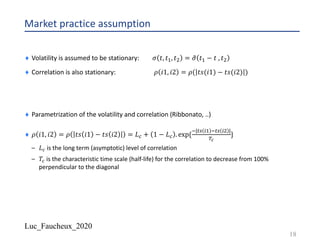
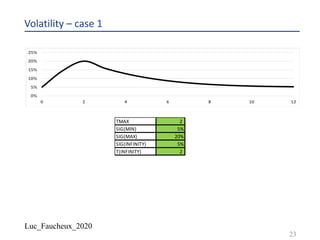
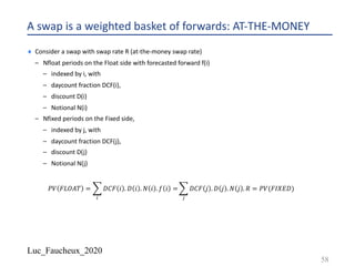
A swap rate is a weighted basket of forward rates
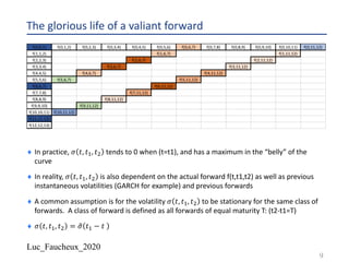
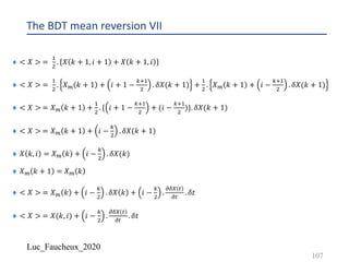
¨ instantaneous volatility of the swap rate
¨ Λ+
"
. 𝑑𝑡 =< 𝑑𝑅" >=
∑)! ∑)" 𝐷𝐶𝐹 𝑖1 . 𝐷 𝑖1 . 𝑁 𝑖1 . 𝐷𝐶𝐹 𝑖2 . 𝐷 𝑖2 . 𝑁 𝑖2 . < 𝑑𝑓 𝑖1 . 𝑑𝑓 𝑖2 > /
[∑*! ∑*" 𝐷𝐶𝐹 𝑗1 . 𝐷 𝑗1 . 𝑁 𝑗1 𝐷𝐶𝐹 𝑗2 . 𝐷 𝑗2 . 𝑁 𝑗2 ]
¨ Where 𝑑𝑓 𝑖1 = 𝑑𝑓 𝑡, 𝑡𝑠 𝑖1 , 𝑡𝑒(𝑖1) and 𝑑𝑓 𝑖2 = 𝑑𝑓 𝑡, 𝑡𝑠 𝑖2 , 𝑡𝑒(𝑖2)
¨ In abbreviated notation
¨ < 𝑑𝑓 𝑖1 . 𝑑𝑓 𝑖2 >= 𝜎 𝑖1 . 𝜎 𝑖2 . 𝜌 𝑖1, 𝑖2 . 𝑑𝑡
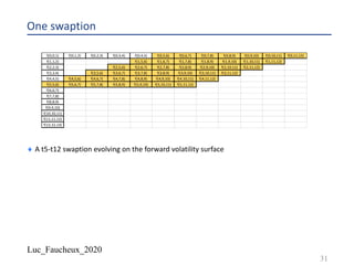
¨ So to calculate the instantaneous volatility of the swap rate you need the instantaneous
volatility of each forward BUT ALSO the instantaneous correlation matrix between the
forward constituting the weighted basket.
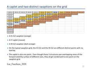
14](https://image.slidesharecdn.com/lf2020trees-200531142700/85/Lf-2020-trees-14-320.jpg)
![Luc_Faucheux_2020
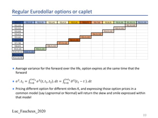
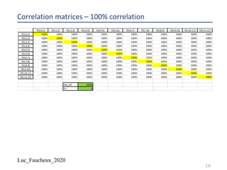
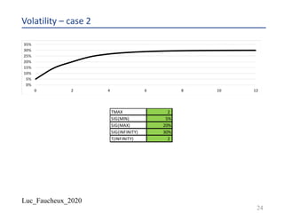
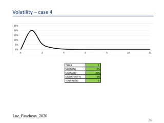
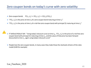
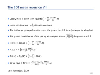
Parametrization of the volatility
¨ Usually assume a bell shape, with a maximum and a long term asymptote, with simple
analytical expression in order to integrate easily, and have numerically stable calibration
(sensitivity of the parameters to the market input are well behaved)
¨ We choose the following
– .𝜎 0 = .𝜎$%&
– .𝜎 ∞ = .𝜎'
– .𝜎 𝑇$() = .𝜎$()
– If 𝑡 < 𝑇$(), we use .𝜎*
𝑡 = .𝜎$%&
*
+ .𝜎$()
*
− .𝜎$%&
*
∗ (
+
,!"#
)
– If 𝑡 >= 𝑇$(), we use .𝜎*
𝑡 = .𝜎$()
*
+ .𝜎'
*
− .𝜎$()
*
∗ [1 − exp
- +-,!"#
,$
]
22](https://image.slidesharecdn.com/lf2020trees-200531142700/85/Lf-2020-trees-22-320.jpg)


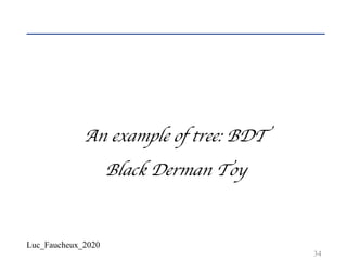

![Luc_Faucheux_2020
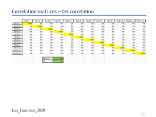
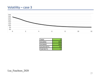
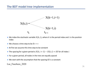
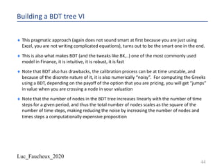
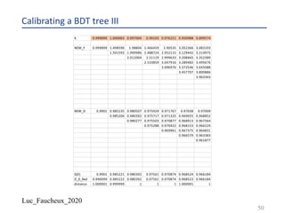
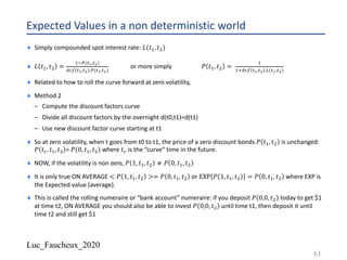
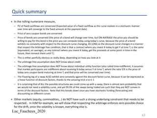
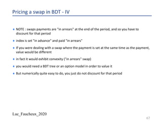
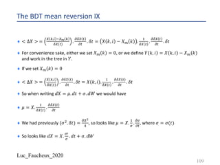
Building a BDT tree IV
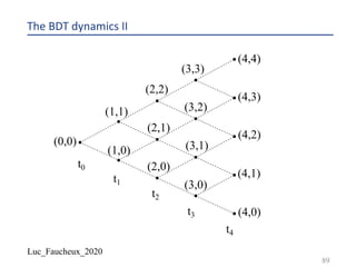
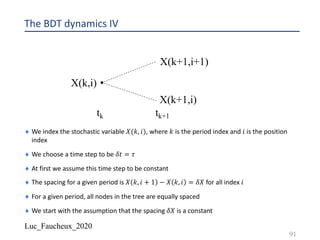
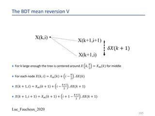
¨ We create a grid of forward yields 𝑋(𝑘, 𝑖)
¨ We chose for the “bottom” value 𝑋 𝑘, 0 =
3(#&,#&'!)
(!2
((&)
+
)^(1)
, where 𝑉(𝑘) is the volatility input
¨ The idea is to start with a distribution of forwards centered around the input one 𝑓(𝑡1, 𝑡1-!)
and with a standard deviation that will be close to the volatility input
¨ Each successive value for a given period going up the nodes in the tree is given by
¨ 𝑋 𝑘, 𝑖 + 1 = 𝑋 𝑘, 𝑖 . [1 + 𝑉 𝑘 ]1
42
Y_fwd 1 1.498501 1.994013 2.488784 2.97612 3.209678 3.427392
1.501499 2.005996 2.51125 3.024024 3.290726 3.573885
2.01805 2.533919 3.072699 3.373821 3.72664
2.556793 3.122158 3.459014 3.885924
3.172413 3.546359 4.052015
3.635909 4.225206
4.405799](https://image.slidesharecdn.com/lf2020trees-200531142700/85/Lf-2020-trees-42-320.jpg)


![Luc_Faucheux_2020
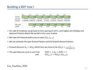
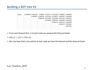
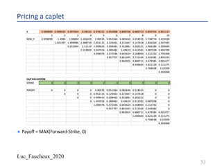
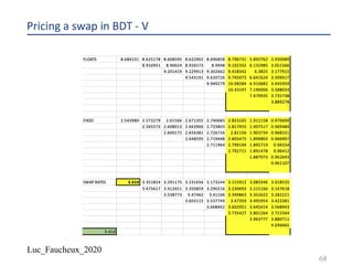
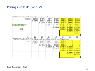
Standard Swap periods
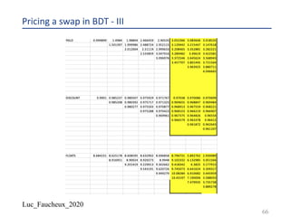
¨ On the fixed side, coupon payment at the end of the period
– Period start date (psj)
– Adjusted period start date (psj_adj)
– Period end date (pej)
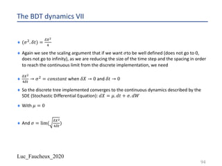
– Adjusted period end date (pej_adj)
– Payment date (pmj)
– PV of a period 𝑃𝑉 𝑗 = 𝐷𝐶𝐹 𝑗 . 𝐷 𝑗 . 𝑁 𝑗 . 𝑅 = 𝐷𝐶𝐹 𝑝𝑠𝑗./-, 𝑝𝑒𝑗_𝑎𝑑𝑗 . 𝐷 𝑝𝑚- . 𝑁 𝑗 . 𝑅
¨ On the float side, floating rate sets at the beginning of the period, and pays at the end (Libor in advance or
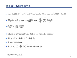
standard Libor swap, as opposed to Libor in arrears)
– PV of a period (swaplet) 𝑃𝑉 𝑖 = 𝐷𝐶𝐹 𝑖 . 𝐷 𝑖 . 𝑁 𝑖 . 𝑓 𝑖
– 𝐷𝐶𝐹 𝑖 = 𝐷𝐶𝐹 𝑝𝑠𝑖./-, 𝑝𝑒𝑖./- and 𝐷 𝑖 = 𝐷(𝑝𝑚𝑖)
– 𝐷 𝑝𝑒𝑖 = 𝐷 𝑝𝑠𝑖 ∗
0
01234 56,,58, .:(,)
or
– 𝐷𝐶𝐹 𝑝𝑒𝑖, 𝑝𝑠𝑖 . 𝑓 𝑖 = [1 −
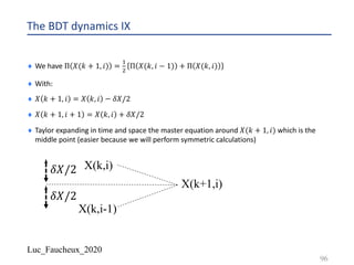
2 58,
2 56,
]
59](https://image.slidesharecdn.com/lf2020trees-200531142700/85/Lf-2020-trees-59-320.jpg)
![Luc_Faucheux_2020
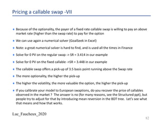
Floating leg of a swap
¨ A floating swaplet pays 𝐷𝐶𝐹 𝑖 . 𝑁 𝑖 . 𝑓 𝑖 and its PV is 𝑃𝑉 𝑖 = 𝐷𝐶𝐹 𝑖 . 𝐷 𝑖 . 𝑁 𝑖 . 𝑓 𝑖
¨ Where 𝐷𝐶𝐹 𝑝𝑒𝑖, 𝑝𝑠𝑖 . 𝑓 𝑖 = [1 −
2 58,
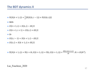
2 56,
]
¨ We know from the fixed rate leg that < 𝐷 𝑖 >= 𝐷 𝑖 , but what about < 𝐷 𝑖 . 𝑓 𝑖 > ?
¨ Note, to be exact < 𝐷 𝑖 >= 𝐷 𝑖 should really read ∏?#BC?$
𝐸𝑋𝑃{𝑡@, 𝑑(𝑡@, 𝑡@ + 1)}, where
𝐸𝑋𝑃 𝑡@, 𝑑 𝑡@, 𝑡@ + 1 is the expected value of the overnight discount between the time (tc) and (tc+1),
observed up until time tc (because it drops off the curve after tc, and before tc, no matter where you
observe it, its expected value is equal to today’s value)
¨ 𝐸𝑋𝑃 𝑡@, 𝑑 𝑡@, 𝑡@ + 1 = 𝐸𝑋𝑃 𝑡 < 𝑡@, 𝑑 𝑡@, 𝑡@ + 1 = 𝑑(𝑡@ + 1)
¨ Back to < 𝐷 𝑖 . 𝑓 𝑖 > , there is a little trick
63](https://image.slidesharecdn.com/lf2020trees-200531142700/85/Lf-2020-trees-63-320.jpg)

![Luc_Faucheux_2020
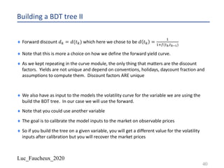
Legs of a swap in arrears
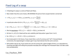
¨ A fixed leg of a swap is a series of fixed cash flows that pays
¨ 𝐷𝐶𝐹 𝑖 . 𝑁 𝑖 . 𝑆𝑅
¨ And its PV is:
¨ 𝐷𝐶𝐹 𝑖 . 𝑁 𝑖 . 𝑆𝑅. 𝐷(𝑖 − 1)
¨ A floating swaplet “in arrears” pays:
¨ 𝐷𝐶𝐹 𝑖 . 𝑁 𝑖 . 𝑓 𝑖
¨ and its PV is:
¨ 𝑃𝑉 𝑖 = 𝐷𝐶𝐹 𝑖 . 𝐷 𝑖 − 1 . 𝑁 𝑖 . 𝑓 𝑖
¨ Where 𝐷𝐶𝐹 𝑝𝑒𝑖, 𝑝𝑠𝑖 . 𝑓 𝑖 = [1 −
2 58,
2 56,
]
71](https://image.slidesharecdn.com/lf2020trees-200531142700/85/Lf-2020-trees-71-320.jpg)
![Luc_Faucheux_2020
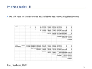
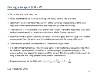
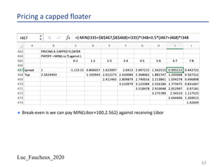
Floating leg of an “in arrears” swap
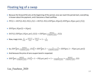
¨ Because the forward f(i) sets at the beginning of the period, once we reach the period start, everything
is known about the payment, and it becomes a fixed cashflow.
¨ 𝑃𝑉 𝑖 = 𝐷𝐶𝐹 𝑖 . 𝐷 𝑖 − 1 . 𝑁 𝑖 . 𝑓 𝑖 = 𝐷𝐶𝐹 𝑖 . 𝑁 𝑖 . 𝐸𝑋𝑃 𝑝𝑠𝑖, 𝐷 𝑝𝑠𝑖 . 𝐸𝑋𝑃{𝑝𝑠𝑖, 1. 𝑓 𝑖 }
¨ 𝐸𝑋𝑃 𝑝𝑠𝑖, 𝐷 𝑝𝑠𝑖 = 𝐷(𝑝𝑠𝑖)
¨ 𝐷𝐶𝐹 𝑖 . 𝐸𝑋𝑃 𝑝𝑠𝑖, 1. 𝑓 𝑖 = 𝐸𝑋𝑃{𝑝𝑠𝑖, 𝐷𝐶𝐹 𝑖 . 𝑓 𝑖 }
¨ Where 𝐷𝐶𝐹 𝑝𝑒𝑖, 𝑝𝑠𝑖 . 𝑓 𝑖 = [1 −
2 58,
2 56,
]
¨ Now, magic trick,
D
01D
=
D10=0
01D
=
01D=0
01D
= 1 −
0
01D
, but that gets us nowhere
¨ So, 𝐸𝑋𝑃 𝑝𝑠𝑖, 𝐷𝐶𝐹 𝑖 . 𝑓 𝑖 = 𝐸𝑋𝑃 1 −
2 58,
2 56,
¨ This has not only a timing difference but a ratio, and we all know that 𝐸𝑋𝑃
0
D
<> 1/𝐸𝑋𝑃(𝑥)
¨ This can be done through the Taylor expansion (or also Jensen inequality)
¨ This is the famous Swap in arrears convexity trade of May 1995 (story time)
73](https://image.slidesharecdn.com/lf2020trees-200531142700/85/Lf-2020-trees-73-320.jpg)


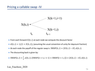


![Luc_Faucheux_2020
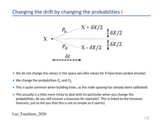
Changing the drift by changing the probabilities IV
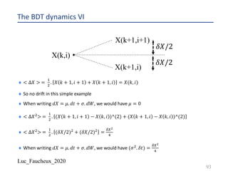
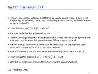
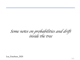
¨ So we match the process: 𝑑𝑋 = 𝑎. 𝑑𝑡 + 𝜎. 𝑑𝑊
¨ 𝛿𝑋 = 2𝜎. 𝛿𝑡!/"
¨ 𝜀 =
E
"=
𝛿𝑡!/"
¨ WAIT A MINUTE you should say, 𝜀 is only a number, not a complicated formula:
¨ 𝜀 =
E
"=
𝛿𝑡!/"
¨ 𝑎 is a drift and so scales as [
9
#
]
¨ 𝜎 is a volatility and so scales as [
9
#!/+], or easier 𝜎". [𝑡]scales as [𝑋"]
¨ SO.. 𝜀 scales as [
9
#
].
#
!
+
9
. [𝑡!/"] which is dimensionless and a number indeed !!
123](https://image.slidesharecdn.com/lf2020trees-200531142700/85/Lf-2020-trees-123-320.jpg)


![Luc_Faucheux_2020
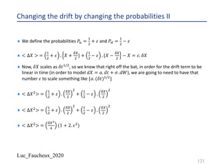
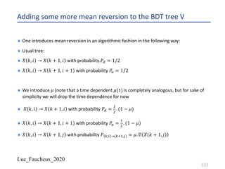
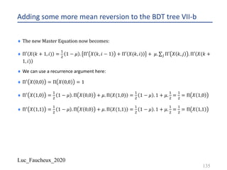
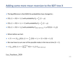
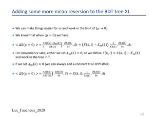
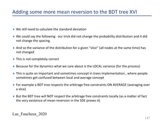
Adding some more mean reversion to the BDT tree XII
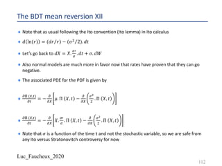
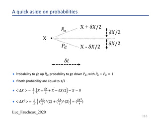
¨ In the limit of small 𝜇:
¨ < ∆𝑋 > =< 𝑋12!|𝑋(𝑘, 𝑖) > − 𝑋(𝑘, 𝑖)
¨ < 𝑋 > =< 𝑋 𝜇 = 0 >. 1 − 𝜇 + 𝜇. ∑*$%
*$12!
𝑋 𝑘 + 1, 𝑗 . Π 𝑋(𝑘 + 1, 𝑗)
¨ < ∆𝑋 > = < ∆𝑋 𝜇 = 0 >. 1 − 𝜇 + 𝜇. 𝛿 < ∆𝑋 >
¨ With 𝛿 < ∆𝑋 > = ∑*$%
*$12!
{𝑋 𝑘 + 1, 𝑗 − 𝑋 𝑘, 𝑖 }. Π 𝑋(𝑘 + 1, 𝑗)
¨ Or again :
¨ 𝛿 < ∆𝑋 > = [∑*$%
*$12!
𝑋 𝑘 + 1, 𝑗 . Π 𝑋 𝑘 + 1, 𝑗 − 𝑋 𝑘, 𝑖 ]
¨ Since: ∑*$%
*$12!
𝑋 𝑘, 𝑖 . Π 𝑋 𝑘 + 1, 𝑗 = 𝑋 𝑘, 𝑖 . ∑*$%
*$12!
Π 𝑋 𝑘 + 1, 𝑗 = 𝑋 𝑘, 𝑖
143](https://image.slidesharecdn.com/lf2020trees-200531142700/85/Lf-2020-trees-143-320.jpg)
![Luc_Faucheux_2020
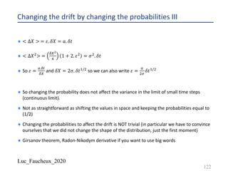
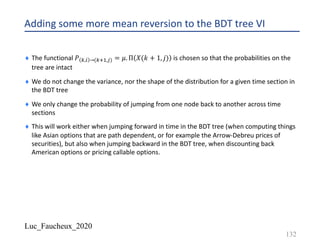
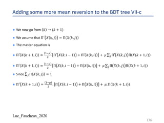
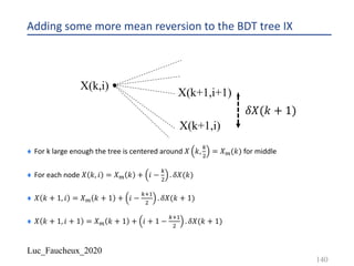
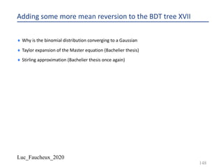
Adding some more mean reversion to the BDT tree XIII
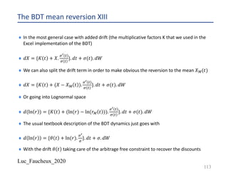
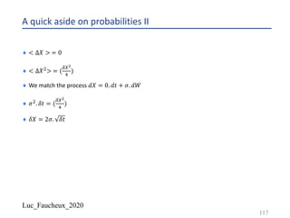
¨ We now have:
¨ < ∆𝑋 > = < ∆𝑋 𝜇 = 0 >. 1 − 𝜇 + 𝜇. 𝛿 < ∆𝑋 >
¨ 𝛿 < ∆𝑋 > = [∑*$%
*$12!
𝑋 𝑘 + 1, 𝑗 . Π 𝑋 𝑘 + 1, 𝑗 − 𝑋 𝑘, 𝑖 ]
¨ 𝛿 < ∆𝑋 > = [𝑋?(𝑘 + 1) − 𝑋 𝑘, 𝑖 ]
¨ Remember that:
¨ 𝑋? 𝑘 + 1 = ∑*$%
*$12!
𝑋 𝑘 + 1, 𝑗 . Π 𝑋 𝑘 + 1, 𝑗
¨ In the limit of a dense tree 𝑋? 𝑘 = 𝑋(𝑘,
1
"
)
¨ And for each node 𝑋 𝑘, 𝑖 = 𝑋? 𝑘 + 𝑖 −
1
"
. 𝛿𝑋(𝑘)
144](https://image.slidesharecdn.com/lf2020trees-200531142700/85/Lf-2020-trees-144-320.jpg)
![Luc_Faucheux_2020
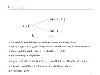
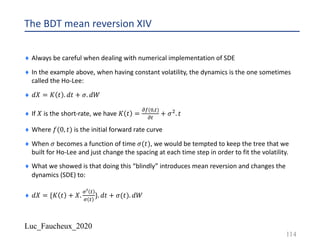
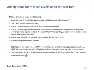
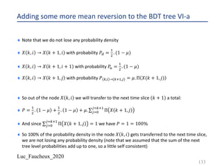
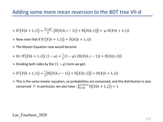
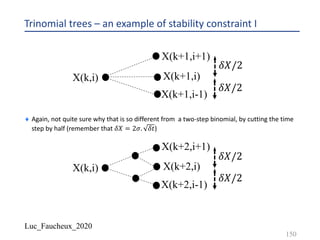
Adding some more mean reversion to the BDT tree XIV
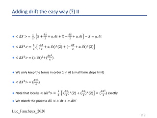
¨ < ∆𝑋 > = < ∆𝑋 𝜇 = 0 >. 1 − 𝜇 + 𝜇. [𝑋?(𝑘 + 1) − 𝑋 𝑘, 𝑖 ]
¨ Again we take the liberty of setting 𝑋? 𝑘 + 1 = 𝑋? 𝑘 = 0
¨ (as we can always impose a constant drift later)
¨ And so : < ∆𝑋 > = 𝑋 𝑘, 𝑖 .
!
89 #
.
;89 #
;#
. 𝛿𝑡. 1 − 𝜇 − 𝜇. 𝑋 𝑘, 𝑖
¨ This looks almost like what we are after
¨ We need to check that the units are correct and consistent between the two terms, in
particular we look to be missing a 𝛿𝑡 factor in the second term
¨ Also we worked in the limit (𝜇 → 0) but we know that the BDT construction is algorithmic in
nature, so we are missing the cross-terms and higher order terms, we will need to be
conscious of that
¨ On the other hand we are trying to get the SDE, which is continuous limit, and not that
helpful, because we are using BDT anyways, and not looking for closed form solutions
145](https://image.slidesharecdn.com/lf2020trees-200531142700/85/Lf-2020-trees-145-320.jpg)
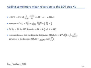


![Luc_Faucheux_2020
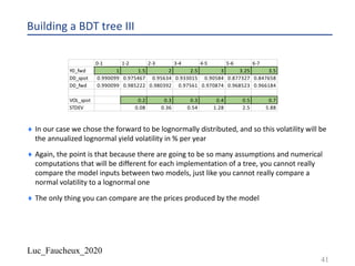
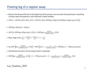
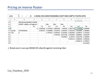
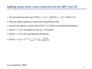
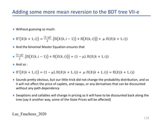
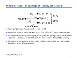
Trinomial trees – an example of stability constraint VI
¨ The solution is then:
¨ 𝑃A = 1 − {(𝛼. 𝛿𝑡)"+𝜎". 𝛿𝑡}.
89
"
-"
¨ 𝑃L =
!
"
. [
"M.8#
89
+ {(𝛼. 𝛿𝑡)"+𝜎". 𝛿𝑡}.
89
"
-"
]
¨ 𝑃K =
!
"
. [−
"M.8#
89
+ {(𝛼. 𝛿𝑡)"+𝜎". 𝛿𝑡}.
89
"
-"
]
¨ Note that it would seem sensible that all probabilities should be in [0,1]
¨ A negative probability in the tree is not necessarily a sign that something is wrong, but it is a
constraint that we would like to enforce (related to stability analysis)
155](https://image.slidesharecdn.com/lf2020trees-200531142700/85/Lf-2020-trees-155-320.jpg)


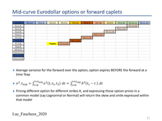
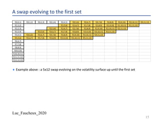
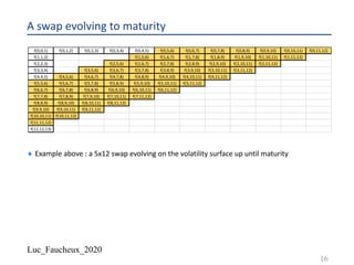
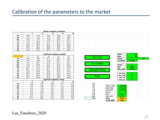
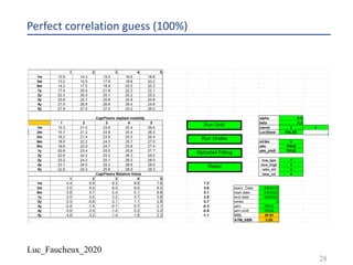
The document discusses various numerical methods in financial modeling, specifically focusing on binomial trees, Monte Carlo simulations, and forward rates. It contrasts recombining and non-recombining binomial trees in terms of their computational efficiency and arbitrage compliance, while also elaborating on the complexities of modeling forward rates and swaps. Additionally, it addresses volatility calculations for options and swaps, emphasizing their respective dependencies on the underlying forward rates and market conditions.


