This thesis examines lattice approximations for option pricing models similar to the Black-Scholes model. It covers the binomial and trinomial lattice models. The binomial model is introduced, including calculating prices of European and American options using risk-neutral probabilities. Various approaches for deriving the model parameters are discussed. Convergence of the binomial model to the Black-Scholes model under risk-neutral probabilities is shown. The trinomial model and its properties are also covered. Different variants of the binomial model are analyzed and compared.

![is a common algorithm for calculating the fair price of any option and this algorithm states
that the fair price of an option is its discounted expected payoff. When we talk about expected
value in simple cases, we know that it is the average or mean of a sample or population. But
finding expected values of some processes is not that easy. Moreover there are some contro-
versial questions. How to calculate this expected value? Is it always possible to calculate the
price of an option analytically? How should one translate mathematical formulas to computer
language? If it is not possible to calculate the price of an option analytically, which numerical
method should be used to estimate the price of the option? What is the error of estimations?
What are the definitions for different options and how does one calculate their payoffs? To
answer some of these questions, we will try to explain the basic definitions and ideas about
options and how to price them. This process is strongly related to our knowledge which we
have obtained by studying the Bachelor’s Program in Analytical Finance at Mälardalen Hög-
skola. We will go through the basic ideas which are vital for understanding the algorithm of
pricing options specifically in computer language and when we talk about simulating some
process for which we can find the result by numerical methods [6].
After our introduction, we will in Chapter 2 go through the concept of binomial models. We
will study how it is possible to price an option using a binomial tree. In the binomial model
Chapter, we will start with the definitions of payoff for European and American options [7],
which we have studied in the course "Introduction to Financial Mathematics". After that, we
will follow our process by studying some probability theorems and definitions [21] which are
essential for getting a good understanding for pricing options via the binomial model approach.
We obtained this knowledge in our "Probability" course. Then, using binomial approach, we
will try to explain how the price of American and European options can be calculated. At this
step, we will be able to analyze a binomial tree and we will have a system of equations with
some unknowns. We will continue our process by calculating them. Firstly, we will try to
find the value for risk-neutral probability [4], [7] by constructing a replicating portfolio. Here
we will get help from different literature like our knowledge from the courses "Stochastic
Processes" [12] and its lecture notes [14]. Secondly, we will derive the other unknowns in
our system of equations, namely up and down factors in full details and we will study the
CRR model (Cox, Ross and Rubinstein model) and its results [4]. After that, we will talk
about random walks and transition probabilities which will help us to derive the backward and
forward equations for pricing options [12],[14]. Consequently, we will discuss the formula for
pricing the option [7]. Finally, we will end Chapter 2, with some example which will show
how our process can be helpful to price options, especially when we deal with an American
Put option, in which early exercise on a predetermined date is possible.
In Chapter 3, we start to compare and contrast the behavior of a random variable, namely
stock price, in discrete and continuous time. Additionally, we will consider the result of Black
and Scholes [1] and Merton [15]. We know they assumed that the dynamic of risky security
prices follows a Geometric Brownian Motion. We will also follow Cox, Ross and Rubinstein
[4] approach to see how as well the sequence of the binomial model converges to Geometric
5](https://image.slidesharecdn.com/056831bc-2170-4601-b463-4525efb79d14-150711133700-lva1-app6892/85/Bachelor-Thesis-Report-7-320.jpg)
![Brownian Motion. To do so, we will start studying the sequence of the binomial model and
its convergence to normal distribution [12],[14],[21]. Then we will show how the sequence
of the binomial model converges to the Black-Scholes model under risk neutral probability
[12],[14]. After that, we will make a distinction between normal and log-normal random
variables. Moreover, we will discuss how stock prices can be treated as log-normal random
variables with normal-distribution and how it can be treated as a normal random variable with
log-normal distribution. In this part we do some interesting derivations using our knowledge
from calculus and probability [21], which are really useful for approximation of some variants
of binomial models to the Black-Scholes pricing formula.
In Chapter 4, we will study some different variants of binomial models. We have seen the
result and formula for some of these variants in our course "Analtical Finance I" [17], but
we will try to apply our knowledge to derive the final formulas in details. We will see that
for the binomial approach, we will always have two equations for expected value and variance
which, depending on our choice of normality or log-normality of our random variable (namely
stock price), can be approximated differently with different means and variances. Moreover,
we will see that we have a system of two equations and three unknowns. We will see that
for example Cox, Ross and Rubinstein [4] chose their third equation like ud = 1. In simple
cases, we introduce our third equation by ud = 1 or p = 1/2 and we will approximate the
binomial model in a way that the mean and the variance of our models converge to the Black-
Scholes formula. Then we will study some other models like Jarrow-Rudd model [10],[9],
Tian model [19], Trigeorgis model [20] and Leisen-Reimer model [13]. We will see how the
approximation of these different models works and what advantage and disadvantage each
model has. There are lots of other models which can be considered, but we will finish this
chapter by just considering the models that we have mentioned.
In Chapter 5, we will study the trinomial model. We start off with the basic principles of
the trinomial distribution. It is similar to the binomial distribution, but not as widely used.
Consequently there was less literature available that covered the subject but due to the simil-
arity with the binomial model, previous knowledge of probability theory and Wackerly [21],
the concept and properties of trinomial distribution is derived and explained. It is important
so that further parts can be understood.
Directly after the basics of trinomial distribution we study the paper of Boyle from 1988 [2]
because it extends Cox, Ross and Rubinstein approach of risk neutral valuation with jumps in
two directions (binomial model) into a model with jumps in three directions (trinomial model)
with the condition of risk neutral return which in the short term is the risk free interest rate.
The probabilities under this process are derived connecting mean and variance of discrete
and continuous distributions where the discrete functions are approximations of the lognormal
distribution of the underlying asset which is governed by a Geometric Brownian Motion. This
model will show that we have two constraints and five unknown parameters, giving no unique
parameters for the probabilities.
6](https://image.slidesharecdn.com/056831bc-2170-4601-b463-4525efb79d14-150711133700-lva1-app6892/85/Bachelor-Thesis-Report-8-320.jpg)
![The next section deals with risk neutral probability as well. We will examine if the replicating
portfolio can generate the contingent claim if three different movements on the underlying
asset are assumed (in contrast to two, which we examine in the binomial lattice). Since we used
Kijima [12] and the lecture notes from Stochastic Processes [14] for the replicating portfolio
in the binomial model, we find it appropriate to use it for the trinomial variant as well.
Another method for finding parameters suitable to generate contingent claims was established
by Kamrad and Ritchken in 1991 [11]. Their idea was to approximate the logarithm of the
random variable that describes the return of the underlying asset in one time step. Even here
the random variable is discretized in the trinomial lattice and the first two moments of the
continuous distribution is matched with those of the discrete distribution.
As we have seen we show several methods where the approximation of the continuous random
variable is done by a lattice approach. The next part however uses another method, namely the
explicit finite difference approach. We show how the partial derivatives in the Black-Scholes
formula can be discretized and further processed in order to find probability densities that
satisfy the partial differential equation. Originally Brennan and Schwartz [3] developed this
technique, but we studied the notes from Analytical Finance [17] and Hull [7] as well, because
the paper itself is structured in a complicated way. For easier understanding we even included
graphics in this part.
In the last part we try to find a connection between binomial and trinomial trees based on
an observation of one of the authors of this thesis that binomial lattices and trinomial lattices
overlap. As we investigated this connection further we found a paper by Derman et al from
1996 [5] which was really helpful and led to yet another discovery, namely that there are tree
models with constant volatility, called standard trees, and trees that are constructed in order
to match the volatility smile with varying volatility, called implied trees. We give a brief
explanation of this detection.
We found it reasonable as well to show the Black-Scholes formula and how it is derived. The
appendix covers this subject.
All sources that we have used are either published papers or text books, or lecture notes from
professors at Mälardalens Högskola. We had the great opportunity to download the papers
from Jstor through our university accounts. We find all references very reliable since they are
provided through academic sources and have educated many students and people working in
finance and economics, before us.
7](https://image.slidesharecdn.com/056831bc-2170-4601-b463-4525efb79d14-150711133700-lva1-app6892/85/Bachelor-Thesis-Report-9-320.jpg)
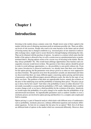
![Chapter 2
Binomial Model
In market the price of stocks move randomly. The price of stocks can go up, down or remain
constant between two time intervals. So, the movements of stock prices are stochastic pro-
cesses. In simple case we can consider a random walk with predefined length of movements.
We assume the price of stock can go up or down for a certain amount in each time interval
with the probability of p and 1− p respectively. This simple model is called Binomial model.
The price of stock at time zero is denoted by S0 and it is usual to denote the amount of in-
creasing by uS0 and the amount of decreasing by dS0. One can start from today, i.e., node one
at the time zero and build a binomial tree for a finite time interval. Figure 2.1 illustrates three
steps binomial tree graphically. It is obvious that the possible stock prices can be calculated
easily at any node. But, how to calculate the fair price of an option? As mentioned before the
discounted expected payoff must be considered. In binomial tree at any node we can count all
the possible paths to reach that specific node. And then we can formulate our expected payoff.
Instead of counting all possible way to reach a specific node we need to explain the formu-
lation of binomial expansion and binomial coefficient which can represent the probability of
reaching at any specific node at any step. But, first let start by the most important definitions
for option pricing and then we will continue by some probability theorems and definitions as
well as binomial expansion.
2.1 Payoff to European and American Options
Let us start with the definition of American and European options1 [7].
Definition 2.1.1. European Options are options which give the holder of the options the right,
but not the obligation, to exercise them at maturity.
1In the market there exist several different kinds of options, like Bermudan Options, which are a part of
nonstandard American options, Asian options, Currency Options, Swap Options, Barrier Options and ... [7]
8](https://image.slidesharecdn.com/056831bc-2170-4601-b463-4525efb79d14-150711133700-lva1-app6892/85/Bachelor-Thesis-Report-10-320.jpg)
![S0
S0u
S0d
S0u2
S0ud
S0d2
S0u3
S0u2d
S0ud2
S0d3
∆T
∆t ∆t ∆t
t0 t1 t2 T
Figure 2.1: Three Steps Binomial Tree
Definition 2.1.2. American Options are options which give the holder of the options the right,
but not obligation, to exercise them at any time up to maturity.
It can be proved that the price of an American put option must be greater or or equal to the
price of a European put option [7]. It can also be proved that the price of American call and
European call options is the same [7] under the condition that the underlying asset does not
pay dividends. As it was explained, the honest price for an option is its discounted expected
payoff. For discounting a price it is common to use the risk-free interest rate r with continuous
compounding. To explain it mathematically we can write:
Price = e−r∆T
E[payoff] (2.1)
To distinguish between the options we can define their payoffs as follow [7]:
Long Call:
payoff = max{ST −K,0}
Short Call:
payoff = −max{ST −K,0}
Long Put:
payoff = max{K −ST ,0}
9](https://image.slidesharecdn.com/056831bc-2170-4601-b463-4525efb79d14-150711133700-lva1-app6892/85/Bachelor-Thesis-Report-11-320.jpg)
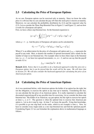
![f0
fu
fd
fu2
fud
fd2
fu3
fu2d
fud2
fd3
∆t ∆t ∆t
t0 t1 t2 T
Figure 2.2: Three Steps Binomial Tree
Short Put:
payoff = −max{K −ST ,0}
where K is the strike price and ST is the stock price at maturity. As we can see, the payoff
equations for both European and American options are the same. Let us denote the payoff
at each node by f with its path indexes. The procedure is explained in Figure 2.2. Let us
furthermore equip ourselves with some probability theorems and definitions to calculate the
price of an option in the binomial model.
2.2 Binomial Expansion
In this part, we will study some related important theorems and definitions [21].
Definition 2.2.1. Let p and q be any real number, then Binomial Expansion of (p+q)n is:
(p+q)n
=
n
∑
k=0
n
k
pn
qn−k
(2.2)
where the Binomial Coefficients are:
n
k
=
n!
k!(n−k)!
(2.3)
10](https://image.slidesharecdn.com/056831bc-2170-4601-b463-4525efb79d14-150711133700-lva1-app6892/85/Bachelor-Thesis-Report-12-320.jpg)
![The binomial coefficients are useful for calculating the probability distribution in a binomial
tree. Let us continue with the next theorem [21].
Theorem 2.2.1. For any discrete probability distribution, the following must be true:
1. 0 ≤ p(y) ≤ 1 , for all y
2. ∑y p(y) = 1 , where the summation is over all values of y with nonzero probability.
The definition for binomial distribution is [21]:
Definition 2.2.2. A random variable K is said to have a Binomial Distribution based on n
trails with success probability p if and only if
p(k) =
n
k
pn
(1− p)n−k
(2.4)
where
k = 0,1,2,...,n and 0 ≤ p ≤ 1
The formula (2.4) defines the probability function for a discrete random variable. Considering
Theorem 2.2.1 we say q = 1 − p and we will use it to calculate the price of some options.2
Moreover, the following definition will help us to calculate the mean or expected value of a
discrete random variable [21].
Definition 2.2.3. Let Y be a discrete random variable with probability function p(y). Then
the Expected Value of Y, E(Y), is defined to be
E(Y) = ∑
y
yp(y) (2.5)
if the above series is absolutely convergent.
Finally, we can find the variance of a discrete random variable using the following theorem
[21].
Theorem 2.2.2. Let Y be a discrete random variable with probability function p(y) and mean
E(Y) = µ; then
V(Y) = σ2
= E (Y − µ)2
= E Y2
− µ2
(2.6)
Remark 2.2.1. Using Definition 2.2.3 we can see that E Y2 = ∑y y2 p(y).
These theorems and definitions will play a considerable role in lattice approaches.
2The mean in the discrete binomial distribution is µ = np and the variance is σ2 = np(1− p) [21].
11](https://image.slidesharecdn.com/056831bc-2170-4601-b463-4525efb79d14-150711133700-lva1-app6892/85/Bachelor-Thesis-Report-13-320.jpg)
![optimal{fu2} = max fu2,e−r∆t
[pfu3 +(1− p)fu2d]
= max (K −ST ,0),e−r∆t
[pfu3 +(1− p)fu2d]
optimal{ fud} = max fud,e−r∆t
[pfu2d +(1− p)fud2]
= max (K −ST ,0),e−r∆t
[pfu2d +(1− p)fud2]
If we continue doing so, we will be able to calculate the optimal values in all nodes and go back
one more time. Then we will use the optimal values of the previous nodes to calculate their
discounted expected payoff. We continue doing so until we reach time zero. The discounted
expected payoff at time zero will be the fair price of the American option.
PA = e−r∆t
[p×optimal{ fu}+q×optimal{fd}]
Now we almost cover every important aspect of the binomial tree. But we still need to know
more about the probability p and the u and d factors.
2.5 Risk-Neutral Probability (The Cox-Ross-Rubinstein Model)
Consider a financial market containing of two different securities, a deterministic bond and a
stock which follows a stochastic process.We assume that the market is free of arbitrage. It is
possible to prove that the stock price is its discounted expected payoff [7],[17].
In general:
S(t) = e−rT
Ep∗
[S(T)]
where p∗ is called the Risk-Neutral Probability measure or the equivalent martingale measure.
Risk-neutral probability measure in the binomial model was originally calculated by Cox,
Ross and Rubinstein. They calculated p∗ as [4]:
p∗
=
er∆t −d
u−d
(2.7)
where u and d are up and down factors in the binomial tree, r is the risk-free interest rate and
∆t is the time between each two steps in the binomial tree.
Using Definition 2.2.3 and (2.5) the expected stock price in the two step-Binomial tree at time
T can be calculated as [7]:
E[S(T)] = p∗
S0u+(1− p∗
)S0d (2.8)
E[S(T)] = p∗
S0(u−d)+S0d (2.9)
Substituting (2.7) in (2.9) we will get:
E[(S(T)] = S0erT
⇒ S0 = e−rT
E[S(T)] (2.10)
The current result tells us that in a risk neutral world, the expected return on a stock is equal
to the risk-free interest rate.
13](https://image.slidesharecdn.com/056831bc-2170-4601-b463-4525efb79d14-150711133700-lva1-app6892/85/Bachelor-Thesis-Report-15-320.jpg)
![Calculating Risk-Neutral Probability p∗
Consider a market which consists of two types of financial instruments, bonds and stocks.
Moreover, there is no possibility of arbitrage. We know that bonds guarantee a certain amount
of profit in a specific time period, but the return on the stock is a stochastic process. To begin
with, we can write the process of these two securities in mathematical language as follows
[12],[14],[17]:
B(t) =
er∆t = 1 ,for t = t0 = 0
er∆t ,for t = t1 = T
B represents bonds with deterministic processes and their value at time zero will be one unit
of amount of money. At time T it will be their initial value plus the risk-free interest rate
continuous compounded and 0 ≤ t ≤ T.
As we discussed it previously, stocks follow a stochastic process and this will be as fol-
lows:
S(t) =
S0 ,for t = 0
S(T) ,for t = T
Before going further, it might be crucial to explain our portfolio. Our portfolio is simply our
properties. We have invested our money in two categories: stocks and bonds. Let us say
that we have decided to invest x percent of our money in bonds and y percent of our money
in stocks. x and y can get negative values since its possible to short one of the securities to
long the other, but under condition x +y = 1. Let us call our portfolio h. So the value of our
portfolio at time t is:
V(t,h) = xB(t)+yS(t)
which represents the value process of portfolio h. We can expand the expected value of the
portfolio of bonds and stocks at time t:
E[V(t,h)] =
xB(0)+yS(0) ,for t = 0
xB(T)+yE[S(T)] ,for t = T
which can be simplified as:
E[V(t,h)] =
x+yS0 ,for t = 0
xer∆t +yE[S(T)] ,for t = T
We have already discussed the possible outcomes of S(t) in the one step binomial model. So
the value process at time t = T can be rewritten as:
V(t,h) =
xer∆t +yS0u ,if stock goes up with probability p
xer∆t +yS0d ,if stock goes down with probability 1-p
Since the proportions of x and y are arbitrary, we can choose them in such a way that the
14](https://image.slidesharecdn.com/056831bc-2170-4601-b463-4525efb79d14-150711133700-lva1-app6892/85/Bachelor-Thesis-Report-16-320.jpg)
![value of each possible outcome will be equal to value of portfolio at the end of the portfolio
[12],[14]. This yields:
fu = xer∆t
+yS0u (2.11)
fd = xer∆t
+yS0d (2.12)
We have already seen how to calculate fu and fd for different options. Solving (2.12) and
(2.11) for x and y we will get:
y =
fu − fd
S0(u−d)
(2.13)
Substituting (2.13) to either (2.12) or (2.11) yield:
x =
ufd −d fu
er∆t(u−d)
We already know that in two steps binomial tree the following equation holds:
f0 = e−r∆t
[pfu +(1− p)fd] (2.14)
Moreover, if we substitute the value of x and y into he value process formula for our portfolio
h at time zero we will obtain:
V(0,h) = f0 = x+yS0 =
ufd −d fu
er∆t(u−d)
+
fu − fd
S0(u−d)
S0
= f0 = e−r∆t er∆t −d
u−d
fu +
u−er∆t
u−d
fd (2.15)
comparing (2.14) and (2.15) shows the value of p and 1− p. Here we had a two steps binomial
tree so ∆t = t1 −t0 = T −0 = T, but for a binomial tree with more than two steps it is better
to denote the change in time for each step by ∆t. The risk-neutral probability measure will be
[4]:
p∗
=
er∆t −d
u−d
1− p∗
=
u−er∆t
u−d
d ≤ r ≤ u (2.16)
Remark 2.5.1. The condition d ≤ r ≤ u will guarantee that our portfolio is free of arbitrage,
our neutral probabilities will lie between zero and one, and we will not obtain zero in the
denominator. It is easy to see that the sum of two fractions will be exactly one, and this is what
we expected. Additionally, this formula tells us, in a risk-neutral world, the expected return
on a stock must be equal to the risk-free interest rate [4].
2.6 Volatility with u and d factors
In practice, the volatility of a financial security can be estimated by the historical market data.
Thus, it is logical to calculate the u and d factors which are related to such volatility [7].
15](https://image.slidesharecdn.com/056831bc-2170-4601-b463-4525efb79d14-150711133700-lva1-app6892/85/Bachelor-Thesis-Report-17-320.jpg)
![These factors are calculated in different ways3, but we use the result proposed by Cox, Ross
and Rubinstein in 1979 [4] which are as follows:
u = eσ
√
∆t
, d = e−σ
√
∆t
(2.17)
Calculating u and d factors
To calculate up and down factors we can consider two significantly different ways. One ap-
proach is having our stochastic process in continuous time and the second approach is con-
sidering our stochastic process with jump diffusion. In the first case, the length of one time
intervals plays a vital role for our process. But in second case the movement of the random
variable will be more smooth, and it can have sudden discontinuous jumps or changes [4]. We
will go through the first approach. We have seen this approach and its result in [4],[7] but there
is no full detailed derivation of up and down factors in neither references [4],[7]. We will start
by following a corollary.
Corollary 2.6.1. The up and down factors in discrete time are given by [4]:
u = eσ
√
∆t
d = e−σ
√
∆t
.
Proof. To begin with, let’s consider a two-step binomial tree. We know that the possible stock
prices at time t = T are :
ST =
S0u ,if stock goes up with probability p
S0d ,if stock goes down with probability 1-p
Using Definition 2.2.3 the expected value will be:
E[ST ] = p∗
S0u+(1− p∗
)S0d
Recall equations (2.8) and (2.10) and consider the fact that in a risk neutral world the drift
coefficient is equal to the risk-free interest rate, i.e., µ = r (See [4],[7]).
E[ST ] = p∗
S0u+(1− p∗
)S0d = S0eµ∆t
Dividing by S0 we will get the first equation to calculate u and d.
E[ST /S0] = p∗
u+(1− p∗
)d = eµ∆t
(2.18)
Using Theorem 2.2.2 and (2.6), the variance will be
V[ST ] = E[S2
T ]−(E[ST ])2
3It is possible to calculate u and d factors with normal distribution, log-normal distribution, mixed normal/log-
normal distribution, the Cox-Ross-Rubenstein model, the Second order Cox-Ross-Rubenstein, the Jarrow-Rudd
model, the Tian model, the Trigeorgis model, ...[17]
16](https://image.slidesharecdn.com/056831bc-2170-4601-b463-4525efb79d14-150711133700-lva1-app6892/85/Bachelor-Thesis-Report-18-320.jpg)
![V[ST /S0] =
1
S2
0
V[ST ] = p∗
u2
+(1− p∗
)d2
−e2µ∆t
In a small time interval ∆t, the variance must be equal to σ2∆t, so we will get the second
equation [7]
p∗
u2
+(1− p∗
)d2
−e2µ∆t
= σ2
∆t (2.19)
Substituting the values of p∗ and (1− p∗) from (2.16) to (2.19) we will get:
σ2
∆t =
eµ∆t −d
u−d
u2
+
u−eµ∆t
u−d
d2
−e2µ∆t
=
eµ∆t(u2 −d2)−ud(u−d)
u−d
−e2µ∆t
=
eµ∆t(u−d)(u+d)−ud(u−d)
u−d
−e2µ∆t
= eµ∆t
(u+d)−ud −e2µ∆t
(2.20)
Now, we have two equations and three unknowns. To solve this we can consider Cox, Ross
and Rubinstein approach where they consider a recombining tree and they put ud = 1 [4].
By letting ud = 1 we will have two equations for the expected value and variance and two
unknowns, u and d. Solving (2.20) will give us the result for u and d in formula (2.17).
Let’s try to do a little algebra and see how it is possible to solve this. To begin with, we know
that the Maclaurin expansion for exponential functions is:
ex
=
∞
∑
n=0
xn
n!
= 1+x+
1
2
x2
+
1
3!
x3
+... (2.21)
using (2.21) and ignoring the terms of higher order than ∆t [7], we can introduce the following
equations:
eσ2∆t = 1+σ2∆t
eµ∆t = 1+ µ∆t
e2µ∆t = 1+2µ∆t
Substituting d = 1/u and solving (2.20) for u we will get:
u2
−
1+σ2∆t +e2µ∆t
eµ∆t
u+1 = 0
Let’s solve this quadratic equation, we introduce the notation b :
−b =
1+σ2∆t +e2µ∆t
eµ∆t
and solve the equation
u1,2 =
−b ±
√
b 2 −4
2
17](https://image.slidesharecdn.com/056831bc-2170-4601-b463-4525efb79d14-150711133700-lva1-app6892/85/Bachelor-Thesis-Report-19-320.jpg)
![Now let us calculate b :
−b =
1+σ2∆t +e2µ∆t
eµ∆t
=
1+σ2∆t
eµ∆t
+eµ∆t
=
eσ2∆t
eµ∆t
+eµ∆t
= e(σ2−µ)∆t
+eµ∆t
= [1+(σ2
− µ)∆t]+(1+ µ∆t) = 2+σ2
∆t
It follows:
b 2
−4 = (2+σ2
∆t)2
−4 = 4+4σ2
∆t +σ4
(∆t)2
−4 = 4σ2
∆t
so
u1,2 =
2+σ2∆t ±2σ
√
∆t
2
= 1±σ
√
∆t +
1
2
σ2
∆t
u1 = 1+σ
√
∆t + 1
2σ2∆t = eσ
√
∆t
u2 = 1−σ
√
∆t + 1
2σ2∆ = e−σ
√
∆t
Similarly, if we solve (2.20) for d:
d1 = 1−σ
√
∆t + 1
2σ2∆t = e−σ
√
∆t
d2 = 1+σ
√
∆t + 1
2σ2∆t = eσ
√
∆t
Since the condition d ≤ r ≤ u must be fulfilled, we can only accept the answers which satisfy
this condition. Thus d = d1 and u = u1. This result is the same as Cox-Ross-Rubinstein’s
(CRR) model [4], which is one of the most widely used models.
Now we will review an important part of Cox, Ross and Rubinstein’s paper [4]. Understanding
their approach will help us to further study the binomial model. Generally, the price of a stock
at the n-step binomial tree is determined by the following possible path on the binomial tree
[4]:
ST = um
dn−m
S0
If our random variable takes upward movements m times in n possible steps, then the random
variable takes n−m downward movements. Dividing both hand sides with S0 and taking the
logarithm yields [4]:
ln
ST
S0
= ln um
dn−m
= mlnu+(n−m)lnd
= mlnu+nlnd −mlnd = mln
u
d
+nlnd
18](https://image.slidesharecdn.com/056831bc-2170-4601-b463-4525efb79d14-150711133700-lva1-app6892/85/Bachelor-Thesis-Report-20-320.jpg)
![We calculate the expectation and consider the fact that we just have a random variable m here.
The expectation of a constant is its value [4]
E ln
ST
S0
= E mln
u
d
+nlnd
= E mln
u
d
+E [nlnd] = E[m]ln
u
d
+nlnd
Using Theorem 2.2.2 and (2.6), the variance of a random variable X can be calculated as
V[X] = E[X2]−(E[X])2
, so the variance will be:
V ln
ST
S0
= E mln
u
d
+nlnd
2
− E mln
u
d
+nlnd
2
= ln
u
d
2
E[m2
]−(E[m])2
= ln
u
d
2
V[m]
Since probability p∗ corresponds to up movements, the mean and variance of m will be
[4]
E[m] = np∗
,V[m] = np∗
(1− p∗
)
Thus the expected value and variance will be [4]:
E ln
ST
S0
= np∗
ln
u
d
+nln(d) = p∗
ln
u
d
+ln(d) n ≡ ˆµn
V ln
ST
S0
= ln
u
d
2
np∗
(1− p∗
) ≡ ˆσ2
n
We know that the length of each step is the length of time divided by steps in our binomial
tree. So, ∆t = t
n. If we have n big enough(n → ∞), we can choose u, d and p∗ in a way that
[4]:
lim
n→∞
p∗
ln
u
d
+ln(d) n = µt
lim
n→∞
ln
u
d
2
np∗
(1− p∗
) = σ2
t
Cox, Ross and Rubinstein showed that the possible values to satisfy these conditions are
[4]
u = eσ
√
∆t
,d = e−σ
√
∆t
, p∗
=
1
2
+
1
2
µ
σ
√
∆t
and for any n we will have [4]:
ˆµn = µt , ˆσ2
n = σ2
t − µ2
t∆t
It is easy to see that, if n → ∞, ˆσ2n → σ2t.
19](https://image.slidesharecdn.com/056831bc-2170-4601-b463-4525efb79d14-150711133700-lva1-app6892/85/Bachelor-Thesis-Report-21-320.jpg)
![Remark 2.6.1. Cox, Ross and Rubinstein continued their paper by studying the convergence
of their model to the Black-Scholes pricing formula. We will not discuss it now because we
need to increase our knowledge about convergence of the binomial to normal distribution.
However, in the next section we will study the convergence of the binomial model to normal
distribution.
2.7 Random Walks
RANDOM WALK IN THE BINOMIAL MODEL
For this part we used material from lecture 4 of Stochastic processes by Anatoliy Malyarenko
[14] and Chapter 6, from Kijima [12]. The lecture notes are based the book and we found it
advantageous to study both since they complement each other very well.
Let X1, X2 ... Xn, n ∈ Z+ be random variables which are independent and identically distrib-
uted. They represent upward and downward movements which for now are of step size 1. Xn
is either u = 1 or d = −1.
The starting position X0 equals to zero. Adding the subsequent values of n variables to X0
gives the position at Xn, in general
Xn = X0 +
n
∑
j=1
Xj j = 1,2,...,n
which can be expressed as the Partial sum process
Wn =
0, n = 0
X1 +X2 +...+Xn, n ≥ 1
Therefore Wn+1 = Wn + Xn+1. Moreover Wn+1 −Wn is independent of the previous step Wn,
i.e., the increments are independent. Furthermore W0 = 0.
In the binomial tree model P(X1 = u) = p and P(X1 = d) = 1 − p. The same applies for the
branches that follow, so P(Xj = u) = p and P(Xj = d) = 1− p.
If we have the special case of a symmetric random walk with n steps p = (1 − p) = 1
2, there
are 2n possible events, each with probability
1
2n
. Otherwise the probabilities have different
distributions. It does not matter in which order u and d occur and n equals the number of k
20](https://image.slidesharecdn.com/056831bc-2170-4601-b463-4525efb79d14-150711133700-lva1-app6892/85/Bachelor-Thesis-Report-22-320.jpg)
![upward steps + the number of (n−k) downward steps. Thus using (2.3) the partial sum after
n steps equals Wn = ku+(n−k)d and the probability distribution of any partial sum is
P{Wn = ku+(n−k)d}
=bk(n, p)
=
n
k
pk
(1− p)n−k
, k = 0,1,...,n
Multiplication by the binomial coefficient is necessary because some distributions can be ob-
tained in different combinations.
Maintaining our precondition that u = 1 and d = −1, we can establish the sample space for Wn
as {−n,−n+1,...,n−1,n} and the union of the sample spaces is called state space (Kijima,
page 96, [12])
Z ≡ {0,±1,±2,...}
It is clear that the probability to end up at a certain value for Wn has the condition to have
Wn−1 as its previous value for the partial sum. With our assumption of Xn = ±1, we have the
following possibilities: If, for example, Wn−1 = 3 then Wn = 2 with probability p, or 4 with
probability 1− p. All other values for Wn have zero probability. To come from state i at time
n to state j at time (n+1) has with other words the conditional probability
uij = P{Wn = j | Wn+1 = i}
Because this expresses a transition from one state to another, we also call it the One-Step
transition probability. Expressed in mathematical language it is
uij(n,n+1) =
p, j = j +1
1− p, j = j −1
More general, we can say that the probability to end up in state j does not depend on time
n. Moreover it only depends on the difference j − i. This means that we deal with time-
homogeneity and spatial homogeneity. Therefore we simply can formulate a transition prob-
ability
uj(n) = P{Wn = j | W0 = 0}
We can show that the transition probability solves the following boundary value problem
uj(n+1) = puj−1(n)+(1− p)uj+1(n) (2.22)
uj(0) = δj0 (2.23)
21](https://image.slidesharecdn.com/056831bc-2170-4601-b463-4525efb79d14-150711133700-lva1-app6892/85/Bachelor-Thesis-Report-23-320.jpg)
![2.8 Pricing the option
Now that we have derived the forward and backward formulas we understand the general
formula for option pricing, expressed in Hull, p. 412 [7]. Assuming n subintervals of length
∆t, the option value formula is formulated like this:
f(t) = e−r∆t
[pfu(t +1)+(1− p)fd(t +1)], 0 ≤ t ≤ n−1. (2.24)
The price of an option f equals the discounted expected future option value under an equi-
valent martingale measure, i.e., risk neutrality. Intuitively we understand that we have to take
the time value of money into consideration and multiply by the discount factor e−r∆t. Deriva-
tions in the Section 2.5 and 2.7, proved what (2.24) states. This reflects at the same time that
we determine the option value using transition probabilities based on current information (the
condition). Now we have everything we need to go through the computations that are valid
for binomial trees.
In a binomial tree, at each time step ti we have i + 1 numbers of nodes. Figure 2.3 shows
what is meant by that. At t0 we have one node (the very first one) where i = 0 and the number
of nodes j = 0 + 1 = 1, at t1 we have two nodes (u and d), at t2 we have three nodes (recall
that ud = du), and so on. If we have n time intervals of length ∆t and i is the index of t,
we can express that we for example have three nodes for i = 2. The nodes are denoted with
j for j = 0,1,...,n. In that way we can express all the nodes as a pair (i, j), and the stock
price at every node is S0ujdi−j. For an American put, the value of the option at maturity is
therefore
fi,j = max(K −S0uj
dn−j
,0).
From an intermediate node (i, j) at time i∆t we have the probability p of making an upward
movement leading to node (i+1, j+1) at time (i+1)∆t. Correspondingly (1− p) is the prob-
ability of making a downward movement to (i + 1, j). The value with risk neutral valuation
can thus at any node be written as
fi,j = e−r∆t
[pfi+1,j+1 +(1− p)fi+1,j]
This is exactly what (2.22) states and what was proved in the Section 2.7. The difference is
that we here specify the nodes. For the case of options with early exercise we need to take the
intrinsic value for comparison into the computations, yielding
fi,j = max{K −S0uj
di−j
,e−r∆t
[pfi+1,j+1 +(1− p)fi+1,j]}
Due to backward induction, the fair option value captures possible early exercise during the
life of the option and as ∆t becomes smaller and it’s limit approaches zero, the number of time
steps n increases. As n increases, the calculated price of the option converges to the exact
price of the option.
23](https://image.slidesharecdn.com/056831bc-2170-4601-b463-4525efb79d14-150711133700-lva1-app6892/85/Bachelor-Thesis-Report-25-320.jpg)
![(0,0)
(1,1)
(1,0)
(2,2)
(2,1)
(2,0)
(3,3)
(3,2)
(3,1)
(3,0)
t0 t1 t2 t3
Figure 2.3: Picture of notation in a binomial tree
2.9 Examples
Long European Call We can calculate how a European option should be priced at t0 in the
following way (example from Hull, page 243 [7]).
Let’s consider an asset with initial price S0 = 20. The strike price K = 21 and the time to
maturity is six months. The price of the underlying security will either go up or down by 10%.
One time step equals three months, thus we have a two-step tree which is depicted4 in Figure
2.4.
The pay-off from the call option at maturity is either 3.2 (node D), or zero (nodes E and F).
This is calculated applying the formula shown earlier, pay-off long call = max{(St − K,0)},
which gives 24.2−21 = 3.2. At nodes E and F the strike price exceeds the spot price, making
the call worthless.
Now we work backwards through the tree to get the (hypothetical) price for the option at t1,
i.e., nodes B and C. For that we have to take new parameters into consideration. At first we will
calculate the probabilities for up and down movements using (2.7). Let’s say that the risk free
interest rate r = 0.12. We already know that ∆t = 0.25, u = 1.1 and d = 0.9. Therefore
p =
e0.12×0.25 −0.9
1.1−0.9
= 0.6523
4In the second rows we show the asset prices and in the third rows the payoffs.
24](https://image.slidesharecdn.com/056831bc-2170-4601-b463-4525efb79d14-150711133700-lva1-app6892/85/Bachelor-Thesis-Report-26-320.jpg)
![A
20
1.2823
B
22
2.0257
C
18
0
D
24.2
3.2
E
19.8
0
F
16.2
0
Figure 2.4: Model for European Call example
and
(1− p) = 1−0.6523 = 0.3477
Now we can calculate the expected pay-off at node B by discounting the expected pay-off at
this point. We calculate the call at node B applying
e−r∆t
(pfuu +(1− p)fud)
yielding
e−0.12×0.25
(0.6523×3.2+0.3477×0) = 2.0257
Likewise we will obtain the result for the option value at t0:
e−0.12×0.25
(0.6523×2.0257+0.3477×0) = 1.2823
An easier and faster way to calculate the price of the option is to use the formula
f = e−2r∆t
[p2
fuu +2p(1− p)fud +(1− p)2
fdd] (2.25)
which is simply the squared version of (2.24).
Plugging in our variables yields
25](https://image.slidesharecdn.com/056831bc-2170-4601-b463-4525efb79d14-150711133700-lva1-app6892/85/Bachelor-Thesis-Report-27-320.jpg)
![f = e−2×0.12×0.25
0.65232
(3.2)+2(0.6523)(0.3477)(0)+(0.3477)(2)(0) = 1.2823
This is the exact same answer that we obtained using the tree-model for American options.
The point of these extra calculations is to show that the value of an option always is the result
of iteratively working backwards. Since European options only can be exercised at maturity
and not earlier, it is not necessary to do all those intermediate steps and the value of 1.2823
should be computed much faster by (2.25).
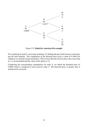
Long American Put To show how the value of an American put is computed, we use the
following parameters from Hull, page 247 [7], which is shown in5 Figure 2.5.
S0 = 50, K = 52, r = 0.05, u = 1.2, d = 0.8, ∆t = 1 and T = 2 years
The probability of an upward movement equals
p =
e0.05×1 −0.8
1.2−0.8
= 0.6282
Thus the probability of a downward movement is
(1− p) = 0.3718
The corresponding tree shows the price of the underlying asset at each node and the value of
the option at maturity. Recall that the pay-off for put options equals max{(K −St),0}.
We can see that holding the option to maturity could give a pay-off of either 0, 4 or 20. As
in the previous example we can not know how the underlying asset is priced at maturity, but
we know that we have the possibility to exercise the option early. Thus we work backwards
through the tree to evaluate the option price at each time step. Then we compare the binomial
value with the exercise value. The one that is greater tells how to proceed with the option. If
the binomial value is greater, we continue to hold the option. At t1 the option is either out of
the money (node B), or it generates a pay-off of 12. We should clearly not exercise if we end
up at B. Since the chance of a positive pay-off due to the end of the option is only 37.18%, the
value of the put is expected to be low. Calculation yields
e−0.05×1
(0.6282×0+0.3718×4) = 1.4147
The binomial value of 1.4147 is greater than the exercise value of zero. The option should
therefore be held.
5In the second rows we show the asset prices and in the third rows the payoffs.
26](https://image.slidesharecdn.com/056831bc-2170-4601-b463-4525efb79d14-150711133700-lva1-app6892/85/Bachelor-Thesis-Report-28-320.jpg)
![Chapter 3
Convergence of binomial model to
Geometric Brownian motion
3.1 Introduction and Background
As we saw in the previous section, in Cox, Ross and Rubinstein’s approach, if n → ∞, the
behavior of he binomial models can be approximated as a stochastic process in continuous
time. Black and Scholes 1973 [1] and Merton 1973 [15] assumed that the dynamic of a risky
security price follows a Geometric Brownian Motion. Following the Cox, Ross and Rubin-
stein’s approach it is possible to see that the sequence of the binomial models also converges
to a Geometric Brownian Motion [12],[14]. To begin with, we can express some definitions:
Definition 3.1.1. A stochastic process (Wiener Process) W(t), 0 ≤ t ≤ T, is called a standard
Brownian Motion if [12],[6],[14]
1. W(0) = 0.
2. W(t) is continuous on [0,T] with probability 1.
3. W(t) has independent increments.
4. the increment W(t)−W(s) is normally distributed with mean zero and variance t −s.
Theorem 3.1.1. Let W(t)−W(s) be a normal random variable. A Brownian Motion with drift
coefficient {µ,µ ∈ R} and σ > 0 coefficients is
G(t) = µt +σW(t)
Here µ and σ2 may be time-dependent. [12],[6],[14].
Definition 3.1.2. Let G(t) be a Brownian motion with drift coefficient µ and diffusion coeffi-
cient σ and S(0) be a positive real number. Then the process
S(t) = S(0)eG(t)
= S(0)eµt+σW(t)
(3.1)
28](https://image.slidesharecdn.com/056831bc-2170-4601-b463-4525efb79d14-150711133700-lva1-app6892/85/Bachelor-Thesis-Report-30-320.jpg)
![is called Geometric Brownian Motion [12],[6],[14].
From now on we denote X = ST /S0 and Y = ln(ST /S0). Moreover, Y is a random variable
which is normally distributed, and X is a random variable which is log-normally distributed.
Now we will continue with some investigations on different results for the binomial models.
Recalling (2.18) and (2.19) for the random variable X in a one-step binomial tree, we will
have1:
E[X] = E[ST /S0] = p∗
u+(1− p∗
)d
V[X] = V[(ST /S0)] = p∗
u2
+(1− p∗
)d2
−(E[X])2
Substituting the value of (E[X])2
and simplifying V[X] will yield:
V[X] = p∗
u2
+(1− p∗
)d2
−(p∗
u+(1− p∗
)d)2
= p∗
u2
+d2
− p∗
d2
− p∗2
u2
−2p∗
(1− p∗
)ud −(1− p∗
)2
d2
= p∗
u2
− p∗2
u2
+ p∗
d2
− p∗2
d2
−2p∗
ud +2p∗2
ud
= p∗
(1− p∗
)(u−d)2
To find the expected value and variance of the random variable Y we will do the following
steps. Firstly, we know that the possible stock prices at a one step binomial tree are:
ST =
S0u ,if stock goes up with probability p
S0d ,if stock goes down with probability 1-p
Since S0 is constant we can divide both hand sides with S0. Additionally, for obtaining random
variable Y we then can take the natural logarithm from both hand sides. Doing this will give
us:
Y = ln
ST
S0
=
lnu ,if stock goes up with probability p
lnd ,if stock goes down with probability 1-p
Finally, considering Definition 2.2.3 and calculating the expected value with (2.5) will give
us:
E[Y] = E [ln(ST /S0)] = p∗
lnu+(1− p∗
)lnd
Considering Theorem 2.2.2 and calculating the variance with (2.6) will yield:
V[Y] = V [ln(ST /S0)] = p∗
[lnu]2
+(1− p∗
)[lnd]2
−(E[Y])2
1A variable has log-normal distribution if the natural logarithm of the variable is normally distributed [7].
29](https://image.slidesharecdn.com/056831bc-2170-4601-b463-4525efb79d14-150711133700-lva1-app6892/85/Bachelor-Thesis-Report-31-320.jpg)
![Substituting the value of (E[Y])2
and simplifying V[Y] will yield:
V[Y] = p∗
[lnu]2
+(1− p∗
)[lnd]2
−[p∗
lnu+(1− p∗
)lnd]2
= p∗
(lnu)2
+(lnd)2
− p∗
(lnd)2
− p∗2
(lnu)2
−2p∗
(1− p∗
)lnulnd −(1− p∗
)2
(lnd)2
= p∗
(lnu)2
− p∗2
(lnu)2
+ p∗
(lnd)2
− p∗2
(lnd)2
−2p∗
lnulnd +2p∗2
lnulnd
= p∗
(1− p∗
) (lnu)2
−2lnulnd +(lnu)2
= p∗
(1− p∗
)[lnu−lnd]2
Remark 3.1.1. Now we have a system of equations for both normal and log-normal random
variables whit some unknown parameters p, u and d in a binomial lattice. We can remember
that Cox, Ross and Rubinstein also ended up with two equations for expected value and vari-
ance and three unknowns p, u and d. They solved this system of equations after calculating p
and they let ud = 1 to obtain an equal number of equations and unknowns.
Now let us consider the sequence of binomial models and its convergence to the Geometric
Brownian Motion.
3.2 The sequence of the binomial models and its conver-
gence to Geometric Brownian Motion
In this part we will investigate the sequence of the binomial models and its convergence to
Geometric Brownian Motion. To begin with, we can expand the sequence of the random
variable Y as follows [12],[14]:
E[Y] = E
t
∑
k=1
Yn,k = E ln
Sn,t
Sn,0
= E [Yn,1 +Yn,2 +...+Yn,t], 1 ≤ t ≤ n (3.2)
We have already calculated the expected value for Y, so the expected value at each time will
be:
E [Yn,t] = plnun +(1− p)lndn
We have already seen in the CRR model that as n → ∞ the expected value and variance of our
process µT and σ2T [4].
Moreover, we want the binomial model to converge to the Geometric Brownian Motion. So
we will have:
Y = µt +σW(t) 0 ≤ t ≤ T
E[Y] = µT V[Y] = σ2
T
Additionally, we know that in an n step binomial tree we have one random variable; let us call
it m, which can take a certain number of upward movements. Then the number of downward
movements will be n − m [4]. So the possible value for upward movements is un = um and
30](https://image.slidesharecdn.com/056831bc-2170-4601-b463-4525efb79d14-150711133700-lva1-app6892/85/Bachelor-Thesis-Report-32-320.jpg)
![the possible value for downward movements is dn = dn−m. For simplicity we will denote
xn = lnun and yn = lndn. Using the formulas for variance and expected value in the binomial
model we will have [4],[12],[14]
E[Y] = n[pxn +(1− p)yn] = µT
V[Y] = np(1− p)(xn −yn)2
= σ2
T
considering the fact that dn < un, we know that yn < xn. We can re-write the equation as
follows and solve the system of two equations with two unknowns.
pxn +(1− p)yn = µT/n
xn −yn = σ T
np(1−p)
Solving this system of equations will give:
xn = µT
n +σ 1−p
p
T
n
yn = µT
n −σ p
1−p
T
n
(3.3)
Recall (3.2). Since our sequence is a sequence of independent identically random variables,
we will have nE[Yn,1] = µT and nV[Yn,1] = σ2T. Now we can apply the central limit theorem
[12],[14]
lim
n→∞
P
Yn,1 +Yn,2 +...+Yn,n −nE[Yn,1]
nV[Yn,1]
≤ x = p
ln(ST /S0)− µT
σ
√
T
≤ x = Φ(x)
This proves that binomial models at time T, follow the normal distribution with mean µT and
σ2T.
3.3 The sequence of binomial models and its convergence to
Black-Scholes model under risk-neutral probability
We have already shown that binomial models at time T converge to the normal distribution
with mean µT and variance σ2T. Moreover, recall that Black and Scholes 1973 and Merton
1973 considered that the risky stock follows a Geometric Brownian Motion with drift coeffi-
cient µ and diffusion coefficient σ. Black and Scholes proved that in their model, risky stocks
are following the Geometric Brownian Motion with mean µ = r − σ2
2 T and variance σ2T
[1]. We will follow Black and Scholes approach and we will derive their pricing formula in the
appendix of this thesis. Since we are talking about pricing options via lattice approaches and
our random variable ST is discrete, we would like to investigate if pricing options using the
31](https://image.slidesharecdn.com/056831bc-2170-4601-b463-4525efb79d14-150711133700-lva1-app6892/85/Bachelor-Thesis-Report-33-320.jpg)
![binomial models converges to the Black-Scholes formula where ST is a continuous random
variable. So we will investigate the convergence of the binomial model to the Black-Scholes
model under risk neutral probability measure. First, for risk neutral probability measure we
have [12],[14]
p∗
n =
er T
n −dn
un −dn
, 1− p∗
n =
un −er T
n
un −dn
(3.4)
From (3.3) we can obtain 2:
xn = lnun ⇒ un = exn = exp µT
n +σ 1−p
p
T
n
yn = lndn ⇒ dn = eyn = exp µT
n −σ p
1−p
T
n
(3.5)
Substituting (3.5) in (3.4), we will obtain:
p∗
n =
er T
n −d
u−d
=
exp rT
n −exp µT
n −σ p
1−p
T
n
exp µT
n +σ 1−p
p
T
n −exp µT
n −σ p
1−p
T
n
=
exp (r − µ)T
n −exp −σ p
1−p
T
n
exp σ 1−p
p
T
n −exp −σ p
1−p
T
n
1− p∗
n =
u−er T
n
u−d
=
exp µT
n +σ 1−p
p
T
n −exp rT
n
exp µT
n +σ 1−p
p
T
n −exp µT
n −σ p
1−p
T
n
=
exp σ 1−p
p
T
n −exp (r − µ)T
n
exp σ 1−p
p
T
n −exp −σ p
1−p
T
n
It can be shown that limn→∞ p∗
n = p and limn→∞(1− p∗
n) = 1− p [12],[14].
Using the last result we can calculate the variance of binomial model as n → ∞ [12],[14]:
lim
n→∞
V∗
[Y] = lim
n→∞
np∗
(1− p∗
)(un −lndn)2
= lim
n→∞
np(1− p)(xn −yn)2
2Rendleman and Bartter 1979 got the same result in [16].
32](https://image.slidesharecdn.com/056831bc-2170-4601-b463-4525efb79d14-150711133700-lva1-app6892/85/Bachelor-Thesis-Report-34-320.jpg)
![Substituting xn and yn from (3.3) we will calculate [12],[14]:
lim
n→∞
V∗
[Y] = lim
n→∞
np(1− p)
µT
n
+σ
1− p
p
T
n
−
µT
n
−σ
p
1− p
T
n
2
= lim
n→∞
np(1− p) σ
T
n
1− p
p
+
p
1− p
2
= lim
n→∞
np(1− p)
σ2T
n
1− p
p
+2
1− p
p
×
p
1− p
+
p
1− p
= lim
n→∞
p(1− p)σ2
T
(1− p)2 + p2
p(1− p)
+2
= p(1− p)σ2
T
1
p(1− p)
−2
p(1− p)
p(1− p)
+2 = p(1− p)σ2
T
1
p(1− p)
= σ2
T
Secondly, for the expected value we have:
lim
n→∞
E∗
[Y] = lim
n→∞
n[p∗
xn +(1− p∗
)yn]
= lim
n→∞
n
exp (r − µ)T
n −exp −σ p
1−p
T
n
exp σ 1−p
p
T
n −exp −σ p
1−p
T
n
×
µT
n
+σ
1− p
p
T
n
+
exp σ 1−p
p
T
n −exp (r − µ)T
n
exp σ 1−p
p
T
n −exp −σ p
1−p
T
n
×
µT
n
−σ
p
1− p
T
n
= r −
σ2
2
T
To solve the last equation the Maclaurin expansion was used. Furthermore, applying the
central limit theorem we will obtain:
lim
n→∞
P∗ Y −nµn]
σn
√
n
≤ x = p∗ ln(ST /S0)−(r − σ2
2 )T
σ
√
T
≤ x = Φ(x)
which means, under risk-neutral probability measure, our stochastic process (binomial mod-
els) at time T converges to normal distribution with mean (r − σ2
2 )T and variance σ2T.
33](https://image.slidesharecdn.com/056831bc-2170-4601-b463-4525efb79d14-150711133700-lva1-app6892/85/Bachelor-Thesis-Report-35-320.jpg)
![3.4 Mean and variance of a random variable which is log-
normally distributed
As we have shown in the previous part, binomial models at time T converges to normal distri-
bution. In lots of scientific fields as well as finance, it is common to calculate and derive the
expectation and variance formulas for a random variable which is log-normally distributed. So
we will try to show how the expected value and variance of a random variable can be derived
from a normal distribution. To begin with we write some definitions [21].
Definition 3.4.1. A random variable U is said to have a normal probability distribution if and
only if, for σ > 0 and −∞ < µ < ∞, the density function of U is:
f(u) =
1
σ
√
2π
e−(u−µ)2/(2σ2)
, −∞ < u < ∞
and the following theorem tells us [21]:
Theorem 3.4.1. If U is a normally distributed random variable with parameter µ and σ, then:
E[U] = µ and V[U] = σ2
It is possible to transform a normal random variable U to a standard normal random variable
Z by [21]:
Z =
U − µ
σ
Applying Definition 3.4.1 and Theorem 3.4.1 to our random variable Y, we will have:
f(y) =
1
σ
√
2π
e−(y−µy)2/(2σ2
y )
, −∞ < y < ∞
where we have already calculated the mean and variance of binomial models at time T and its
convergence to normal distribution:
E[Y] = µy = µT and V[Y] = σ2
y = σ2
T
Now, we can continue with another definition [21]:
Definition 3.4.2. If a random variable Y is normally distributed with mean µy and variance
σ2
y and X = eY [equivalently, Y = lnX], then X is said to have a log-normal distribution.
Then the density function for X is:
f(x) =
1
xσ
√
2π
e−(lnx−µy)2/(2σ2
y )
, x > 0
0, elsewhere.
(3.6)
34](https://image.slidesharecdn.com/056831bc-2170-4601-b463-4525efb79d14-150711133700-lva1-app6892/85/Bachelor-Thesis-Report-36-320.jpg)
![Corollary 3.4.1. IfY is normally distributed with mean µy and variance σ2
y . Then the expected
value and variance of the log-normal distribution for a random variable X, where X = eY
[equivalently, Y = lnX], are given by
E[X] = e(µy+σ2/2)
and V[X] = (E[X])2
(eσ2
y −1)
Proof. We know that the expected value of a continuous random variable is:
E[X] =
∞
−∞
x f(x)dx
where f(x) is the density function of the random variable x. Substituting (3.6), we will get:
E[X] =
∞
−∞
x
1
xσy
√
2π
e−(lnx−µy)2/(2σ2
y )
dx
Now, we can use the property of the moment generating function and calculate E[eY ] instead
[21]. Then we will have x = ey ⇒ dx = eydy. Substituting we will obtain:
E[X] = E[eY
] =
∞
−∞
1
σy
√
2π
e−(y−µy)2/(2σ2
y )
(ey
dy)
Again, for simplicity we can change the variable z = y− µy ⇒ dz = dy and y = z+ µ ⇒ ey =
eµy+z. So the expected value will be:
E[X] = E[eY
] =
∞
−∞
eµy+z 1
σy
√
2π
e−z2/(2σ2
y )
dz = eµy
∞
−∞
1
σy
√
2π
ez−z2/(2σ2
y )
dz
Then we can do as follow:
z−z2
(2σ2
y )
= −
z
√
2σy
2
−z+
√
2σy
2
2
−
√
2σy
2
2
= −
z
√
2σy
−
√
2σy
2
2
−
σ2
y
2
= −
z−σ2
y
√
2σy
2
−
σ2
y
2
=
− z−σ2
y
2
2σ2
y
+
σ2
y
2
Now, let us denote w = z−σ2
y ⇒ dz = dw. Substituting w and dw, our integral will change
as follows:
E[X] = E[eY
] =
e(µy+σ2
y /2)
σy
√
2π
∞
−∞
e−w2/(2σ2
y )
dw
35](https://image.slidesharecdn.com/056831bc-2170-4601-b463-4525efb79d14-150711133700-lva1-app6892/85/Bachelor-Thesis-Report-37-320.jpg)
![Solving this integral is complicated, but we can use a typical trick and calculate the square
value of the expected value and then the positive square root of the result will be the answer.
So, we will have:
(E[X])2
= (E[eY
])2
=
e(2µy+σ2
y )
2πσ2
y
∞
−∞
∞
−∞
e−(v2+w2)/(2σ2
y )
dvdw
To solve this integral we can use polar form and change variables v = rcosθ, w = rsinθ,
dvdw = det(J)drdθ and det(J) = r. Where det(J) is the Jacobian . So we will have:
v2
+w2
= r2
cos2
θ +r2
sin2
θ = r2
(cos2
+sin2
) = r2
and the integral will be:
(E[X])2
= (E[eY
])2
=
e(2µy+σ2
y )
2πσ2
y
∞
0
2π
0
re−r2/(2σ2
y )
drdθ
=
e(2µy+σ2
y )
σ2
y
∞
0
re−r2/(2σ2
y )
dr
= −e(2µy+σ2
y )
∞
0
−2r
2σ2
y
e−r2/(2σ2
y )
dr
= −e(2µy+σ2
y )
e−r2/(2σ2
y )
∞
0
= −e(2µy+σ2
y )
(lim
r→∞
e−r2/(2σ2
y )
−e0
)
= −e(2µy+σ2
y )
(0−1) = e(2µy+σ2
y )
taking square root of the last result, will yield:
E[X] = E[eY
] = e(2µy+σ2
y )
1/2
= e(µy+σ2
y /2)
Substituting the value for σ2
y = σ2T and µy = µT, we will obtain the mean of the log-normal
distribution.
E[X] = e(µ+1
2 σ2)T
To calculate the variance we have:
V[X] = E[(X)2
]−(E[X])2
(3.7)
We have already known the result of (E[X])2. To calculate the E[X2] we can use the property
of the moment generating function [21] and we will have:
E[X2
] = E[e2Y
] =
∞
−∞
1
σy
√
2π
e−(y−µy)2/(2σ2
y )
(e2y
dy)
36](https://image.slidesharecdn.com/056831bc-2170-4601-b463-4525efb79d14-150711133700-lva1-app6892/85/Bachelor-Thesis-Report-38-320.jpg)
![Again, for simplicity we can change the variable u = y− µy ⇒ du = dy and y = u+µ ⇒ e2y =
e2(µy+z). So, the expected value will be:
E[X2
] = E[e2Y
] =
∞
−∞
e2(µy+u) 1
σy
√
2π
e−u2/(2σ2
y )
du
= e2µy
∞
−∞
1
σy
√
2π
e2u−u2/(2σ2
y )
du
= e2µy
∞
−∞
1
σy
√
2π
e
−(u2−4uσ2
y )
2σ2
y du
= e2µy
∞
−∞
1
σy
√
2π
e
−(u2−4uσ2
y +(2σ2
y )2−(2σ2
y )2
2σ2
y du
= e2(µy+σ2
y )
∞
−∞
1
σy
√
2π
e
−(u−2σ2
y )2
2σ2
y du
= e2(µy+σ2
y )
Substituting the value for E[X2] = e2(µy+σ2
y )
in (3.7), we will get:
V[X] = e2(µy+σ2
y )
−e(2µy+σ2
y )
= e2µy+σ2
y eσ2
y −1
And finally, substituting σ2
y = σ2T and µy = µT, we will get:
V[X] = e(2µ+σ2)T
eσ2T
−1
Remark 3.4.1. Calculating such integrals is usual for continuous random variables. So, hav-
ing proper skills to calculate ordinary and stochastic integrals is vital for a financial analyzer.
Remark 3.4.2. Often in literature we can see that the authors do not calculate the integ-
rals; they jumped to the results. Considering the calculation above we can explain it. As
we saw a density function for a normal random variable X ∼ N[µ,σ] is given by φ(x) =
1
σ
√
2π
e−(x−µ)2/2σ2
, then considering the calculations above, we know that the distribution
function of a normal random variable has the value of Φ(X) = X
−∞ φ(x)dx. As an example,
for a standard normal random variable Z, where µ = 0 and variance is σ = 1 or equival-
ently Z ∼ N[0,1], we can directly say that the density function of a standard normal random
variable Z is φ(z) = 1√
2π
e−z2/2 and Φ(Z) = Z
−∞ φ(z)dz. So, if we can make the form of our
integral like an integral of a density function for the standard normal random variable, then
we can find the probability (area under normal curve) from the standard normal probability
table. Additionally, if we have a normal random variable instead of standard normal variable,
we can transform the normal variable to standard normal random variable and again use the
table to find the probability. Finally, it is easy to say the area under the any density function is
one or equivalently ∞
−∞ φ(z)dz = 1 [21].
37](https://image.slidesharecdn.com/056831bc-2170-4601-b463-4525efb79d14-150711133700-lva1-app6892/85/Bachelor-Thesis-Report-39-320.jpg)
![Chapter 4
Different approaches on Binomial
Models
In the previous chapter we calculated the expected value and variance of the normal and log-
normal distribution for normal and log-normal random variables. Then we calculated the ex-
pected value and variance of the binomial models which converges to a Geometric Brownian
Motion. Moreover, we have seen that the sequence of binomial models at time T converges
to the Geometric Brownian Motion under risk-neutral probability. So if we want to estim-
ate binomial models with Log-normal distribution and at the same time we want that our
model converges to a Geometric Brownian Motion, we can substitute the expected value1
µy = r − σ2
2 T and variance σ2
y = σ2T of the Geometric Brownian Motion to our expected
value and variance formulas which we have obtained for log-normal distribution [17]. Thus
we will have:
lim
n→∞
E∗
[X] = lim
n→∞
n[pu+(1− p)d]
= e(µy+1
2 σ2
y )
= e(r−1
2 σ2+1
2 σ2)T
= erT
lim
n→∞
V∗
[X] = lim
n→∞
np(1− p)(u−d)2
= e(2µy+σ2
y )
eσ2
y −1 = e(2r−σ2+σ2)T
eσ2T
−1
lim
n→∞
V∗
[X] = e2rT
eσ2T
−1
X ∼ LN rT,σ2
T
Again, we will have two equations for expected value and variance and three unknowns u, d
and p. We can choose different value for either p, u or d to obtain our third equation and make
a survey of different binomial models where we want results to converge to the Geometric
1We know that in risk neutral probability measure, or equivalent Martingale probability measure, the drift
coefficient is equal to the risk-free interest rate.
38](https://image.slidesharecdn.com/056831bc-2170-4601-b463-4525efb79d14-150711133700-lva1-app6892/85/Bachelor-Thesis-Report-40-320.jpg)
![Brownian Motion [17]. Additionally, our calculation was for n step binomial models. Con-
sidering this fact, we can say that in each step we will have ∆t = T/n, and we can calculate
the expected value and variance for each step in the binomial tree. So for X = Si+1
Si
which is
log-normally distributed we will have [17]:
X =
Si+1
Si
E[X] = pu+(1− p)d = er∆t
V[X] = p(1− p)(u−d)2
= e2r∆t
eσ2∆t
−1
X ∼ LN r∆t,σ2
∆t
For Y = ln Si+1
Si
which is normally distributed, we will have:
Y = ln
Si+1
Si
E[Y] = plnu+(1− p)lnd = (r −
σ2
2
)∆t
V[Y] = p(1− p)[lnu−lnd]2
= σ2
∆t
Y ∼ N (r −
σ2
2
∆t,σ2
∆t
Now we have the system of two equations for both normal and log-normal random variables
whit three unknown parameters p, u and d in a binomial lattice. IN next two sections we will
introduce the third equation when the stock price is normally and log-normally distributed by
p = 1/2 and ud = 1 and we will try to calculate p, u and d. Then we will make a survey on
some well-known and famous binomial models2[17].
4.1 Random variableY = ln
Si+1
Si
is normally distributed
When the random variable Y = ln Si+1
Si
is normally distributed, we will have two equations
for expected value and variance and three unknowns p, u and d. Here we will introduce one
extra equation to increase our equations to three and then we will solve a system of three
equations and three unknowns.
2We had already written a preliminary version of our thesis when we found an interesting paper "Two-State
Option Pricing: Binomial Models Revisited" by Jabbour, Kramin and Young [8]. We would suggest that the
reader looks at that paper as well.
39](https://image.slidesharecdn.com/056831bc-2170-4601-b463-4525efb79d14-150711133700-lva1-app6892/85/Bachelor-Thesis-Report-41-320.jpg)
![4.1.1 Introducing the third equation by p = 1/2
Writing the equations for the expected value and variance of the random variable Y, which is
normally distributed, we will have two equations and three unknowns:
E[Y] = plnu+(1− p)lnd = (r −
σ2
2
)∆t
V[Y] = p(1− p)[lnu−lnd]2
= σ2
∆t
Substituting p = 1/2 we will get the system of two equations with two unknowns.
(lnu−lnd)2 = 4σ2∆t
lnu+lnd = (2r −σ2)∆t
We denote x = lnu and y = lnd. Moreover, since u > d ⇒ x > y, we will have:
x−y = 2σ
√
∆t
x+y = (2r −σ2)∆t
we will obtain:
x = (r −
σ2
2
)∆t +σ
√
∆t ⇒ u = e(r−σ2
2 )∆t+σ
√
∆t
y = (r −
σ2
2
)∆t −σ
√
∆t ⇒ d = e(r−σ2
2 )∆t−σ
√
∆t
Remark 4.1.1. The value for p is different in the Jarrow-Rudd model, but as we will see later,
the values for the u and d factors in our approach are exactly the same as the values for u
and d factors which have been derived by Jarrow and Rudd. However, Jarrow and Rudd have
shown that p = 1/2 as ∆t → 0 [10],[9].
Remark 4.1.2. We can consider the formula which was obtained by Rendleman and Bartter
[16], which is as follows
u = exp µT
n +σ 1−p
p
T
n
d = exp µT
n −σ p
1−p
T
n
Where p is unknown. Susbtituting p = 1/2 we will obtain exactly the same result for u and d
in our calculations.
Remark 4.1.3. In this model ud = e(2r−σ2)∆t, whereas in the CRR model ud = 1.
4.1.2 Introducing the third equation by ud = 1
Again, we have two equations and three unknowns.
E[Y] = plnu+(1− p)lnd = (r −
σ2
2
)∆t
V[Y] = p(1− p)[lnu−lnd]2
= σ2
∆t
40](https://image.slidesharecdn.com/056831bc-2170-4601-b463-4525efb79d14-150711133700-lva1-app6892/85/Bachelor-Thesis-Report-42-320.jpg)
![Substituting d = 1/u we will get a system of two equations with two unknowns.
p(1− p)(lnu−lnu−1)2 = p(1− p)(lnu+lnu)2 = σ2∆t
plnu+(1− p)lnu−1 = plnu−(1− p)lnu = (r − σ2
2 )∆t
We denote x = lnu and y = lnd. Moreover, since u > d ⇒ x > y, we will have:
4p(1− p)x2 = σ2∆t
px−(1− p)x = x[p−(1− p)] = (r − σ2
2 )∆t
we will obtain:
x =
(r − σ2
2 )∆t
2p−1
p− p2
=
σ2∆t
4x2
Substituting and denoting a = (r − σ2
2 )2∆t we can solve the equations above for p:
p2
− p+
σ2∆t
4
(r−σ2
2 )∆t
2p−1
2
= 0
p2
− p+
σ2(4p2 −4p+1)
4(r − σ2
2 )2∆t
= 0 ⇒ ap2
−ap+σ2
p2
−σ2
p+
σ2
4
= 0
p2
(a+σ2
)− p(a+σ2
)+σ2
= 0
p2
− p+
σ2
4(a+σ2)
= 0
then
p1,2 =
1± (−1)2 −4σ2/4(a+σ2)
2
p =
1
2
±
1
2
×
a+σ2 −σ2
a+σ2
=
1
2
+
1
2
×
√
a
√
a+σ2
p1,2 =
1
2
±
1
2
×
√
∆t(r − σ2
2 )
√
∆t σ2
∆t +(r − σ2
2 )2
p=
1
2
+
1
2
×
(r − σ2
2 )
σ2
∆t +(r − σ2
2 )2
41](https://image.slidesharecdn.com/056831bc-2170-4601-b463-4525efb79d14-150711133700-lva1-app6892/85/Bachelor-Thesis-Report-43-320.jpg)
![To calculate x we can use the variance formula which is much more convenient and will help
us to avoid the quadratic calculation.
V[Y] = p[ln(u)]2
+(1− p)[ln(d)]2
−(E[Y])2
= σ2
∆t
p[ln(u)]2
+(1− p)[ln(d)]2
− (r −
σ2
2
)∆t
2
= σ2
∆t
p[ln(u)]2
+(1− p)[ln(u−1
)]2
− (r −
σ2
2
)∆t
2
= σ2
∆t
p[ln(u)]2
+(1− p)[−ln(u)]2
− (r −
σ2
2
)∆t
2
= σ2
∆t
px2
+(1− p)(−x)2
− (r −
σ2
2
)∆t
2
= σ2
∆t
x = σ2∆t + (r −
σ2
2
)∆t
2
u = e
σ2∆t+ (r−σ2
2 )∆t
2
d = e
− σ2∆t+ (r−σ2
2 )∆t
2
Remark 4.1.4. Our calculation to derive p raise a controversial question. Can we obtain
two answers for p which both lie between zero and one? Perhaps yes. Because, the term
1
2 ×
(r−σ2
2 )
σ2
∆t +(r−σ2
2 )2
must lie between −1/2 and 1/2, since, the probability p must lie between
zero and one. So perhaps we can say:
p1,2 = 1
2 ± 1
2 ×
(r−σ2
2 )
σ2
∆t +(r−σ2
2 )2
So, if we choose a negative sign, then p can be close to zero and if we choose a plus sign, p
can be close to one, which is what we expected.
Remark 4.1.5. In this model we have the same arguments as in all binomial models which we
have considered. If n → ∞ then ∆t → 0 then limn→∞ pn = 1/2.
42](https://image.slidesharecdn.com/056831bc-2170-4601-b463-4525efb79d14-150711133700-lva1-app6892/85/Bachelor-Thesis-Report-44-320.jpg)
![4.2 Random variable X =
Si+1
Si
is log-normally distributed
When the random variable X = Si+1
Si
is log-normally distributed, we will have two equations for
expected value and variance and three unknowns p, u and d. Here we will introduce one extra
equation to increase our equations to three and then we will solve a system of three equations
and three unknowns.
4.2.1 Introducing the third equation by p = 1/2
Writing a system of two equations and three unknowns, we will have:
E[X] = pu+(1− p)d = er∆t
V[X] = p(1− p)(u−d)2
= e2r∆t
eσ2∆t
−1
Substituting p = 1/2 we will obtain:
u+d = 2er∆t
⇒ u = 2er∆t
−d
(u−d)2
= 4e2r∆t
eσ2∆t
−1
substituting u:
(2er∆t
−d −d)2
= (2er∆t
−2d)2
= (4e2r∆t
−8der∆t
+4d2
) = 4e2r∆t
eσ2∆t
−1
⇒d2
−2er∆t
d −e2r∆t
eσ2∆t
−2 = 0
d1,2 =
2er∆t ± (−2er∆t)2 +4e2r∆t eσ2∆t −2
2
d1,2 = er∆t
± e2r∆t +e2r∆t eσ2∆t −2
d1,2 = er∆t
±er∆t
eσ2∆t −1
since d < u then:
u = er∆t
1+ eσ2∆t −1
d = er∆t
1− eσ2∆t −1
43](https://image.slidesharecdn.com/056831bc-2170-4601-b463-4525efb79d14-150711133700-lva1-app6892/85/Bachelor-Thesis-Report-45-320.jpg)
![Remark 4.2.1. In this model, we will have:
ud = e2r∆t
12
− eσ2∆t −1
2
= e2r∆t
2−eσ2∆t
4.2.2 Introducing the third equation by ud = 1
Solving the following equation for p we will have:
E[X] = pu+(1− p)d = er∆t
⇒ pu+d − pd = p(u−d)+d = er∆t
⇒ p =
er∆t −d
u−d
=
uer∆t −1
u2 −1
and solving the variance equation for u we will get:
V[X] = p(1− p)(u−d)2
= e2r∆t
eσ2∆t
−1
⇒
uer∆t −1
u2 −1
×
u(u−er∆t)
u2 −1
×
u2 −1
u
2
= e2r∆t
eσ2∆t
−1
⇒
u2er∆t −ue2r∆t −u+er∆t
u
= e2r∆t
eσ2∆t
−1
⇒ u2
er∆t
−ue2r∆t
−u+er∆t
−ue2r∆t
eσ2∆t
−1 = 0
⇒ u2
er∆t
−u e(2r+σ2
2 )∆t
+1 +er∆t
= 0
⇒ u1,2 =
e(2r+σ2
2 )∆t +1 ± e(2r+σ2
2 )∆t +1
2
−4e2r∆t
2er∆t
u =
1
2
e−r∆t
e(2r+σ2)∆t
+1 +
1
4
e−2r∆t e(2r+σ2)∆t +1
2
−1
d =
1
2
e−r∆t
e(2r+σ2)∆t
+1 −
1
4
e−2r∆t e(2r+σ2)∆t +1
2
−1
Remark 4.2.2. As we can see in this model, the value of p is equal to the risk-neutral prob-
ability measure in the CRR model, but the u and d factors are different. The reason is, in our
equation for variance we have a different value compared to the CRR model because from the
beginning, we constructed our model in such a way that our binomial model converges to the
Geometric Brownian Motion.
44](https://image.slidesharecdn.com/056831bc-2170-4601-b463-4525efb79d14-150711133700-lva1-app6892/85/Bachelor-Thesis-Report-46-320.jpg)
![4.3 The Jarrow-Rudd model
This model was proposed by Jarrow and Rudd [10]. However, we used additional literature
to study this model [9],[17]. We have already calculated the expected value and variance
of a random variable which is log-normally distributed. Using the previous result we have
[9]:
E[X] = E
ST
S0
= exp µT +
σ2
2
T
Since S0 is constant, the equation above can be rewritten as:
E[ST ] = S0 exp µT +
σ2
2
T
Moreover, we know that the option pricing follows a martingale process. Thus under the
equivalent martingale probability measure we have [9]:
Ep∗
[ST |S0] = S0 exp ˆµT +
σ2
2
T (4.1)
and considering the fact that in the risk-neutral world the expected return on a stock must be
equal to the risk-free interest rate, we can write the next equation as follows [9]:
S0 = e−rT
Ep∗
[ST |S0] (4.2)
Substituting (4.1) into (4.2) we will obtain ˆµ = r − σ2
2 , which means in the risk-neutral world
that the drift coefficient must be equal to r − σ2
2 .
Now we can approximate this process in the discrete binomial model. It follows [9]:
St+1 = St
u = e(r−σ2
2 )∆t+σ
√
∆t with probability p∗
d = e(r−σ2
2 )∆t−σ
√
∆t with probability 1− p∗
where p∗ = erT −d
u−d , and Y = St+1
St
∼ N (r − σ2
2 ∆t,σ2∆t . If we substitute the value of u and
d in our probability equation we will obtain [9]:
p∗
=
e
σ2
2 ∆t −e−σ
√
∆t
eσ
√
∆t −e−σ
√
∆t
Moreover, if we calculate the limit, we will obtain [9]:
lim
∆t→0
p∗
= lim
∆t→0
e
σ2
2 ∆t −e−σ
√
∆t
eσ
√
∆t −e−σ
√
∆t
=
1
2
Remark 4.3.1. As we can see, Jarrow and Rudd used a significantly different approach from
Black and Scholes. However, they find the same result for the drift and diffusion coefficient
under risk-neutral probability measure.
Remark 4.3.2. In the Jarrow-Rudd model ud = e(2r−σ2)∆t, whereas in the CRR model ud = 1.
45](https://image.slidesharecdn.com/056831bc-2170-4601-b463-4525efb79d14-150711133700-lva1-app6892/85/Bachelor-Thesis-Report-47-320.jpg)
![4.4 The Tian model
Tian introduce his binomial model in discrete time with following p, u and d factors:
p =
M −d
u−d
, q = 1− p =
u−M
u−d
u =
MV
2
V +1+ V2 +2V +3
d =
MV
2
V +1− V2 +2V +3
Now, let’s see how he derived equations above and what M and V stand for.
Tian constructed his model assuming that in a risk neutral world, the stock price is following
a stochastic process which is given by following the stochastic differential equation [19]:
dS(t)
S(t)
= rdt +σdW
Then he considered the logarithmic transformation of the process above. To do so, we de-
note F = ln(S(t)) and then we will apply Itô’s formula to the SDE above, so we will have
[19]:
dF =
∂F
∂t
dt +
∂F
∂S
dS+
1
2
∂2F
∂S2
(dS)2
dF = 0+
1
S
dS−
1
2S2
(dS)2
dF =
1
S
(rSdt +σSdW)−
1
2S2
σ2
S2
(dW)2
dF = (rdt +σdW)−
1
2
σ2
dt
dF = r −
σ2
2
dt +σdW
d lnS(t) = r −
σ2
2
dt +σdW (4.3)
Notice that (dW)2 = dt and (dt)2 = dtdW = 0. Considering (4.3) and the discussion we
had before, it is obvious that in (4.3) the one dimensional distribution is following a normal
distribution with mean (r − σ2
2 )t and variance σ2t. Thus the mth non-central moment of the
stock price can be interpreted by [19]:
E[S(t)m
|S0] = Sm
0 exp mr +(m−1)
σ2
2
t
46](https://image.slidesharecdn.com/056831bc-2170-4601-b463-4525efb79d14-150711133700-lva1-app6892/85/Bachelor-Thesis-Report-48-320.jpg)
![This is a formula for a stochastic process in continuous time. To approximate this formula in
discrete time with an n-step binomial model, we can say that ∆t = T
n . We assumed that the
price of a stock follows a binomial process which sometimes is called a two-jump process3.
Now, as we have discussed before, we want our binomial model to converge to the log-normal
distribution in continuous time. So, we have to choose the parameters u, d, p and q in a way
that guarantees our objective. Using our knowledge and the proofs we did before, we know
that in the binomial models, our random variable Y, is normally distributed. Moreover, us-
ing the result for the transformation of random variable X which is log-normally distributed,
we can express the expected value and variance of binomial models at time T when our ran-
dom variable is log-normally distributed. Thus we can write the following three equations
[19]:
p+q = 1
pu+qd = er∆t
= M
pu2
+qd2
= e(2r+σ2)∆t
= M2
V
Tian denotes M = er∆t and V = eσ2∆t. Substituting q = 1− p we have two equations and three
unknowns. Cox, Ross and Rubinstein considered a recombining tree with u = 1/d, but Tian
considered that the third moments of the discrete time process is also correct according to a
continuous time process, so he obtained the forth equation [19]:
pu3
+(1− p)d3
= M3
V3
Solving this system of equations, Tian got [19]:
p =
M −d
u−d
, q = 1− p =
u−M
u−d
u =
MV
2
V +1+ V2 +2V +3
d =
MV
2
V +1− V2 +2V +3
Remark 4.4.1. By comparing and contrasting the CCR model and the Tian model, we can say
that in the CRR model the variance is correct in the limit case and when ∆t → 0, whereas in
the Tian model, both mean and variance are true for any given ∆t [19].
Remark 4.4.2. Tian chose the correct third moment, but CCR chose ud = 1 for simplicity. In
the Tian model we have ud = (MV)2 [19].
3See [19]
47](https://image.slidesharecdn.com/056831bc-2170-4601-b463-4525efb79d14-150711133700-lva1-app6892/85/Bachelor-Thesis-Report-49-320.jpg)
![4.5 The Trigeorgis model
Trigeorgis began with the design of the log-transformed binomial model. Again, he considered
the diffusion process as follows [20]:
dS(t)
S(t)
= αdt +σdW
where α is expected value, σ is standard deviation and W is a Wiener process. Moreover,
X(t) ≡ lnS(t) follows Brownian motion. So under risk-neutral probability we will have α = r
and our process when, S(t) is log-normally distributed, will be [20]:
dX = ln
S(t +dt)
S(t)
= r −
σ2
2
dt +σdW
Again, in this process, ln S(t+dt)
S(t) or equivalently dX is normally distributed. So, we have
[20]:
E[dX] = r −
σ2
2
dt, V[dX] = σ2
dt
In order to approximate our continuous process in discrete time in each sub-interval ∆t = T/n,
X will follow a Markov random walk which with risk-neutral probability p goes up by the
amount ∆X = H ≡ u and with risk-neutral probability 1 − p goes down by the amount of
∆X = −H ≡ d [20]. It is easy to see that this binomial model is recombining. Thus calculating
the expected value and variance for this Markov process we will obtain [20]
E[∆X] = pH +(1− p)(−H) = 2pH −H ≡ pu+(1− p)d
V[∆X] = p(1− p)(2H)2
= 4pH2
−4p2
H2
≡ p(1− p)(u−d)
V[∆X] = H2
−(H2
−4pH2
+4p2
H2
) = H2
−(2pH −H)2
= H2
−(E[∆X])2
We will obtain a system of two equations with two unknowns [20]:
2pH −H = 2p∆X −∆X = ∆X(2p−1) = r −
σ2
2
∆t
4pH2
−4p2
H2
= 4p(∆X)2
(1− p) = σ2
∆t
Solving the equations we will obtain [20]:
∆X = σ2∆t + r −
σ2
2
2
(∆t)2
p =
1
2
1+ r −
σ2
2
∆t
∆X
Remark 4.5.1. It is easy to see that lim∆t→0 p = 1/2 in Trigeorgis model as well.
48](https://image.slidesharecdn.com/056831bc-2170-4601-b463-4525efb79d14-150711133700-lva1-app6892/85/Bachelor-Thesis-Report-50-320.jpg)
![4.6 The Leisen-Reimer model
One of the latest binomial models was proposed by Leisen and Reimer in 1996 [13],[17]. They
considered the Black-Scholes formula and the convergence of different binomial models to the
Black-Scholes formula. Leisen and Reimer proposed and proved a theorem about the order of
convergence in different binomial models. They showed that the previous models in discrete
time such as CCR, JR, Tian and more, have convergence to the Black and Scholes results with
order one. Their model however, has a second order of convergence (quadratic convergence)
[13]. To begin with, we write the Black-Scholes formula 4:
c(t,S0) = S0N(d1)−Ke−r(T−t)
N(d2), d1,2 =
ln(S0/K)+(r ± σ2
2 )(T −t)
σ
√
T −t
and the CRR option pricing formula5 [4]:
cn(tn
0 = 0,S0) = S0Φ(a;n, pn)−Kr−n
n Φ(a;n, pn)
where [13],[4]:
pn =
rn −dn
un −dn
pn = pn
un
rn
a =
ln(K/S0)−nlndn
lnun −lndn
Then they consider the fact that in all approaches which they have followed in the binomial
model, the probability p is approximated with the standard normal function N(z), where the all
input arguments are determined by some adjustment function z = h(a;n, p) [13]. Leisen and
Reimer denoted 6 a as the number of upward movements of the asset price to exceed strike
price in a n step binomial tree (lattice) with martingale probability measure p [13] instead.
Then they made an inverse transformation of the adjustment function where h(a;n, p) specifies
the distribution parameter h−1(z) = p to approximate P = N(z) with P ≈ 1−Φ(a;n, p) [13].
Then they used the Peizer and Pratt derivation of the inversion formula to the Camp-Paulson
method, one with7 [case : a+1/2 = n−(a+1/2),n = 2a+1] [13]:
h−1
(z) =
1
2
1
4
−
1
4
exp −
z
n+ 1
3
2
n+
1
6
1/2
After introducing the discussion above, Leisen and Reimer solved the system of equations
in such way which guarantees the convergence of the binomial model. In other words, they
needed to derive un, dn and pn. After a little algebra they obtained their new binomial model
with the following parameters [13]:
pn = h−1
(d1) pn = h−1
(d2)
un = rn
pn
pn
dn =
rn − pnun
1− pn
4To see the derivation of Black-Scholes option pricing formula, see Appendix A.
5To see the derivation see [4].
6This condition in the CRR model is given by a ≡ smallest non-negative integer greater than ln(K/S0)−nlndn
lnun−lndn
.
7Two see the result for Camp-Paulson inversion and Peizer-Pratt method two, see [13].
49](https://image.slidesharecdn.com/056831bc-2170-4601-b463-4525efb79d14-150711133700-lva1-app6892/85/Bachelor-Thesis-Report-51-320.jpg)
![Remark 4.6.1. By having the parameter Z in the Leisen-Reimer model, we can get a unique
distribution parameter p for each pair of (a,n). Thus in the continuous model the parameter
a(n) can be chosen freely, whereas in the discrete case a(n) and a (n) can be chosen freely but
they must be equal to determine pn and p (n) in the system of equations above [13].
Remark 4.6.2. With inverse transformation, we have to have an odd number of steps in this
model [13].
50](https://image.slidesharecdn.com/056831bc-2170-4601-b463-4525efb79d14-150711133700-lva1-app6892/85/Bachelor-Thesis-Report-52-320.jpg)
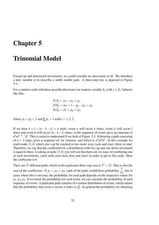
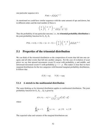
![E(Xi) = npi, V(Xi) = npiqi
Trinomial and multinomial models are an extension of binomial models. There are more
parameters involved, but the approach is the same, hence the similarity in the formulas. In
fact, the binomial model is a special case of multinomial models. The easiest way to see
that is to think about the marginal distribution. If we have two probabilities, we have two
scenarios with their corresponding events; if we have three probabilities, we have one scenario
with its corresponding event, and another scenario where this event not occurs. If we have n
probabilities, we can again say that we have two scenarios; one with its event and another one
where the first one not occurs (but all the others). This is well explained in Wackerly, et al,
pages 278 and 279 [21] which is the basic material used up to now in this section. There are
more explanations within the statements compared to the binomial model because it might be
a little bit harder to cope with the formulas when a third variable is involved.
(0,0)
S0
(1,2)
S0u
(1,1)
S0
(1,0)
S0d
(2,4)
S0u2
(2,3)
S0u
(2,2)
S0
(2,1)
S0d
(2,0)
S0d2
(3,6)
S0u3
(3,5)
S0u2
(3,4)
S0u
(3,3)
S0
(3,2)
S0d
(3,1)
S0d2
(3,0)
S0d3
Figure 5.1: Three-step trinomial tree
5.2 Boyle’s approach of deriving probabilities
In his paper [2], Boyle derived the values for the three probabilities and the values for u and
d implying that the log normal continuous distribution of the evolution of the stock price
53](https://image.slidesharecdn.com/056831bc-2170-4601-b463-4525efb79d14-150711133700-lva1-app6892/85/Bachelor-Thesis-Report-55-320.jpg)
![has the same properties as the discrete distribution, i.e., mean and variance of the respective
distributions equal each other. As we have seen before, the probabilities for the movements
sum up to 1. Therefore it is valid to substitute p2 by 1 − p1 − p3. In the continuation of the
explanation of this approach we use the same notation as Boyle which is
Su, S and Sd = price of the underlying asset after an upward, downward or horizontal move-
ment respectively,
r = interest rate, continuously compounded,
σ2 = variance of return,
h = length of one time interval, d =
1
u
.
The equation regarding equality between discrete and log normal continuous expected value
is
SM = Serh
SM = p1Su +(1− p1 − p3)S+ p3Sd
We rewrite this and obtain
p1(u−1)+ p3
1
u
−1 = M −1 (5.1)
The equation regarding equality between discrete and log normal continuous expected value
is
S2
V = S2
V = S2
M2
exp[(σ2
h)−1)]
S2
V = p1(S2
u2
−S2
M2
)+(1− p1 − p3)(S2
−S2
M2
)+ p3(
S2
u2
−S2
M2
)
which in rewritten form gives
p1(u2
−1)+ p3
1
u2
−1 = V +M2
−1. (5.2)
Now we solve (5.1) and (5.2) for p1 and p3.
The result is:
p1 =
(V +M2 −M)u−(M −1)
(u−1)(u2 −1)
54](https://image.slidesharecdn.com/056831bc-2170-4601-b463-4525efb79d14-150711133700-lva1-app6892/85/Bachelor-Thesis-Report-56-320.jpg)
![and
p3 =
(V +M2 −M)u2 −u3(M −1)
(u−1)(u2 −1)
p2 = 1− p1 − p3
What we can see directly from the equations is that u cannot attain the value 1 because it
would lead to zeros in the denominators. This is totally in line with the nature of an upward
movement. The factor has to be larger than one in order to make the value of the underlying
asset grow. Moreover, since we have two constraints and are looking for five unknowns u,
d, m, p1 and p3, we cannot find unique values for p1 and p3. Boyle used the Cox, Ross,
Rubinstein value u = eσ
√
∆t in the calculations in his paper, but pointed out that this could give
negative values for p2. Therefore he found it reasonable to slightly modify the expression by
including the variable λ so that
u = λeσ
√
∆t
where λ > 1, called stretch parameter.
Since it is not essential yet space consuming to show the actual calculations for p1 and p3, we
will not do them here. The Boyle paper is in our opinion a reliable and well known source, so
the result is trustworthy. For interested readers however, the authors of this thesis will provide
the calculations.
5.3 The replicating portfolio in the trinomial model
To show that there is no unique risk neutral probability measure, we studied the lecture notes
from lecture 5 of Stochastic processes by Anatoliy Malyarenko [14]. We changed the notation
for the value of the option C to f because it is more suitable for the linearity of our paper.
A replicating portfolio is a portfolio that has the same value as the derivative for the underlying
asset, independent of the price of the underlying.
For one single period the probabilities of the price change of an asset are as follows:
P{S(1) = uS} = p
P{S(1) = mS} = q
P{S(1) = dS} = 1− p−q
where p and q = (1 − p) are real numbers which are greater than zero and their sum is less
than one. Additionally d < m < u. Also, R = r +1 and lies between d and u.
The value of the portfolio after one ∆t is
55](https://image.slidesharecdn.com/056831bc-2170-4601-b463-4525efb79d14-150711133700-lva1-app6892/85/Bachelor-Thesis-Report-57-320.jpg)
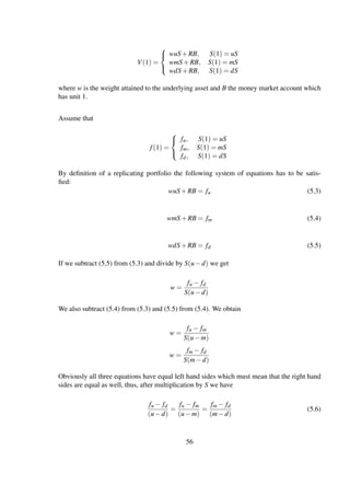
![If the condition described in the last equation is fulfilled, the contingent claim is attainable.
If this really is so, the simultaneous equations for fu, fm and fd give us the values for the
respective weights as
w =
fu − fm
S(u−m)
B =
ufm −mfu
R(u−m)
We already know from the Asset Pricing Theorem (Kijima page 87 [12]) that the fair price of
our option should be
f =
fu − fm
(u−m)
+
ufm −mfu
R(u−m)
If there are no arbitrage opportunities, we have a risk neutral probability measure P∗ such
that
P∗
{S(1) = uS} = p∗
P∗
{S(1) = mS} = q∗
P∗
{S(1) = dS} = 1− p∗
−q∗
For the underlying asset price to be a martingale under P∗ requires that
(u−d)p∗
+(m−d)q∗
= R−d
Similarly for the value of the contingent claim to be a martingale under P∗ is
(fu − fd)p∗
+(fm − fd)q∗
= fR− fd
The fair price of an option is
f = R−1
[p∗
fu +q∗
fm +(1− p∗
−q∗
)fd]
=
fu − fm
u−m
+
ufm −mfu
R(u−m)
+
m−d
u−m
(fu − fm)−(fm − fd) q∗
The very last term of the last equation vanishes if condition (5.6) holds.
There is no unique probability distribution (p∗, q∗, 1− p∗ −q∗) that satisfies the above equa-
tion, thus the market is incomplete because not every contingent claim is attainable.
57](https://image.slidesharecdn.com/056831bc-2170-4601-b463-4525efb79d14-150711133700-lva1-app6892/85/Bachelor-Thesis-Report-59-320.jpg)
![5.4 Trinomial probability under lognormal transformation
The Kamrad and Ritchken paper [11] explained this topic very well, so we used it as basic
material for this section.
For an underlying asset that follows a Geometric Brownian Motion we have parameters r,
riskless interest rate, and σ, instantaneous volatility (standard deviation), and drift
µ = r −
σ2
2
.
Since we want to calculate returns implementing continuous compounding, we would like to
explore the natural logarithm of the return over one time interval as
ln{S(t +∆t)} = ln{S(t)}+ζ(t)
This tells us that we can express our return as a sum consisting of two components: the log-
arithm of the price of the underlying at time t, and a random part ζ(t). The latter is a normal
random variable with mean µ∆t and variance σ2∆t.
Let ζa(t) be the approximating function over the interval [t,t +∆t] which is distributed in the
following way:
ζ(t) =
v with p1
0 with p2
−v with p3
3
∑
i=1
pi = 1
Notice that Kamrad and Ritchken were interested in the logarithm of S and emphasized it by
the use of v as variable for an upward movement (in contrast to u which we have seen earlier)
and we follow this approach. −v is of course a downward movement. Since u = eσ
√
∆t we set
v = λσ
√
∆t. The λ is needed in order to assure that p2 does not attain negative values, which
was suggested in Boyle [2].
The approximating distribution should have the same mean and variance as the random vari-
able ζ(t) so we can set the two formulas
E [ζa
(t)] = vp1 +0p2 +(−v)p3 = v(p1 − p3) = µ∆(t) (5.7)
and
58](https://image.slidesharecdn.com/056831bc-2170-4601-b463-4525efb79d14-150711133700-lva1-app6892/85/Bachelor-Thesis-Report-60-320.jpg)
![V [ζa
(t)] = v2
p1 +02
p2 +(−v2
)p3 = v2(p1 + p3 = σ2
∆t +o(∆t) (5.8)
o(∆t) stands for terms of higher order of ∆t which can be ignored if ∆t is very small.
For (5.7) we obtain
p1 =
µ∆t +vp3
v
which we plug into (5.8) so that we obtain
v2µ∆t +v3 p3
v
+v2
p3 = σ2
∆t
Solving for p3 and substituting v with λσ
√
∆t yields
p3 =
σ2∆t
2λ2σ2∆t
−
λσ
√
∆tµ∆t
2λ2σ2∆t
=
1
2λ2
−
µ
√
∆t
2λσ
Solving for p1 and p2 as well, we obtain the probabily measures under lognormal transform-
ation
p1 =
1
2λ2
+
µ
√
∆t
2λσ
p2 = 1−
1
λ2
p3 =
1
2λ2
−
µ
√
∆t
2λσ
5.5 Explicit finite difference approach
The original paper that shows the explicit finite difference method is the Brennan and Schwartz
paper [3]. It is very hard to understand since both the notations and the style in the paper differ
from other material researched for our paper. Therefore we also used Hull, p. 435-441 [7].
Moreover we made our own inferences and used pictures in order to understand this seemingly
very complicated method.
We start from the Black-Scholes partial differential equation (PDE) to show the explicit finite
difference approach:
∂ f
∂t
+rS
∂ f
∂S
+
1
2
σ2
S2 ∂2 f
∂S2
−rS = 0
59](https://image.slidesharecdn.com/056831bc-2170-4601-b463-4525efb79d14-150711133700-lva1-app6892/85/Bachelor-Thesis-Report-61-320.jpg)
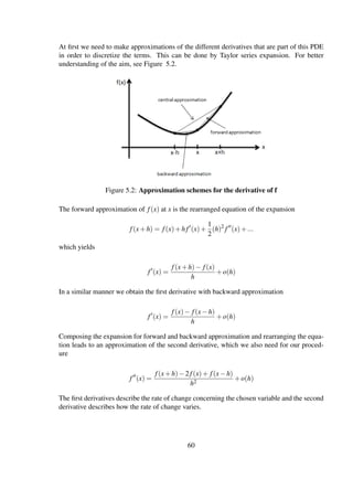
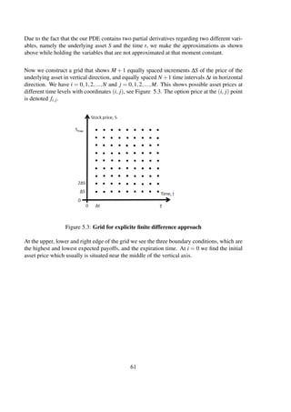
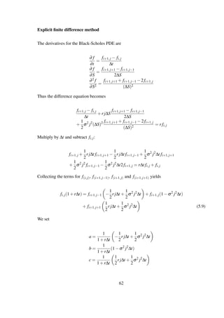
![and obtain the final equation
fi,j = aj fi+1,j−1 +bj fi+1,j +cj fi+1,j+1
We have established a method that shows the relation between the option value at time t and
the three possible values for time t +1. The values for a, b and c less the discount factor 1
1+r∆t
can be interpreted as the probabilities of an increased, decreased or unchanged price of the
underlying asset within one time interval ∆t. If we sum the probabilities we should obtain the
value of 1 which is easily checked and turns out to be true. Moreover 1
1+r∆t is the well known
approximation of e−r∆t.
The equation for calculation in trinomial tree can thus be expressed as
1+r∆t f(t) = er∆t
f(t) = [pu fu(t +1)+ pm fm(t +1)+ pd fd(t +1)] 0 ≤ t ≤ T −1 (5.10)
f(t) = e−r∆t
[pu fu(t +1)+ pm fm(t +1)+ pd fd(t +1)] 0 ≤ t ≤ T −1 (5.11)
From here the computations for trinomial trees are the same as for binomial trees adapted to
three probabilities.
Here we showed that backward approximation in the explicit finite difference method leads
to (5.11). In the Section 2.7, we showed how to obtain the equivalent formula for binomial
trees (2.24) using the backward formula derived through conditional expectation. These are
two principles yielding equivalent outcomes which is an interesting and comforting discov-
ery.
5.6 The case of binomial and trinomial equivalence
During the investigation of trinomial trees we came across a really interesting paper written
by Rubinstein [18]. This section demonstrates how he proceeded in order to find equivalence
between binomial and trinomial trees.
If we study Figure 5.1 again, we can make an interesting observation. Suppose that we double
the size of a time step and that we therefore arrive at nodes (2,4), (2,2) and (2,0) after one
∆t. We can see that this a trinomial single period tree. This must mean that we can compute
the value of an American option at t(0) either by one (5.11) or three equations [where (1,2) is
determined through (2,4) and (2,2); (1,0) through (2,2) and (2,0) and finally (0,0) through
(1,2) and (1,0)], using (2.24) iteratively.
63](https://image.slidesharecdn.com/056831bc-2170-4601-b463-4525efb79d14-150711133700-lva1-app6892/85/Bachelor-Thesis-Report-65-320.jpg)
![With that in mind, we can introduce the following equations where the left hand sides represent
the two time period nodes for the binomial tree, and the right hand sides represent the single
time period nodes for the overlapping trinomial tree.
fuu = fU fud = fM fdd = fD (5.12)
Now we use the equation that was derived in the explicit finite difference method, accepting
that the compound factor in (5.10) which is (1 + r∆t) can be substituted by 1 + ln(r)∆t (as
proposed by Rubinstein 2000 [18]). To make the derivation easier to read, we will denote
∆t = h and 2∆t = 2h.
[1+(lnr)2h]f0 = PU fU +(1−PU −PD)fM +PD fD
Recalling that we jump over one step for the binomial part of the tree we have
r2
f0 = p2
fuu +2p(1− p)fud +(1− p)2
fdd
Due to the presumed equivalence between the two ways of expressing the same states, we also
have
r2
= (1+lnr)2h
Since the trinomial interval has twice the size of one binomial it follows that
R = r2
= [1+2(lnR)h]1/2
(5.13)
Furthermore it should also be valid to claim that
p2
= PU, (1− p) = PD, 2p(1− p) = (1−PU −PD)
Due to the fact that one period in trinomial spacing (U,1,D) is double the size of one period
in binomial spacing, it is applicable to set
U = u2
, D = d2
, 1 = ud ⇒ d =
1
u
From (5.13) we get
r = [1+2(lnr)]
From the CRR model [4] we have
64](https://image.slidesharecdn.com/056831bc-2170-4601-b463-4525efb79d14-150711133700-lva1-app6892/85/Bachelor-Thesis-Report-66-320.jpg)
![p =
1
2
+
1
2
µ
√
h
σ
From Kamrad and Ritchken [11] we have
PU =
1
2λ2
+
1
2λ
µ
√
2h
σ
(5.14)
and
PD =
1
2λ2
−
1
2λ
µ
√
2h
σ
(5.15)
According to Rubinstein [18] we perform a little algebra and obtain
p =
1
2
1
2(σ2h− µ2h2)
+
1
σ2h− µ2h2
µ
√
2h
σ
1
2
(5.16)
We define for (5.14)
a ≡
1
2λ2
, b ≡
1
2λ
µ
√
2h
σ
⇒ b2
=
1
2λ2
µ2h
σ2
and can write that
PU = a+b ⇒ p2
= a+b (5.17)
If the two models are equivalent we should obtain from (5.15)
PD = (1− p)2
= a−b
This will not be true, unless if we choose that
u = e
√
σ2h−µ2h
(5.18)
According to Kamrad and Ritchken [11] we have
U = eλσ
√
2h
65](https://image.slidesharecdn.com/056831bc-2170-4601-b463-4525efb79d14-150711133700-lva1-app6892/85/Bachelor-Thesis-Report-67-320.jpg)
![From this follows that
u2
= eλσ
√
2h
(2lnu)2
= λ2
σ2
(2h)
λ2
=
σ22h
(2lnu)2
1
2λ2
=
1/4(σ2h)
(lnu)2
Now we substitute what we proposed in (5.18) into the last equation which yields
1
2λ2
=
(1/4)σ2
σ2 − µ2h
(5.19)
Now we set
a−b2
=
1
2λ2
−
1
2λ2
µ2h
σ
2
=
1
2λ2
σ2 − µ2h
σ2
and substitute
1
2λ2
with the right hand side of (5.19). That gives
(1/4)σ2
σ2 − µ2h
1
2λ2
σ2 − µ2h
σ2
=
1
4
Therefore
a−b2
=
1
4
⇒ a = b2
+
1
4
From (5.17) we have
p =
√
a+b
We plug in our expression for a and obtain
p = b2 +b+
1
4
= b+
1
2
From this follows
(1− p)2
=[1−(b+
1
2
)]2
= 1−2(b+
1
2
)+(b+
1
2
)2
=1−2b−1+b2
+b+
1
4
= b2
+
1
4
−b = a−b
66](https://image.slidesharecdn.com/056831bc-2170-4601-b463-4525efb79d14-150711133700-lva1-app6892/85/Bachelor-Thesis-Report-68-320.jpg)
![This means that (1− p)2 = a−b under condition u = e
√
σ2h−µ2h2
.
Therefore we can draw the conclusion that binomial models, with every other period skipped,
and trinomial models, under lognormal transformation, coincide if we choose
u = e
√
σ2h−µ2h
and
p =
1
2
1
2(σ2h− µ2h2)
+
1
σ2h− µ2h2
µ
√
2h
σ
1
2
as the parameters. This leads to a more efficient algorithm because fewer calculations are
necessary in order to price an American option as explained in the beginning of this sec-
tion.
5.7 More on the connection between binomial and trinomial
trees
This way of overlapping in the previous section implies also that we can use the Cox, Ross,
Rubinstein parameters u = eσ
√
∆t, d = e−σ
√
∆t and p∗ see (2.7) if volatility is constant, i.e., the
spacing between the nodes is of the same distance. In Derman et al [5] we found support for
that.
Taking into consideration that we jump over one time interval in the binomial part of the tree
and summing the above parameters, we obtain values for
p1 =
er∆t/2 −e−σ
√
∆t/2
eσ
√
∆t/2
−e−σ
√
∆t/2
2
p3 =
eσ
√
∆t/2
−er∆t/2
eσ
√
∆t/2
−e−σ
√
∆t/2
2
p2 = 1− p1 − p3
This result can give a base for the state space of implied trinomial trees but it is not the only
one. Another method was for instance developed by Jarrow and Rudd [10].
’Implied’ tree means that the volatility differs from time step to time step thus giving unequal
spacing between nodes. These kind of trees can match prices of standard options better than
constant volatility trees because the state space is chosen in advance which helps out with
fact that we discovered in Boyle’s approach where we had two constraints and five unknowns.
67](https://image.slidesharecdn.com/056831bc-2170-4601-b463-4525efb79d14-150711133700-lva1-app6892/85/Bachelor-Thesis-Report-69-320.jpg)

![Black-Scholes model than for example the Cox, Ross and Rubinstein model.
In Chapter 5, we extended the binomial model by adding the possibility of movements into
a third direction. Thus we established the trinomial model, its probability distribution and
properties. We continued with the presentation of Boyle’s method [2] to derive transition
probabilities. As for the binomial model we showed furthermore that we can obtain differ-
ent results depending on the choice of approximation technique for the discretization of the
continuous distribution, and how the random variable, that describes the return of the under-
lying security, is chosen to be distributed with its corresponding mean and variance. We also
made an attempt to derive the risk neutral probability and discovered that there is no unique
probability distribution that generates a contingent claim in the replicating portfolio. We also
demonstrated how the Black-Scholes partial differential equation can be discretized and fur-
ther processed so that an option value equation is obtained. This trinomial equation is the
equivalent to the binomial option pricing formula which we obtained through conditional ex-
pectation in the Chapter 2. This similarity through different methods stroke us as interesting
and we looked deeper into this seemingly present connection. The result that we showed in
part 5.6 states that the binomial option pricing model and the explicit finite difference method
coincide under a certain parametrization. We then extended our thoughts about the connection
of binomial and trinomial models because we discovered that there are models assuming con-
stant volatility and models assuming varying volatility. Therefore we give a brief introduction
to implied trinomial trees which closes the work on this paper.
However, we are not satisfied. Many of our topics have the potential to be investigated further
and more models should be examined. For example we would like to know if there are more
theories about the speed of convergence of the binomial model to the Black-Scholes formula.
We were happy to find the Leisen - Reimer model that converges faster as the CRR model,
but are there models that are even faster and does the trinomial model converge as well? It
would also have been interesting to do some numerical computations and to see if binomial
models, trinomial models and the Black-Scholes formula will produce the same results. Also,
how big is the approximation error and how many time steps need to be implemented into the
respective models in order to obtain similar results?
Besides we have only studied the basic ideas of option pricing. As it was mentioned before,
there exists lots of different kinds of options in the market. We can use our current know-
ledge and the basic algorithm of option pricing to learn more about different kinds of options
in future studies. Firstly, in our approach we have not covered jump diffusion, which is an
important dilemma in option pricing. Merton [15] has already done that, so working in option
pricing with jump diffusion and expanding it in different models would be really vital and
interesting. Then, we can study Asian options, non-standard American options, Swap options,
Barrier options and Currency options [7]. Additionally, if we look at markets where there exist
some complicated options, we have to estimate their price by a numerical approach, namely
Monte Carlo and Quasi-Monte Carlo Simulation [6]. So, one further step in future studies
could be this matter. It is an important subject because if we want to do estimations we will
have some errors and consequently we will have to use our knowledge from Statistical In-
ferences [21],[6] to find confidence intervals, conduct some different statistic tests to find the
70](https://image.slidesharecdn.com/056831bc-2170-4601-b463-4525efb79d14-150711133700-lva1-app6892/85/Bachelor-Thesis-Report-72-320.jpg)
![for development of software that is able to estimate option prices and this is a field that is still
developing.
6.1.2 Objective 2 - Ability to search, collect, evaluate and interpret
The topic for this thesis is very theoretical and it was crucial to scan many papers in order to
find the results that we were looking for. It was even more important to realize what we were
reading for understanding why we found so many different results. We had to use text books
as for example [7] and [21], and also lecture notes [14], [17], with the purpose of really getting
a grip on the derivations. An example that really emphasizes this is the demonstration of the
case of binomial and trinomial equivalence in Section 5.6. The paper by Rubinstein referred to
the Explicite Finite Difference approach by Brennan and Schwartz. We found it important to
have an understanding of this paper in order to properly understand Rubinstein, so we studied
Brennan and Schwartz as well (which is represented in Section 5.5). This paper in turn was
hard to understand so we had to search in one of our textbooks [7] as well. This helped very
much but was not sufficient why we consulted a book from our course in Calculus as well.
Similar approaches applied to contents in other sections and in that way we collected sources
and aggregated the contents of the thesis.
6.1.3 Objective 3 - Identify, formulate and solve problems
In the first year of our program, we came (among others) across option pricing formulas,
binomial models and the Black-Scholes formulae in Introduction to financial mathematics.
We wondered how up and down factors were set, probabilities were determined and on what
ground the size of time intervals were chosen, but we did not have sufficient knowledge to
understand this. Therefore, the problem formulation of this thesis is a follow up on questions
that we already wanted to get answers to in the past. As we found out and explained care-
fully, there are different ways for solving these problems as we have shown throughout this
thesis.
6.1.4 Objective 4 - Communication of our project to different groups
We believe that our thesis can be read and understood by a range of people with varying
previous knowledge about option pricing and the mathematics behind it. The reader that is
interested in an overview of options and how they are priced can be satisfied with Sections
2.1, 2.3 - 2.4 and 2.7 - 2.9, whereas the more interested financial economist can include the
rest of Chapter 2 and Chapters 4 and 5, or at least the results provided at their end. The
mathematician might be more interested in calculations, but should be able to understand the
financial background as well. A financial analyst or engineer will grasp the whole thesis.
72](https://image.slidesharecdn.com/056831bc-2170-4601-b463-4525efb79d14-150711133700-lva1-app6892/85/Bachelor-Thesis-Report-74-320.jpg)

![Bibliography
[1] Fischer Black and Myron Scholes. The pricing of options and corporate liabilities.
Journal of Political Economy, 81(3):pp. 637–654, 1973.
[2] Phelim P. Boyle. A lattice framework for option pricing with two state variables. The
Journal of Financial and Quantitative Analysis, 23(1):pp. 1–12, 1988.
[3] Michael J. Brennan and Eduardo S. Schwartz. Finite difference methods and jump pro-
cesses arising in the pricing of contingent claims: A synthesis. The Journal of Financial
and Quantitative Analysis, 13(3):pp. 461–474, 1978.
[4] John C Cox, Stephen A Ross, and Mark Rubinstein. Option pricing: A simplified ap-
proach. Journal of financial Economics, 7(3):229–263, 1979.
[5] Emanuel Derman, Iraj Kani, and Neil Chriss. Implied trinomial tress of the volatility
smile. The Journal of Derivatives, 3(4):7–22, 1996.
[6] Paul Glasserman. Monte Carlo methods in financial engineering. Springer, New York,
2004.
[7] John Hull. Options, futures, and other derivatives. Pearson Prentice Hall, Upper Saddle
River, NJ, 2009.
[8] George M. Jabbour, Marat V. Kramin, and Stephen D. Young. Two-state option pricing:
Binomial models revisited. Journal of Futures Markets, 21(11):987–1001, 2001.
[9] Robert Jarrow. Derivative securities. South-Western College Pub, Cincinnati, Ohio,
2000.
[10] Robert A Jarrow and Andrew Rudd. Option pricing. Dow Jones-Irwin Homewood, IL,
1983.
[11] Bardia Kamrad and Peter Ritchken. Multinomial approximating models for options with
k state variables. Management science, 37(12):1640–1652, 1991.
[12] Masaaki Kijima. Stochastic processes with applications to finance. Chapman and Hall
CRC, Boca Raton, Fla, 2003.
74](https://image.slidesharecdn.com/056831bc-2170-4601-b463-4525efb79d14-150711133700-lva1-app6892/85/Bachelor-Thesis-Report-76-320.jpg)
![[13] Dietmar PJ Leisen and Matthias Reimer. Binomial models for option valuation-
examining and improving convergence. Applied Mathematical Finance, 3(4):319–346,
1996.
[14] Anatoliy Malyarenko. Lecture notes, Stochastic Processes. 2012.
[15] Robert C. Merton. Theory of rational option pricing. The Bell Journal of Economics and
Management Science, 4(1):pp. 141–183, 1973.
[16] Jr. Rendleman, Richard J. and Brit J. Bartter. Two-state option pricing. The Journal of
Finance, 34(5):pp. 1093–1110, 1979.
[17] Jan Röman. Lecture notes, Analytical Finance I. http://janroman.dhis.org/, 2012.
[18] Mark Rubinstein. On the relation between binomial and trinomial option pricing models.
The Journal of Derivatives, 8(2):47–50, 2000.
[19] Yisong Tian. A modified lattice approach to option pricing. Journal of Futures Markets,
13(5):563–577, 1993.
[20] Lenos Trigeorgis. A log-transformed binomial numerical analysis method for valuing
complex multi-option investments. The Journal of Financial and Quantitative Analysis,
26(3):pp. 309–326, 1991.
[21] Dennis Wackerly. Mathematical statistics with applications, 7th edition. Thomson
Brooks/Cole, Belmont, CA, 2008.
75](https://image.slidesharecdn.com/056831bc-2170-4601-b463-4525efb79d14-150711133700-lva1-app6892/85/Bachelor-Thesis-Report-77-320.jpg)
![Appendix A
Appendix
In this paper we have used Black-Scholes model 1973 and their result several times. So, it
might be a good idea to see how they obtain their formula. To begin with, we explain the
derivation of Black-Scholes partial differential equation (PDE)and then we will derive Black-
Scholes formula for European Call Option [1],[17]. We got a considerable help from lecture
notes of the course "Analytical Finance I" [17] which we have studied in our program to
explain these derivations properly.
A.1 Black-Scholes PDE
Again, we consider a market which consist of two type of financial instruments, bond and
stocks. So, we will have [1],[17]:
dB(t) = rB(t)dt
B(0) = 1
Which means the return on bound is simply B(t) = ert. And we assume that the stock price
will follow the following stochastic process [1],[17]:
dS(t) = αS(t)dt +σS(t)dW
S(0) = S0
Where, in deterministic part α is drift coefficient and in stochastic part which follows Geomet-
ric Brownian Motion (Wiener Process), σ is diffusion coefficient. Now, we can construct our
portfolio h = (hB,hS), where hB represents the number of bond and hS represents the number
of stocks. So, the value process will be defined as [1],[17]:
V(t) = hB(t)B(t)+hS(t)S(t)
76](https://image.slidesharecdn.com/056831bc-2170-4601-b463-4525efb79d14-150711133700-lva1-app6892/85/Bachelor-Thesis-Report-78-320.jpg)
![and to have our portfolio self-financed we must have [1],[17]:
dV(t) = hB(t)dB(t)+hS(t)dS(t)
Moreover, we have invested our money in two categories stock and bond. Let’s say we have
decided to invest x percent of our money in bond and y percent of our money in stock. x and y
can get negative value, since its possible to short one of securities to long the other, but under
condition x +y = 1. To hold this condition, we define a relative portfolio u = (x,y) in such a
way that x(t)+y(t) = 1 holds. So, we will obtain following relative portfolio [1],[17]:
x(t) = hB(t)B(t)
V ⇒ hB = xV
B
y(t) = hS(t)S(t)
V ⇒ hS = yV
S
rewriting the self-financed process equation in terms of the relative portfolio and substituting
the value of dB and dS we will obtain [1],[17]:
dV = V(rx+αy)dt +V(σy)dW (A.1)
Moreover, if we suppose V(t) = V(t,S(t)) we can apply Itô formula and we will obtain
[1],[17]:
dV =
∂V
∂t
dt +
∂V
∂S
dS+
1
2
∂2V
∂S2
(dS)2
= Vtdt +VS(αSdt +σSdW)+
1
2
VSSσ2
S2
(dW)2
substituting (dt)2 = 0, (dW)2 = dt, collecting the terms which are multiplying by dt and
multiplying right hand side by V/V we will obtain [1],[17]:
dV =
V Vt +VSαS+ 1
2VSSσ2S2 dt
V
+
V(VsσS)dW
V
(A.2)
comparing (A.1) and (A.2), we will obtain:
y =
VSS
V
rx+αy =
Vt +VSαS+ 1
2VSSσ2S2
V
substituting y =
VSS
V
in (A.2), we will obtain:
dV = V
Vt + 1
2VSSσ2S2
V
+αy dt +VyσdW
77](https://image.slidesharecdn.com/056831bc-2170-4601-b463-4525efb79d14-150711133700-lva1-app6892/85/Bachelor-Thesis-Report-79-320.jpg)
![if we just multiply
Vt + 1
2VSSσ2S2
V
by r/r, we will get:
dV = V r
Vt + 1
2VSSσ2S2
rV
+αy dt +VyσdW
comparing the last equation with (A.1) will give us:
x =
Vt + 1
2VSSσ2S2
rV
and since x+y = 1:
Vt + 1
2VSSσ2S2
rV
+
SVS
V
= 1
multiplying both hand side with rV will give us Black-Scholes PDE:
Vt +rSVS +
1
2
VSSσ2
S2
= rV
It is common to write Black-Scholes PDE as [1],[17]:
Θ+rS∆+
1
2
Γσ2
S2
= rV (A.3)
Where [1],[17]:
Θ =
∂V
∂t
, represents the change in value with respect to the time
rS∆ = rS
∂V
∂S
, represents the change in value with respect to stock price
1
2
Γσ2
S2
=
1
2
σ2
S2 ∂V
∂S
, represents the change in value with respect to volatility of stock price
rV, represents the expected return, which means in risk-neutral world the expected return must
be equal to risk-free interest rate.
A.2 Black-Scholes formula for European Call option
In this section we will try to go through Black and Scholes approach to find the fair price of
European call option. We have already derived the Black-Scholes PDE and we know that the
payoff to the European call option is max(ST −K,0). So we can write [1],[17]:
Vt +rSVS + 1
2VSSσ2S2 = rV
VT = max(ST −K,0)
78](https://image.slidesharecdn.com/056831bc-2170-4601-b463-4525efb79d14-150711133700-lva1-app6892/85/Bachelor-Thesis-Report-80-320.jpg)
![To solve this PDE, we can use a trick. Using this trick we suppose the V(t,S(t)) is solution to
Black-Scholes PDE. where the stock price following the stochastic process [1],[17]:
dS(t) = αS(t)dt +σS(t)dW
S(0) = S0
Applying Itô formula to V(t,S(t)), we will obtain [1],[17]:
dV =
∂V
∂t
dt +
∂V
∂S
dS+
1
2
∂2V
∂S2
(dS)2
= Vtdt +VS(αSdt +σSdW)+
1
2
VSSσ2
S2
(dW)2
= Vt +rSVs +
1
2
VSSσ2
S2
dt +σSVSdW
where Itô formula gives α = r, (dt)2 = 0 and (dW)2 = dt. SubstitutingVt +rSVs + 1
2VSSσ2S2 =
rV, we will obtain:
dV = rVdt +σSVSdW
taking integral:
T
t
dV =
T
t
(rV(u)du+σS(u)VS(u)dW(u))
VT −Vt = r
T
t
V(u)du+σ
T
t
S(u)VS(u)dW(u)
taking expectation will yield:
E[VT −Vt] = E r
T
t
V(u)du+σ
T
t
S(u)VS(u)dW(u)
since the expectation of a sum is the sum of expectation, the expectation of a constant is
just that constant, i.e., E[Vt] = Vt and the expectation of stochastic part is zero, we will ob-
tain:
E[VT ] = Vt +r
T
t
E[V(u)]du+0
denoting E[VT ] = m and taking derivative of both hand side with respect to time, we can use
the fundamental theorem of calculus and we will obtain:
m = Vt +r
T
t
mdu
⇒
dm
dt
= 0+rm
⇒
dm
m
= rdt
79](https://image.slidesharecdn.com/056831bc-2170-4601-b463-4525efb79d14-150711133700-lva1-app6892/85/Bachelor-Thesis-Report-81-320.jpg)
![solving this differential equation we will obtain:
T
t
dm
m
= r
T
t
dt
⇒ln(mT −mt) = r(T −t)
⇒mT = mter(T−t)
⇒E[VT ] = Vter(T−t)
⇒Vt = e−r(T−t)
E[VT ]
since VT = max{ST −K,0} and random variable ST follows the stochastic process under equi-
valent martingale probability measure, we can write [1],[17]:
c(t,S(t)) = V(t,S(t)) = e−r(T−t)
EQ
[max{ST −K,0}|Ft]
which implies that the fair price, c(t,S(t)) of an European Call Option under martingale
probability measure , is discounted expected payoff. Now, we have the formula to calcu-
late the price of European call option. The next step is to find the equation for ST . Let denote
X(t) = lnS(t), where we know our process has the following form.
dS(t) = rS(t)dt +σS(t)dW
S(0) = S0
applying Itô formula, we will obtain [1],[17]:
dX =
∂X
∂t
dt +
∂X
∂S
dS+
1
2
∂2X
∂S2
(dS)2
= 0+
1
S
(rSdt +σSdW)+
1
2
−1
S2
σ2
S2
(dW)2
= r −
1
2
σ2
dt +σdW
taking the integral we will obtain:
XT −Xt = r −
1
2
σ2
(T −t)+σ(WT −Wt)
substituting X(t) = lnS(t) and taking exponent of both hand side we will obtain:
ST = Ste(r−1
2 σ2
)(T−t)+σ(WT −Wt)
since we want the price process to follow a Geometric Brownian Motion, the Wiener pro-
cess part can be re-written as WT −Wt =
√
T −tz where, z ∼ N r − 1
2σ2 (T −t),σ2(T −t)
[1],[17].
80](https://image.slidesharecdn.com/056831bc-2170-4601-b463-4525efb79d14-150711133700-lva1-app6892/85/Bachelor-Thesis-Report-82-320.jpg)
![Remark A.2.1. The current explanation can make it clear why Black and Scholes, and Merton
considered that dynamic of risky asset or stock is following the Geometric Brownian Motion.
As we saw, with this assumption we can find a random variable U such that our random
variable will have normal distribution, i.e., U ∼ N r − 1
2σ2 (T −t),σ2(T −t) . Having a
normal random variable U we can transform our random variable to standard normal random
variable Z by letting Z = U−µ
σ [21] where µ stands for mean and σ is standard deviation and
then, we can use normal cure areas to find the probability.
In next step, we will introduce the following notations:
˜r = r −
1
2
σ2
τ = T −t
√
τz = WT −Wt
y = ˜rτ +σ
√
τz ⇒ z =
y− ˜rτ
σ
√
τ
ST = Stey
Now, if we calculate ST −K we will obtain, y0 = ln
K
St
. So, we introduce new point
z0 =
ln K
St
− ˜rτ
σ
√
τ
. Substituting, all notation above we can calculate the price of European Call
Option.
c(t,S(t)) = V(t,S(t)) = e−r(T−t)
EQ
[max{ST −K,0}|Ft]
= e−rτ
∞
−∞
max(ST −k,0)φ(z)dz
= e−rτ
∞
z0
(ST −k)φ(z)dz
= e−rτ
∞
z0
(Stey
−k)φ(z)dz
we know that for standard normal distribution function, the cumulative distribution function
81](https://image.slidesharecdn.com/056831bc-2170-4601-b463-4525efb79d14-150711133700-lva1-app6892/85/Bachelor-Thesis-Report-83-320.jpg)
![is φ(z) = 1√
2π
e−z2/2. substituting we will get:
c(t,S(t)) =
e−rτ
√
2π
∞
z0
(Stey
−k)e−z2/2
dz
=
Ste−rτ
√
2π
∞
z0
ey−z2/2
dz−
ke−rτ
√
2π
∞
z0
e−z2/2
dz
=
Ste−rτ
√
2π
∞
z0
ey−z2/2
dz−ke−rτ
N(−z0)
=
Ste−rτ
√
2π
∞
z0
e˜rτ+σ
√
τz−z2/2
dz−ke−rτ
N(−z0)
=
Ste−rτe−˜rτ
√
2π
∞
z0
e−(z−σ
√
τ)2/2
eσ2τ
dz−ke−rτ
N(−z0)
=
Ste0
√
2π
∞
z0
e−(z−σ
√
τ)2/2
dz−ke−rτ
N(−z0)
= StN −z0 +σ
√
τ −ke−r(T−t)
N (−z0)
To summarize we can calculate the price of a European Call option using the following for-
mula [1],[17]:
c(t,S(t)) = StN (d1)−Ke−r(T−t)
N (d2)
d1 =
ln St
K + r + 1
2σ2 (T −t)
σ (T −t)
d2 =
ln St
K + r − 1
2σ2 (T −t)
σ (T −t)
= d1 −σ (T −t)
With the similar approach we can find the price of European Put Option, i.e., p(t,S(t)), where
the payoff is max(K −ST ,0) [1],[7],[17].
p(t,S(t)) = Ke−r(T−t)
N (−d2)StN (−d1)
Remark A.2.2. As we explained in previous remark, Black-Scholes formula has a big advant-
age. So, for pricing European call and put options we need to calculate the value for d1 and
d2 and then we can find the value for N(d1) and N(d1) from standard normal random vari-
able table. Finally, substituting inputs we can calculate the fair price of European Call or put
options.
Remark A.2.3. For pricing American put option, because of the possibility of early exercises,
we do not have a widely used formula. One needs to use some numerical method like Monte-
Carlo simulation [6] to simulate the process and estimate the price or in simple cases, it is
possible to use the backward equation to calculate the price of American put option via lattice
approach.
82](https://image.slidesharecdn.com/056831bc-2170-4601-b463-4525efb79d14-150711133700-lva1-app6892/85/Bachelor-Thesis-Report-84-320.jpg)


![Senior Project [Hien Truong, 4204745]](https://cdn.slidesharecdn.com/ss_thumbnails/a82856d9-6fc7-4bef-9d6b-c3ea4bbadfc0-150720053419-lva1-app6892-thumbnail.jpg?width=640&height=640&fit=bounds)