International Journal of Mechanical Engineering Research and Development (IJMERD), ISSN 2248
– 9347(Print) ISSN 2228 – 9355(Online), Volume 1, Number 1, January - April (2011)
60
STUDY THE DIFFERENT FEEDBACK METHODS IN
MANUFACTURING SETUP ERRORS FOR CONSTANT AND
RANDOM VARIABLES
S Y Gajjal Dr. M D Jaybhaye Dr. A P S Gaur
Asst. Prof.SCOE, Pune Asso. Prof.,COE, Pune Prof. BU, Jhansi
ABSTRACT
The performance criteria is the quadratic off-target cost incurred over a small
number of parts produced. Analytical formulae are presented and numerically illustrated.
Two cases are considered, the first one where the setup error is constant but unknown
offset and the second one where the setup error is a random variable with unknown first
two moments. It is shown how Grubbs’ harmonic rule and a simple integral provide a
robust adjustment strategy in a variety of circumstances. As a by-product, the formulae
presented in this paper allow to compute the expected off-target quadratic cost when a
sudden shift occurs during production (not necessarily at setup) and the adjustment
scheme compensates immediately after its occurrence.
1. INTRODUCTION
Suppose that due to a defective setup machine operation, the quality
characteristic generated by a production process is in state of statistical control but the
process starts off-target. Adjusting the process is justified if the only relevant cost is the
cost of running the process off-target. Sequential adjustment rules for this problem were
proposed by Grubbs (1983). These rules have been shown to derive from much broader
class of setup adjustment problems based on stochastic control methods by Del Castillo,
Pan and Colosimo (2002). In this paper, the small sample performance of Grubbs
adjustment rules are studied and contrasted with other feedback adjustment methods.
To introduce some basic notation that will be based in that follows, let Yt denote
the observed derivation from target of some quality characteristic of interest, following
Grubbs (1983), a simple but useful model for the setup adjustment problem is to assume
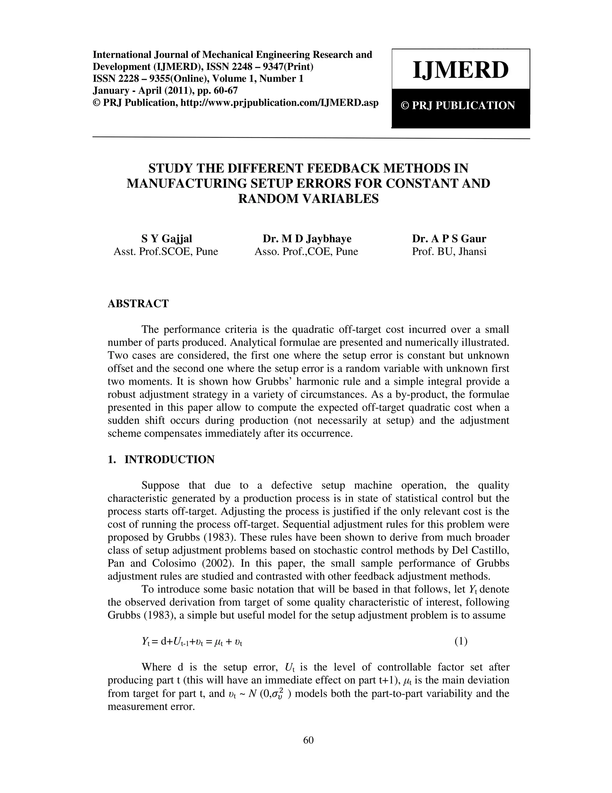
Yt = d+Ut-1+υt = µt + υt (1)
Where d is the setup error, Ut is the level of controllable factor set after
producing part t (this will have an immediate effect on part t+1), µt is the main deviation
from target for part t, and υt ~ N (0,ߪజ
ଶ
) models both the part-to-part variability and the
measurement error.
IJMERD
© PRJ PUBLICATION
International Journal of Mechanical Engineering Research and
Development (IJMERD), ISSN 2248 – 9347(Print)
ISSN 2228 – 9355(Online), Volume 1, Number 1
January - April (2011), pp. 60-67
© PRJ Publication, http://www.prjpublication.com/IJMERD.asp
International Journal of Mechanical Engineering Research and Development (IJMERD), ISSN 2248
– 9347(Print) ISSN 2228 – 9355(Online), Volume 1, Number 1, January - April (2011)
61
Two different control rules were derived by Grubbs depending on two sets of
assumptions made on setup error d:
1. If d is an unknown constant, minimization of Var(µn+1 ) subject to E [µn+1]=0 results
in Grubbs’ “harmonic rule” :Ut = -݀መt,
݀መt=݀መt-1+KtYt (2)
Kt = 1/t
Or
Ut - Ut-1 = ▽Ut =-
௒୲
୲
Thus the weights Kt follow a harmonic series. An initial (a priori) estimate ݀መ0 is
required to set the first setting of the controllable factor at U0 = -݀መ0. Del Castillo, Pan
and Colosimo (2002) point out how adjustment rules (2) is a particular case of
Robbins and Monro’s (1951) celebrated stochastic approximation method.
Therefore, this paper contains (indirectly) a small-sample performance study of
stochastic approximation methods applied to the simple case of estimation of an
unknown constant.
2. If d ~ N (݀ҧ,ߪజ
ଶ
) the both ݀ҧ and ߪௗ
ଶ
known, minimization of E [Σ௧ୀଵ
௡
ߤ௧
ଶ
] is achieved
by Grubbs second adjustment rule. In this case,
3.
݀መt = ݀መt-1 + KtYt , Kt =
ଵ
௧ା
഑ഔ
మ
഑೏
మ
and ▽Ut= - KtYt (3)
This rule is called Grubbs’ “extended” rule by Trietsch (1998).
Kt =
ଵ
௧ା
഑ഔ
మ
഑೏
మ
, and ▽Ut= - KtYt (4)
The interpretation is that, a priori, d ~ (݀መ0, P0). Thus for Grubbs’ extended
rule to be optimal with respect to E [Σ௧ୀଵ
௡
ߤ௧
ଶ
] we need to know ݀ҧ (so we can set ݀ҧ0 =
݀ҧ) and ߪௗ
ଶ
and ߪజ
ଶ
must be known for us to use (3). Evidently, if P0 = ߪௗ
ଶ
, (3) and (4)
are identical. Note how under this interpretation, if there is no prior information on
offset (P0 → ∞) is equivalent to (2), Grubbs’ simpler harmonic rule.
An additional adjustment rule that will be contrasted is an integral controller
(Box and Luceno 1997);
▽Ut= - λYt (5)
Which, contrary to Grubbs’ rules, does not converge to zero since λ is a constant.
International Journal of Mechanical Engineering Research and Development (IJMERD), ISSN 2248
– 9347(Print) ISSN 2228 – 9355(Online), Volume 1, Number 1, January - April (2011)
62
2. PERFORMANCE INDICES FOR SS
The Performance indices that will be used in the reminder of this paper are
presented in this section for the two cases considered by Grubbs.
Consider first the case where the setup error d is an unknown constant or
“offset”. For this case, performance index considered is the scaled Average Integrated
Square Deviation (AISD) incurred over m time instants or parts. This is defined for
integer m > 0 as:
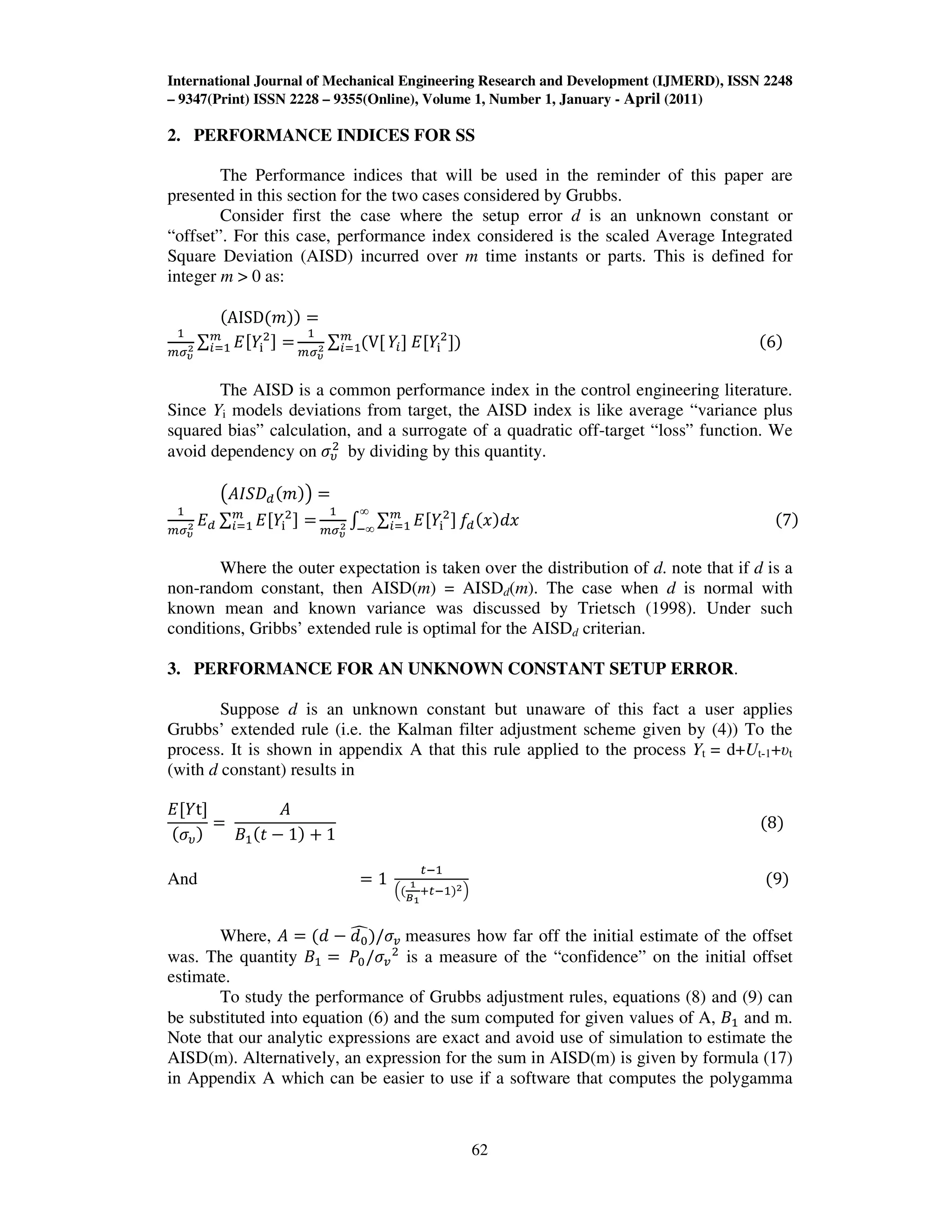
ሺAISDሺ݉ሻሻ ൌ
ଵ
௠ఙഔ
మ ∑ ‫ܧ‬ሾܻ୧
ଶሿ ൌ௠
௜ୀଵ
ଵ
௠ఙഔ
మ ∑ ሺVሾ௠
௜ୀଵ ܻ௜ሿ ‫ܧ‬ሾܻ୧
ଶ
ሿሻ ሺ6ሻ
The AISD is a common performance index in the control engineering literature.
Since Yi models deviations from target, the AISD index is like average “variance plus
squared bias” calculation, and a surrogate of a quadratic off-target “loss” function. We
avoid dependency on ߪజ
ଶ
by dividing by this quantity.
൫‫ܦܵܫܣ‬ௗሺ݉ሻ൯ ൌ
ଵ
௠ఙഔ
మ ‫ܧ‬ௗ ∑ ‫ܧ‬ሾܻ୧
ଶ
ሿ ൌ௠
௜ୀଵ
ଵ
௠ఙഔ
మ ‫׬‬ ∑ ‫ܧ‬ሾܻ୧
ଶ
ሿ௠
௜ୀଵ
∞
ି∞
݂ௗሺ‫ݔ‬ሻ݀‫ݔ‬ ሺ7ሻ
Where the outer expectation is taken over the distribution of d. note that if d is a
non-random constant, then AISD(m) = AISDd(m). The case when d is normal with
known mean and known variance was discussed by Trietsch (1998). Under such
conditions, Gribbs’ extended rule is optimal for the AISDd criterian.
3. PERFORMANCE FOR AN UNKNOWN CONSTANT SETUP ERROR.
Suppose d is an unknown constant but unaware of this fact a user applies
Grubbs’ extended rule (i.e. the Kalman filter adjustment scheme given by (4)) To the
process. It is shown in appendix A that this rule applied to the process Yt = d+Ut-1+υt
(with d constant) results in
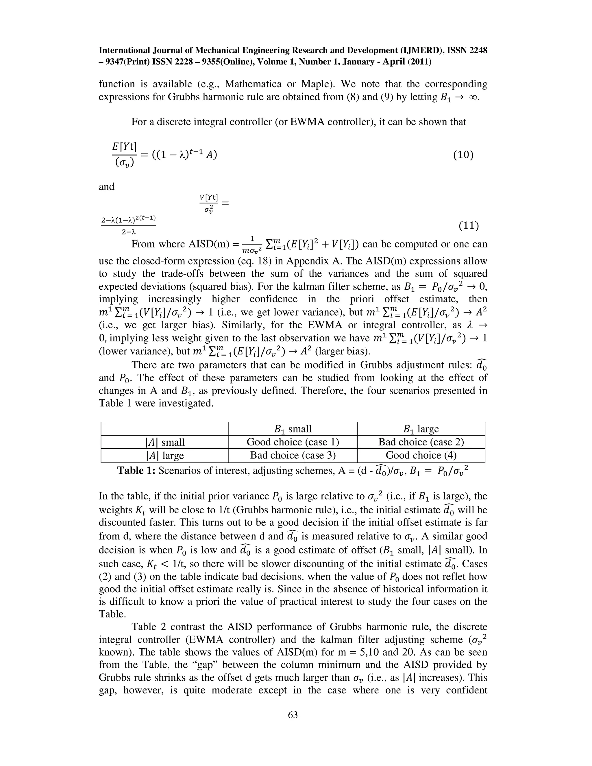
‫ܧ‬ሾܻtሿ
ሺߪజሻ
ൌ
‫ܣ‬
‫ܤ‬ଵሺ‫ݐ‬ െ 1ሻ ൅ 1
ሺ8ሻ
And ൌ 1
௧ିଵ
ቀሺ
భ
ಳభ
ା௧ିଵሻమቁ
ሺ9ሻ
Where, ‫ܣ‬ ൌ ሺ݀ െ ݀଴
෢ሻ/ߪ௩ measures how far off the initial estimate of the offset
was. The quantity ‫ܤ‬ଵ ൌ ܲ଴/ߪ௩
ଶ
is a measure of the “confidence” on the initial offset
estimate.
To study the performance of Grubbs adjustment rules, equations (8) and (9) can
be substituted into equation (6) and the sum computed for given values of A, ‫ܤ‬ଵ and m.
Note that our analytic expressions are exact and avoid use of simulation to estimate the
AISD(m). Alternatively, an expression for the sum in AISD(m) is given by formula (17)
in Appendix A which can be easier to use if a software that computes the polygamma
International Journal of Mechanical Engineering Research and Development (IJMERD), ISSN 2248
– 9347(Print) ISSN 2228 – 9355(Online), Volume 1, Number 1, January - April (2011)
63
function is available (e.g., Mathematica or Maple). We note that the corresponding
expressions for Grubbs harmonic rule are obtained from (8) and (9) by letting ‫ܤ‬ଵ ՜ ∞.
For a discrete integral controller (or EWMA controller), it can be shown that
‫ܧ‬ሾܻtሿ
ሺߪజሻ
ൌ ሺሺ1 െ λሻ௧ିଵ
‫ܣ‬ሻ ሺ10ሻ
and
௏ሾ௒୲ሿ
ఙഔ
మ ൌ
ଶିλሺଵିλሻమሺ೟షభሻ
ଶିλ
ሺ11ሻ
From where AISD(m) =
ଵ
௠ఙೡ
మ
∑ ሺ‫ܧ‬ሾܻ௜ሿଶ௠
௜ୀଵ ൅ ܸሾܻ௜ሿሻ can be computed or one can
use the closed-form expression (eq. 18) in Appendix A. The AISD(m) expressions allow
to study the trade-offs between the sum of the variances and the sum of squared
expected deviations (squared bias). For the kalman filter scheme, as ‫ܤ‬ଵ ൌ ܲ଴/ߪ௩
ଶ
՜ 0,
implying increasingly higher confidence in the priori offset estimate, then
݉ଵ ∑ ሺܸሾܻ௜ሿ/ߪ௩
ଶ
ሻ௠
௜ ୀ ଵ ՜ 1 (i.e., we get lower variance), but ݉ଵ ∑ ሺ‫ܧ‬ሾܻ௜ሿ/ߪ௩
ଶ
ሻ௠
௜ ୀ ଵ ՜ ‫ܣ‬ଶ
(i.e., we get larger bias). Similarly, for the EWMA or integral controller, as ߣ ՜
0, implying less weight given to the last observation we have ݉ଵ ∑ ሺܸሾܻ௜ሿ/ߪ௩
ଶ
ሻ௠
௜ ୀ ଵ ՜ 1
(lower variance), but ݉ଵ ∑ ሺ‫ܧ‬ሾܻ௜ሿ/ߪ௩
ଶ
ሻ௠
௜ ୀ ଵ ՜ ‫ܣ‬ଶ
(larger bias).
There are two parameters that can be modified in Grubbs adjustment rules: ݀଴
෢
and ܲ଴. The effect of these parameters can be studied from looking at the effect of
changes in A and ‫ܤ‬ଵ, as previously defined. Therefore, the four scenarios presented in
Table 1 were investigated.
‫ܤ‬ଵ small ‫ܤ‬ଵ large
|‫|ܣ‬ small Good choice (case 1) Bad choice (case 2)
|‫|ܣ‬ large Bad choice (case 3) Good choice (4)
Table 1: Scenarios of interest, adjusting schemes, A = (d - ݀଴
෢)/ߪ௩, ‫ܤ‬ଵ ൌ ܲ଴/ߪ௩
ଶ
In the table, if the initial prior variance ܲ଴ is large relative to ߪ௩
ଶ
(i.e., if ‫ܤ‬ଵ is large), the
weights ‫ܭ‬௧ will be close to 1/t (Grubbs harmonic rule), i.e., the initial estimate ݀଴
෢ will be
discounted faster. This turns out to be a good decision if the initial offset estimate is far
from d, where the distance between d and ݀଴
෢ is measured relative to ߪ௩. A similar good
decision is when ܲ଴ is low and ݀଴
෢ is a good estimate of offset (‫ܤ‬ଵ small, |‫|ܣ‬ small). In
such case, ‫ܭ‬௧ ൏ 1/t, so there will be slower discounting of the initial estimate ݀଴
෢. Cases
(2) and (3) on the table indicate bad decisions, when the value of ܲ଴ does not reflet how
good the initial offset estimate really is. Since in the absence of historical information it
is difficult to know a priori the value of practical interest to study the four cases on the
Table.
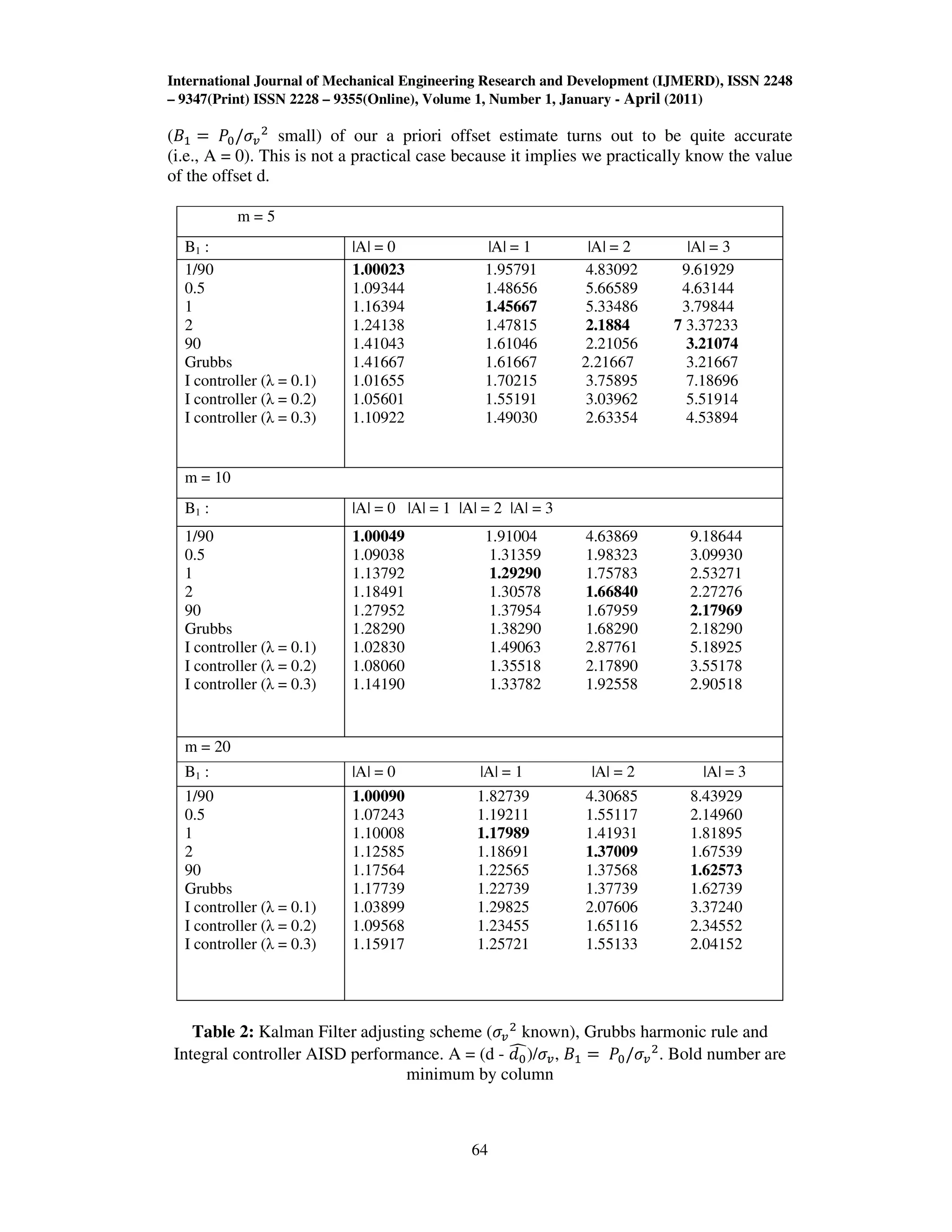
Table 2 contrast the AISD performance of Grubbs harmonic rule, the discrete
integral controller (EWMA controller) and the kalman filter adjusting scheme (ߪ௩
ଶ
known). The table shows the values of AISD(m) for m = 5,10 and 20. As can be seen
from the Table, the “gap” between the column minimum and the AISD provided by
Grubbs rule shrinks as the offset d gets much larger than ߪ௩ (i.e., as |‫|ܣ‬ increases). This
gap, however, is quite moderate except in the case where one is very confident
International Journal of Mechanical Engineering Research and Development (IJMERD), ISSN 2248
– 9347(Print) ISSN 2228 – 9355(Online), Volume 1, Number 1, January - April (2011)
64
(‫ܤ‬ଵ ൌ ܲ଴/ߪ௩
ଶ
small) of our a priori offset estimate turns out to be quite accurate
(i.e., A = 0). This is not a practical case because it implies we practically know the value
of the offset d.
m = 5
B1 : |A| = 0 |A| = 1 |A| = 2 |A| = 3
1/90
0.5
1
2
90
Grubbs
I controller (λ = 0.1)
I controller (λ = 0.2)
I controller (λ = 0.3)
1.00023 1.95791 4.83092 9.61929
1.09344 1.48656 5.66589 4.63144
1.16394 1.45667 5.33486 3.79844
1.24138 1.47815 2.1884 7 3.37233
1.41043 1.61046 2.21056 3.21074
1.41667 1.61667 2.21667 3.21667
1.01655 1.70215 3.75895 7.18696
1.05601 1.55191 3.03962 5.51914
1.10922 1.49030 2.63354 4.53894
m = 10
B1 : |A| = 0 |A| = 1 |A| = 2 |A| = 3
1/90
0.5
1
2
90
Grubbs
I controller (λ = 0.1)
I controller (λ = 0.2)
I controller (λ = 0.3)
1.00049 1.91004 4.63869 9.18644
1.09038 1.31359 1.98323 3.09930
1.13792 1.29290 1.75783 2.53271
1.18491 1.30578 1.66840 2.27276
1.27952 1.37954 1.67959 2.17969
1.28290 1.38290 1.68290 2.18290
1.02830 1.49063 2.87761 5.18925
1.08060 1.35518 2.17890 3.55178
1.14190 1.33782 1.92558 2.90518
m = 20
B1 : |A| = 0 |A| = 1 |A| = 2 |A| = 3
1/90
0.5
1
2
90
Grubbs
I controller (λ = 0.1)
I controller (λ = 0.2)
I controller (λ = 0.3)
1.00090 1.82739 4.30685 8.43929
1.07243 1.19211 1.55117 2.14960
1.10008 1.17989 1.41931 1.81895
1.12585 1.18691 1.37009 1.67539
1.17564 1.22565 1.37568 1.62573
1.17739 1.22739 1.37739 1.62739
1.03899 1.29825 2.07606 3.37240
1.09568 1.23455 1.65116 2.34552
1.15917 1.25721 1.55133 2.04152
Table 2: Kalman Filter adjusting scheme (ߪ௩
ଶ
known), Grubbs harmonic rule and
Integral controller AISD performance. A = (d - ݀଴
෢)/ߪ௩, ‫ܤ‬ଵ ൌ ܲ଴/ߪ௩
ଶ
. Bold number are
minimum by column
International Journal of Mechanical Engineering Research and Development (IJMERD), ISSN 2248
– 9347(Print) ISSN 2228 – 9355(Online), Volume 1, Number 1, January - April (2011)
65
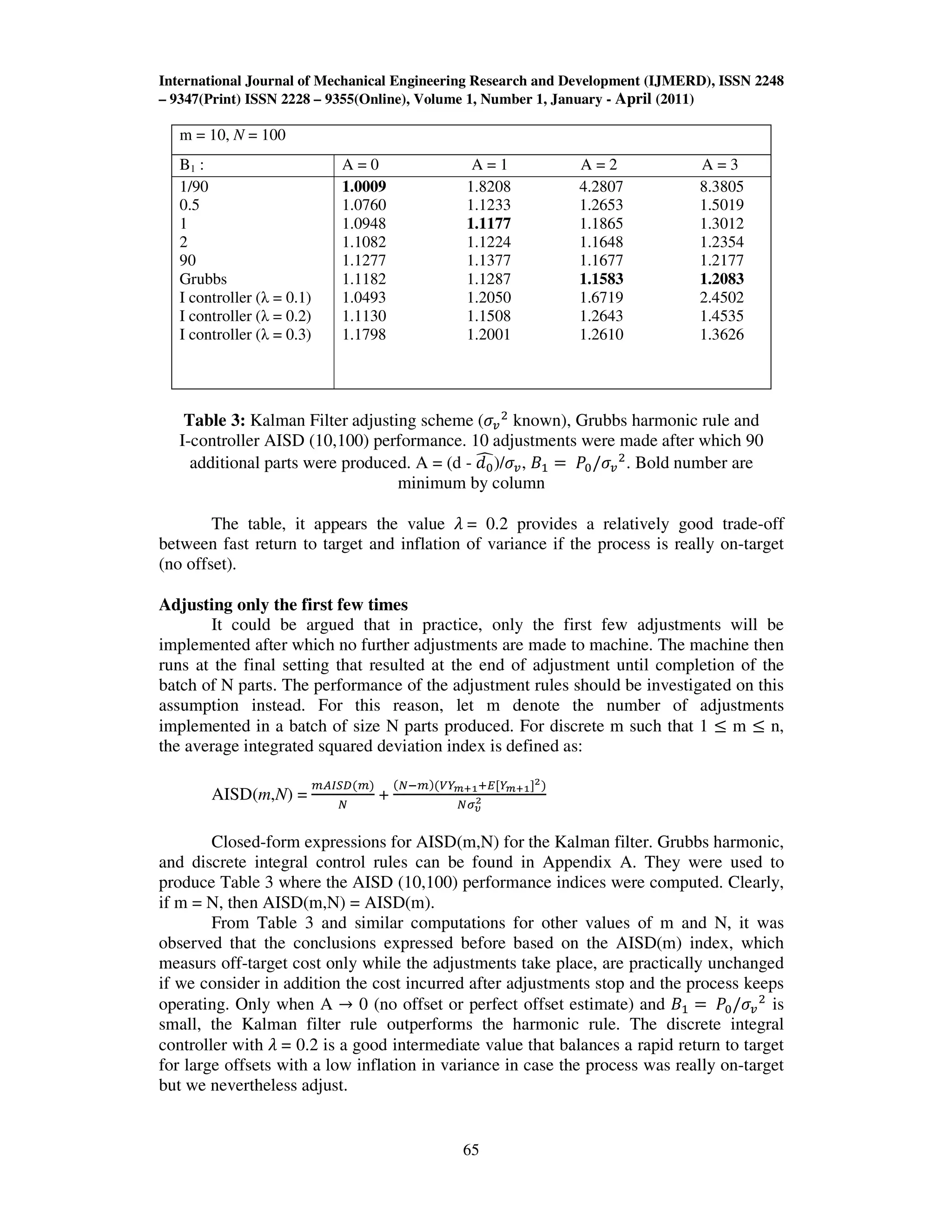
m = 10, N = 100
B1 : A = 0 A = 1 A = 2 A = 3
1/90
0.5
1
2
90
Grubbs
I controller (λ = 0.1)
I controller (λ = 0.2)
I controller (λ = 0.3)
1.0009 1.8208 4.2807 8.3805
1.0760 1.1233 1.2653 1.5019
1.0948 1.1177 1.1865 1.3012
1.1082 1.1224 1.1648 1.2354
1.1277 1.1377 1.1677 1.2177
1.1182 1.1287 1.1583 1.2083
1.0493 1.2050 1.6719 2.4502
1.1130 1.1508 1.2643 1.4535
1.1798 1.2001 1.2610 1.3626
Table 3: Kalman Filter adjusting scheme (ߪ௩
ଶ
known), Grubbs harmonic rule and
I-controller AISD (10,100) performance. 10 adjustments were made after which 90
additional parts were produced. A = (d - ݀଴
෢)/ߪ௩, ‫ܤ‬ଵ ൌ ܲ଴/ߪ௩
ଶ
. Bold number are
minimum by column
The table, it appears the value ߣ = 0.2 provides a relatively good trade-off
between fast return to target and inflation of variance if the process is really on-target
(no offset).
Adjusting only the first few times
It could be argued that in practice, only the first few adjustments will be
implemented after which no further adjustments are made to machine. The machine then
runs at the final setting that resulted at the end of adjustment until completion of the
batch of N parts. The performance of the adjustment rules should be investigated on this
assumption instead. For this reason, let m denote the number of adjustments
implemented in a batch of size N parts produced. For discrete m such that 1 ൑ m ൑ n,
the average integrated squared deviation index is defined as:
AISD(m,N) =
௠஺ூௌ஽ሺ௠ሻ
ே
+
ሺேି௠ሻሺ௏௒೘శభାாሾ௒೘శభሿమሻ
ேఙഔ
మ
Closed-form expressions for AISD(m,N) for the Kalman filter. Grubbs harmonic,
and discrete integral control rules can be found in Appendix A. They were used to
produce Table 3 where the AISD (10,100) performance indices were computed. Clearly,
if m = N, then AISD(m,N) = AISD(m).
From Table 3 and similar computations for other values of m and N, it was
observed that the conclusions expressed before based on the AISD(m) index, which
measurs off-target cost only while the adjustments take place, are practically unchanged
if we consider in addition the cost incurred after adjustments stop and the process keeps
operating. Only when A ՜ 0 (no offset or perfect offset estimate) and ‫ܤ‬ଵ ൌ ܲ଴/ߪ௩
ଶ
is
small, the Kalman filter rule outperforms the harmonic rule. The discrete integral
controller with ߣ = 0.2 is a good intermediate value that balances a rapid return to target
for large offsets with a low inflation in variance in case the process was really on-target
but we nevertheless adjust.
International Journal of Mechanical Engineering Research and Development (IJMERD), ISSN 2248
– 9347(Print) ISSN 2228 – 9355(Online), Volume 1, Number 1, January - April (2011)
66
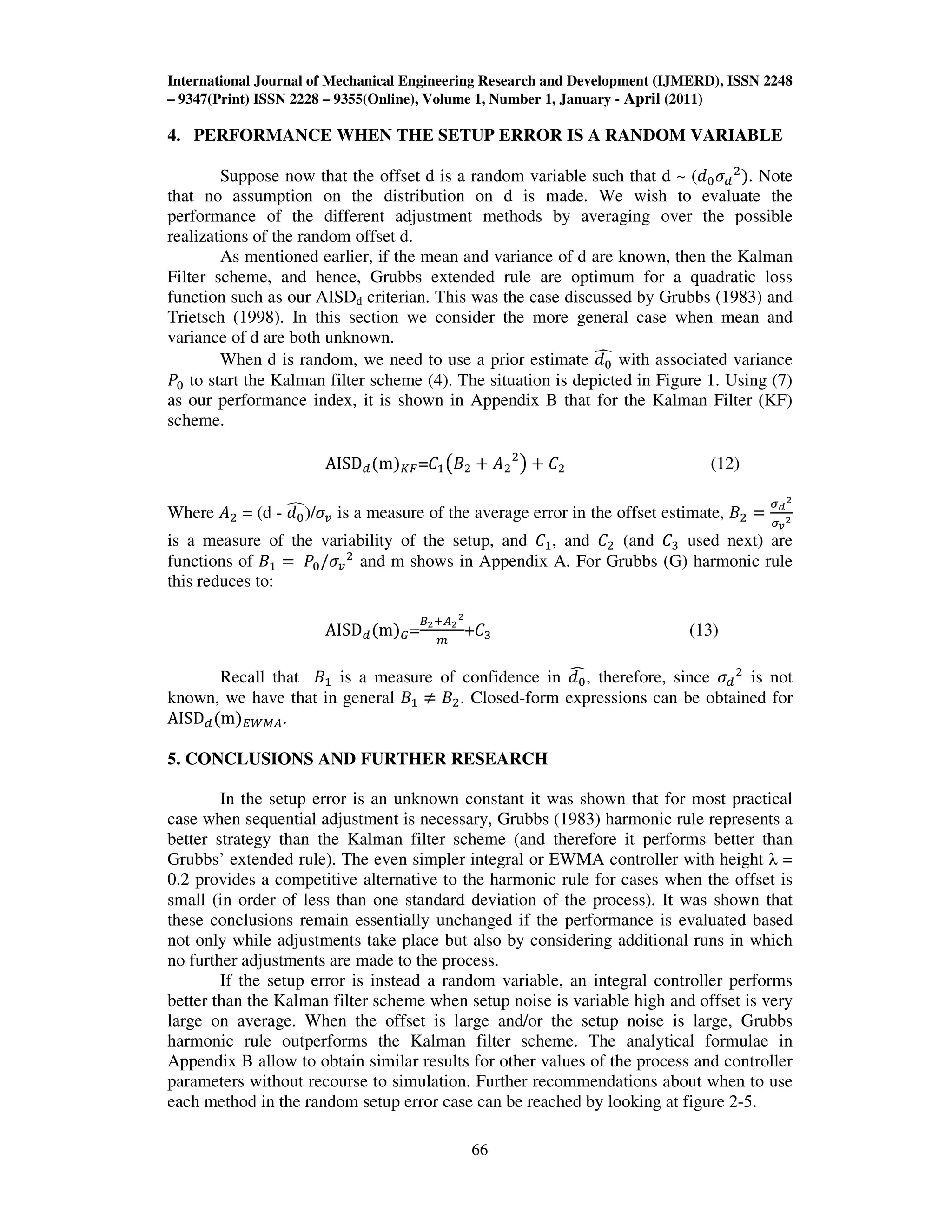
4. PERFORMANCE WHEN THE SETUP ERROR IS A RANDOM VARIABLE
Suppose now that the offset d is a random variable such that d ~ (݀଴ߪௗ
ଶ
ሻ. Note
that no assumption on the distribution on d is made. We wish to evaluate the
performance of the different adjustment methods by averaging over the possible
realizations of the random offset d.
As mentioned earlier, if the mean and variance of d are known, then the Kalman
Filter scheme, and hence, Grubbs extended rule are optimum for a quadratic loss
function such as our AISDd criterian. This was the case discussed by Grubbs (1983) and
Trietsch (1998). In this section we consider the more general case when mean and
variance of d are both unknown.
When d is random, we need to use a prior estimate ݀଴
෢ with associated variance
ܲ଴ to start the Kalman filter scheme (4). The situation is depicted in Figure 1. Using (7)
as our performance index, it is shown in Appendix B that for the Kalman Filter (KF)
scheme.
AISDௗሺmሻ௄ி=‫ܥ‬ଵ൫‫ܤ‬ଶ ൅ ‫ܣ‬ଶ
ଶ
൯ ൅ ‫ܥ‬ଶ (12)
Where ‫ܣ‬ଶ = (d - ݀଴
෢)/ߪ௩ is a measure of the average error in the offset estimate, ‫ܤ‬ଶ ൌ
ఙ೏
మ
ఙೡ
మ
is a measure of the variability of the setup, and ‫ܥ‬ଵ, and ‫ܥ‬ଶ (and ‫ܥ‬ଷ used next) are
functions of ‫ܤ‬ଵ ൌ ܲ଴/ߪ௩
ଶ
and m shows in Appendix A. For Grubbs (G) harmonic rule
this reduces to:
AISDௗሺmሻீ=
஻మା஺మ
మ
௠
+‫ܥ‬ଷ (13)
Recall that ‫ܤ‬ଵ is a measure of confidence in ݀଴
෢, therefore, since ߪௗ
ଶ
is not
known, we have that in general ‫ܤ‬ଵ ് ‫ܤ‬ଶ. Closed-form expressions can be obtained for
AISDௗሺmሻாௐெ஺.
5. CONCLUSIONS AND FURTHER RESEARCH
In the setup error is an unknown constant it was shown that for most practical
case when sequential adjustment is necessary, Grubbs (1983) harmonic rule represents a
better strategy than the Kalman filter scheme (and therefore it performs better than
Grubbs’ extended rule). The even simpler integral or EWMA controller with height λ =
0.2 provides a competitive alternative to the harmonic rule for cases when the offset is
small (in order of less than one standard deviation of the process). It was shown that
these conclusions remain essentially unchanged if the performance is evaluated based
not only while adjustments take place but also by considering additional runs in which
no further adjustments are made to the process.
If the setup error is instead a random variable, an integral controller performs
better than the Kalman filter scheme when setup noise is variable high and offset is very
large on average. When the offset is large and/or the setup noise is large, Grubbs
harmonic rule outperforms the Kalman filter scheme. The analytical formulae in
Appendix B allow to obtain similar results for other values of the process and controller
parameters without recourse to simulation. Further recommendations about when to use
each method in the random setup error case can be reached by looking at figure 2-5.
International Journal of Mechanical Engineering Research and Development (IJMERD), ISSN 2248
– 9347(Print) ISSN 2228 – 9355(Online), Volume 1, Number 1, January - April (2011)
67
The main advantage of the discrete integral controller over the other methods
considered in this paper is that it stays alert for compensating for further shifts in this
process that occur while manufacturing (i.e. not at setup). The weights in Grubbs rule,
for example, would have to be reset every time a shift is detected. This points toward
integration of the adjustment schemes with a detection mechanisms that will trigger the
adaptation of the weights, along the lines recently followed by Guo et al. (2000). Such
integrated SPC/EPC approaches require further research. The important connection
between Grubbs harmonic rule and Robbins and Monro’s stochastic Approximation
method (1951) point out to a very large body of literature and theoretical results some of
which may prove useful in process adjustment applications.
REFERENCES
1. Box, G.E.P., Luceno A (1997). Statistical control by monitoring and Feedback
Adjustment. John Wiley & Sons, New York, NY.
2. Del Castillo, E. (2001), “Some properties of EWMA feedback quality adjustment
schemes for drifting disturbances”, Journal of Quality Technology, 33(2), 153-166.
3. Del Castillo, E., Pan, Rong and Colosimo B. M. (2002). “An Unifying view of
Some Process Adjustment Methods”. Submitted for publication. Technical Paper,
Applied Statistical Laboratory, Department of Industrial Engineering, Penn State
University.
4. Grubbs, F.E., (1983). “An Optimum Procedure for Setting machines or
Adjusting Processes,” Journal of Quality Technology, 15, 4, pp. 186-189.
5. Guo R. S., Chen, A., and Chen, J. J., (2000). “An Enhance EWMA Controller for
Processes Subjected to Random Disturbances”, in Moyne, J., Del Castillo, E.,
and Hurwitz, A., Run to run control in semiconductor manufacturing, CRC press.
6. Robbins, H. and Monro, S. (1951). “A Stochastic Approximation Method”.
Annals of Mathematical Statistics, 22, pp. 400-407.
7. Trietsch, D., (1998). “The Harmonic Rule for Process setup Adjustment with
Quadratic Loss”, Journal of Quality Technology, 30, 1, pp. 75-84.

Study the different

  • 1.
    International Journal ofMechanical Engineering Research and Development (IJMERD), ISSN 2248 – 9347(Print) ISSN 2228 – 9355(Online), Volume 1, Number 1, January - April (2011) 60 STUDY THE DIFFERENT FEEDBACK METHODS IN MANUFACTURING SETUP ERRORS FOR CONSTANT AND RANDOM VARIABLES S Y Gajjal Dr. M D Jaybhaye Dr. A P S Gaur Asst. Prof.SCOE, Pune Asso. Prof.,COE, Pune Prof. BU, Jhansi ABSTRACT The performance criteria is the quadratic off-target cost incurred over a small number of parts produced. Analytical formulae are presented and numerically illustrated. Two cases are considered, the first one where the setup error is constant but unknown offset and the second one where the setup error is a random variable with unknown first two moments. It is shown how Grubbs’ harmonic rule and a simple integral provide a robust adjustment strategy in a variety of circumstances. As a by-product, the formulae presented in this paper allow to compute the expected off-target quadratic cost when a sudden shift occurs during production (not necessarily at setup) and the adjustment scheme compensates immediately after its occurrence. 1. INTRODUCTION Suppose that due to a defective setup machine operation, the quality characteristic generated by a production process is in state of statistical control but the process starts off-target. Adjusting the process is justified if the only relevant cost is the cost of running the process off-target. Sequential adjustment rules for this problem were proposed by Grubbs (1983). These rules have been shown to derive from much broader class of setup adjustment problems based on stochastic control methods by Del Castillo, Pan and Colosimo (2002). In this paper, the small sample performance of Grubbs adjustment rules are studied and contrasted with other feedback adjustment methods. To introduce some basic notation that will be based in that follows, let Yt denote the observed derivation from target of some quality characteristic of interest, following Grubbs (1983), a simple but useful model for the setup adjustment problem is to assume Yt = d+Ut-1+υt = µt + υt (1) Where d is the setup error, Ut is the level of controllable factor set after producing part t (this will have an immediate effect on part t+1), µt is the main deviation from target for part t, and υt ~ N (0,ߪజ ଶ ) models both the part-to-part variability and the measurement error. IJMERD © PRJ PUBLICATION International Journal of Mechanical Engineering Research and Development (IJMERD), ISSN 2248 – 9347(Print) ISSN 2228 – 9355(Online), Volume 1, Number 1 January - April (2011), pp. 60-67 © PRJ Publication, http://www.prjpublication.com/IJMERD.asp
  • 2.
    International Journal ofMechanical Engineering Research and Development (IJMERD), ISSN 2248 – 9347(Print) ISSN 2228 – 9355(Online), Volume 1, Number 1, January - April (2011) 61 Two different control rules were derived by Grubbs depending on two sets of assumptions made on setup error d: 1. If d is an unknown constant, minimization of Var(µn+1 ) subject to E [µn+1]=0 results in Grubbs’ “harmonic rule” :Ut = -݀መt, ݀መt=݀መt-1+KtYt (2) Kt = 1/t Or Ut - Ut-1 = ▽Ut =- ௒୲ ୲ Thus the weights Kt follow a harmonic series. An initial (a priori) estimate ݀መ0 is required to set the first setting of the controllable factor at U0 = -݀መ0. Del Castillo, Pan and Colosimo (2002) point out how adjustment rules (2) is a particular case of Robbins and Monro’s (1951) celebrated stochastic approximation method. Therefore, this paper contains (indirectly) a small-sample performance study of stochastic approximation methods applied to the simple case of estimation of an unknown constant. 2. If d ~ N (݀ҧ,ߪజ ଶ ) the both ݀ҧ and ߪௗ ଶ known, minimization of E [Σ௧ୀଵ ௡ ߤ௧ ଶ ] is achieved by Grubbs second adjustment rule. In this case, 3. ݀መt = ݀መt-1 + KtYt , Kt = ଵ ௧ା ഑ഔ మ ഑೏ మ and ▽Ut= - KtYt (3) This rule is called Grubbs’ “extended” rule by Trietsch (1998). Kt = ଵ ௧ା ഑ഔ మ ഑೏ మ , and ▽Ut= - KtYt (4) The interpretation is that, a priori, d ~ (݀መ0, P0). Thus for Grubbs’ extended rule to be optimal with respect to E [Σ௧ୀଵ ௡ ߤ௧ ଶ ] we need to know ݀ҧ (so we can set ݀ҧ0 = ݀ҧ) and ߪௗ ଶ and ߪజ ଶ must be known for us to use (3). Evidently, if P0 = ߪௗ ଶ , (3) and (4) are identical. Note how under this interpretation, if there is no prior information on offset (P0 → ∞) is equivalent to (2), Grubbs’ simpler harmonic rule. An additional adjustment rule that will be contrasted is an integral controller (Box and Luceno 1997); ▽Ut= - λYt (5) Which, contrary to Grubbs’ rules, does not converge to zero since λ is a constant.
  • 3.
    International Journal ofMechanical Engineering Research and Development (IJMERD), ISSN 2248 – 9347(Print) ISSN 2228 – 9355(Online), Volume 1, Number 1, January - April (2011) 62 2. PERFORMANCE INDICES FOR SS The Performance indices that will be used in the reminder of this paper are presented in this section for the two cases considered by Grubbs. Consider first the case where the setup error d is an unknown constant or “offset”. For this case, performance index considered is the scaled Average Integrated Square Deviation (AISD) incurred over m time instants or parts. This is defined for integer m > 0 as: ሺAISDሺ݉ሻሻ ൌ ଵ ௠ఙഔ మ ∑ ‫ܧ‬ሾܻ୧ ଶሿ ൌ௠ ௜ୀଵ ଵ ௠ఙഔ మ ∑ ሺVሾ௠ ௜ୀଵ ܻ௜ሿ ‫ܧ‬ሾܻ୧ ଶ ሿሻ ሺ6ሻ The AISD is a common performance index in the control engineering literature. Since Yi models deviations from target, the AISD index is like average “variance plus squared bias” calculation, and a surrogate of a quadratic off-target “loss” function. We avoid dependency on ߪజ ଶ by dividing by this quantity. ൫‫ܦܵܫܣ‬ௗሺ݉ሻ൯ ൌ ଵ ௠ఙഔ మ ‫ܧ‬ௗ ∑ ‫ܧ‬ሾܻ୧ ଶ ሿ ൌ௠ ௜ୀଵ ଵ ௠ఙഔ మ ‫׬‬ ∑ ‫ܧ‬ሾܻ୧ ଶ ሿ௠ ௜ୀଵ ∞ ି∞ ݂ௗሺ‫ݔ‬ሻ݀‫ݔ‬ ሺ7ሻ Where the outer expectation is taken over the distribution of d. note that if d is a non-random constant, then AISD(m) = AISDd(m). The case when d is normal with known mean and known variance was discussed by Trietsch (1998). Under such conditions, Gribbs’ extended rule is optimal for the AISDd criterian. 3. PERFORMANCE FOR AN UNKNOWN CONSTANT SETUP ERROR. Suppose d is an unknown constant but unaware of this fact a user applies Grubbs’ extended rule (i.e. the Kalman filter adjustment scheme given by (4)) To the process. It is shown in appendix A that this rule applied to the process Yt = d+Ut-1+υt (with d constant) results in ‫ܧ‬ሾܻtሿ ሺߪజሻ ൌ ‫ܣ‬ ‫ܤ‬ଵሺ‫ݐ‬ െ 1ሻ ൅ 1 ሺ8ሻ And ൌ 1 ௧ିଵ ቀሺ భ ಳభ ା௧ିଵሻమቁ ሺ9ሻ Where, ‫ܣ‬ ൌ ሺ݀ െ ݀଴ ෢ሻ/ߪ௩ measures how far off the initial estimate of the offset was. The quantity ‫ܤ‬ଵ ൌ ܲ଴/ߪ௩ ଶ is a measure of the “confidence” on the initial offset estimate. To study the performance of Grubbs adjustment rules, equations (8) and (9) can be substituted into equation (6) and the sum computed for given values of A, ‫ܤ‬ଵ and m. Note that our analytic expressions are exact and avoid use of simulation to estimate the AISD(m). Alternatively, an expression for the sum in AISD(m) is given by formula (17) in Appendix A which can be easier to use if a software that computes the polygamma
  • 4.
    International Journal ofMechanical Engineering Research and Development (IJMERD), ISSN 2248 – 9347(Print) ISSN 2228 – 9355(Online), Volume 1, Number 1, January - April (2011) 63 function is available (e.g., Mathematica or Maple). We note that the corresponding expressions for Grubbs harmonic rule are obtained from (8) and (9) by letting ‫ܤ‬ଵ ՜ ∞. For a discrete integral controller (or EWMA controller), it can be shown that ‫ܧ‬ሾܻtሿ ሺߪజሻ ൌ ሺሺ1 െ λሻ௧ିଵ ‫ܣ‬ሻ ሺ10ሻ and ௏ሾ௒୲ሿ ఙഔ మ ൌ ଶିλሺଵିλሻమሺ೟షభሻ ଶିλ ሺ11ሻ From where AISD(m) = ଵ ௠ఙೡ మ ∑ ሺ‫ܧ‬ሾܻ௜ሿଶ௠ ௜ୀଵ ൅ ܸሾܻ௜ሿሻ can be computed or one can use the closed-form expression (eq. 18) in Appendix A. The AISD(m) expressions allow to study the trade-offs between the sum of the variances and the sum of squared expected deviations (squared bias). For the kalman filter scheme, as ‫ܤ‬ଵ ൌ ܲ଴/ߪ௩ ଶ ՜ 0, implying increasingly higher confidence in the priori offset estimate, then ݉ଵ ∑ ሺܸሾܻ௜ሿ/ߪ௩ ଶ ሻ௠ ௜ ୀ ଵ ՜ 1 (i.e., we get lower variance), but ݉ଵ ∑ ሺ‫ܧ‬ሾܻ௜ሿ/ߪ௩ ଶ ሻ௠ ௜ ୀ ଵ ՜ ‫ܣ‬ଶ (i.e., we get larger bias). Similarly, for the EWMA or integral controller, as ߣ ՜ 0, implying less weight given to the last observation we have ݉ଵ ∑ ሺܸሾܻ௜ሿ/ߪ௩ ଶ ሻ௠ ௜ ୀ ଵ ՜ 1 (lower variance), but ݉ଵ ∑ ሺ‫ܧ‬ሾܻ௜ሿ/ߪ௩ ଶ ሻ௠ ௜ ୀ ଵ ՜ ‫ܣ‬ଶ (larger bias). There are two parameters that can be modified in Grubbs adjustment rules: ݀଴ ෢ and ܲ଴. The effect of these parameters can be studied from looking at the effect of changes in A and ‫ܤ‬ଵ, as previously defined. Therefore, the four scenarios presented in Table 1 were investigated. ‫ܤ‬ଵ small ‫ܤ‬ଵ large |‫|ܣ‬ small Good choice (case 1) Bad choice (case 2) |‫|ܣ‬ large Bad choice (case 3) Good choice (4) Table 1: Scenarios of interest, adjusting schemes, A = (d - ݀଴ ෢)/ߪ௩, ‫ܤ‬ଵ ൌ ܲ଴/ߪ௩ ଶ In the table, if the initial prior variance ܲ଴ is large relative to ߪ௩ ଶ (i.e., if ‫ܤ‬ଵ is large), the weights ‫ܭ‬௧ will be close to 1/t (Grubbs harmonic rule), i.e., the initial estimate ݀଴ ෢ will be discounted faster. This turns out to be a good decision if the initial offset estimate is far from d, where the distance between d and ݀଴ ෢ is measured relative to ߪ௩. A similar good decision is when ܲ଴ is low and ݀଴ ෢ is a good estimate of offset (‫ܤ‬ଵ small, |‫|ܣ‬ small). In such case, ‫ܭ‬௧ ൏ 1/t, so there will be slower discounting of the initial estimate ݀଴ ෢. Cases (2) and (3) on the table indicate bad decisions, when the value of ܲ଴ does not reflet how good the initial offset estimate really is. Since in the absence of historical information it is difficult to know a priori the value of practical interest to study the four cases on the Table. Table 2 contrast the AISD performance of Grubbs harmonic rule, the discrete integral controller (EWMA controller) and the kalman filter adjusting scheme (ߪ௩ ଶ known). The table shows the values of AISD(m) for m = 5,10 and 20. As can be seen from the Table, the “gap” between the column minimum and the AISD provided by Grubbs rule shrinks as the offset d gets much larger than ߪ௩ (i.e., as |‫|ܣ‬ increases). This gap, however, is quite moderate except in the case where one is very confident
  • 5.
    International Journal ofMechanical Engineering Research and Development (IJMERD), ISSN 2248 – 9347(Print) ISSN 2228 – 9355(Online), Volume 1, Number 1, January - April (2011) 64 (‫ܤ‬ଵ ൌ ܲ଴/ߪ௩ ଶ small) of our a priori offset estimate turns out to be quite accurate (i.e., A = 0). This is not a practical case because it implies we practically know the value of the offset d. m = 5 B1 : |A| = 0 |A| = 1 |A| = 2 |A| = 3 1/90 0.5 1 2 90 Grubbs I controller (λ = 0.1) I controller (λ = 0.2) I controller (λ = 0.3) 1.00023 1.95791 4.83092 9.61929 1.09344 1.48656 5.66589 4.63144 1.16394 1.45667 5.33486 3.79844 1.24138 1.47815 2.1884 7 3.37233 1.41043 1.61046 2.21056 3.21074 1.41667 1.61667 2.21667 3.21667 1.01655 1.70215 3.75895 7.18696 1.05601 1.55191 3.03962 5.51914 1.10922 1.49030 2.63354 4.53894 m = 10 B1 : |A| = 0 |A| = 1 |A| = 2 |A| = 3 1/90 0.5 1 2 90 Grubbs I controller (λ = 0.1) I controller (λ = 0.2) I controller (λ = 0.3) 1.00049 1.91004 4.63869 9.18644 1.09038 1.31359 1.98323 3.09930 1.13792 1.29290 1.75783 2.53271 1.18491 1.30578 1.66840 2.27276 1.27952 1.37954 1.67959 2.17969 1.28290 1.38290 1.68290 2.18290 1.02830 1.49063 2.87761 5.18925 1.08060 1.35518 2.17890 3.55178 1.14190 1.33782 1.92558 2.90518 m = 20 B1 : |A| = 0 |A| = 1 |A| = 2 |A| = 3 1/90 0.5 1 2 90 Grubbs I controller (λ = 0.1) I controller (λ = 0.2) I controller (λ = 0.3) 1.00090 1.82739 4.30685 8.43929 1.07243 1.19211 1.55117 2.14960 1.10008 1.17989 1.41931 1.81895 1.12585 1.18691 1.37009 1.67539 1.17564 1.22565 1.37568 1.62573 1.17739 1.22739 1.37739 1.62739 1.03899 1.29825 2.07606 3.37240 1.09568 1.23455 1.65116 2.34552 1.15917 1.25721 1.55133 2.04152 Table 2: Kalman Filter adjusting scheme (ߪ௩ ଶ known), Grubbs harmonic rule and Integral controller AISD performance. A = (d - ݀଴ ෢)/ߪ௩, ‫ܤ‬ଵ ൌ ܲ଴/ߪ௩ ଶ . Bold number are minimum by column
  • 6.
    International Journal ofMechanical Engineering Research and Development (IJMERD), ISSN 2248 – 9347(Print) ISSN 2228 – 9355(Online), Volume 1, Number 1, January - April (2011) 65 m = 10, N = 100 B1 : A = 0 A = 1 A = 2 A = 3 1/90 0.5 1 2 90 Grubbs I controller (λ = 0.1) I controller (λ = 0.2) I controller (λ = 0.3) 1.0009 1.8208 4.2807 8.3805 1.0760 1.1233 1.2653 1.5019 1.0948 1.1177 1.1865 1.3012 1.1082 1.1224 1.1648 1.2354 1.1277 1.1377 1.1677 1.2177 1.1182 1.1287 1.1583 1.2083 1.0493 1.2050 1.6719 2.4502 1.1130 1.1508 1.2643 1.4535 1.1798 1.2001 1.2610 1.3626 Table 3: Kalman Filter adjusting scheme (ߪ௩ ଶ known), Grubbs harmonic rule and I-controller AISD (10,100) performance. 10 adjustments were made after which 90 additional parts were produced. A = (d - ݀଴ ෢)/ߪ௩, ‫ܤ‬ଵ ൌ ܲ଴/ߪ௩ ଶ . Bold number are minimum by column The table, it appears the value ߣ = 0.2 provides a relatively good trade-off between fast return to target and inflation of variance if the process is really on-target (no offset). Adjusting only the first few times It could be argued that in practice, only the first few adjustments will be implemented after which no further adjustments are made to machine. The machine then runs at the final setting that resulted at the end of adjustment until completion of the batch of N parts. The performance of the adjustment rules should be investigated on this assumption instead. For this reason, let m denote the number of adjustments implemented in a batch of size N parts produced. For discrete m such that 1 ൑ m ൑ n, the average integrated squared deviation index is defined as: AISD(m,N) = ௠஺ூௌ஽ሺ௠ሻ ே + ሺேି௠ሻሺ௏௒೘శభାாሾ௒೘శభሿమሻ ேఙഔ మ Closed-form expressions for AISD(m,N) for the Kalman filter. Grubbs harmonic, and discrete integral control rules can be found in Appendix A. They were used to produce Table 3 where the AISD (10,100) performance indices were computed. Clearly, if m = N, then AISD(m,N) = AISD(m). From Table 3 and similar computations for other values of m and N, it was observed that the conclusions expressed before based on the AISD(m) index, which measurs off-target cost only while the adjustments take place, are practically unchanged if we consider in addition the cost incurred after adjustments stop and the process keeps operating. Only when A ՜ 0 (no offset or perfect offset estimate) and ‫ܤ‬ଵ ൌ ܲ଴/ߪ௩ ଶ is small, the Kalman filter rule outperforms the harmonic rule. The discrete integral controller with ߣ = 0.2 is a good intermediate value that balances a rapid return to target for large offsets with a low inflation in variance in case the process was really on-target but we nevertheless adjust.
  • 7.
    International Journal ofMechanical Engineering Research and Development (IJMERD), ISSN 2248 – 9347(Print) ISSN 2228 – 9355(Online), Volume 1, Number 1, January - April (2011) 66 4. PERFORMANCE WHEN THE SETUP ERROR IS A RANDOM VARIABLE Suppose now that the offset d is a random variable such that d ~ (݀଴ߪௗ ଶ ሻ. Note that no assumption on the distribution on d is made. We wish to evaluate the performance of the different adjustment methods by averaging over the possible realizations of the random offset d. As mentioned earlier, if the mean and variance of d are known, then the Kalman Filter scheme, and hence, Grubbs extended rule are optimum for a quadratic loss function such as our AISDd criterian. This was the case discussed by Grubbs (1983) and Trietsch (1998). In this section we consider the more general case when mean and variance of d are both unknown. When d is random, we need to use a prior estimate ݀଴ ෢ with associated variance ܲ଴ to start the Kalman filter scheme (4). The situation is depicted in Figure 1. Using (7) as our performance index, it is shown in Appendix B that for the Kalman Filter (KF) scheme. AISDௗሺmሻ௄ி=‫ܥ‬ଵ൫‫ܤ‬ଶ ൅ ‫ܣ‬ଶ ଶ ൯ ൅ ‫ܥ‬ଶ (12) Where ‫ܣ‬ଶ = (d - ݀଴ ෢)/ߪ௩ is a measure of the average error in the offset estimate, ‫ܤ‬ଶ ൌ ఙ೏ మ ఙೡ మ is a measure of the variability of the setup, and ‫ܥ‬ଵ, and ‫ܥ‬ଶ (and ‫ܥ‬ଷ used next) are functions of ‫ܤ‬ଵ ൌ ܲ଴/ߪ௩ ଶ and m shows in Appendix A. For Grubbs (G) harmonic rule this reduces to: AISDௗሺmሻீ= ஻మା஺మ మ ௠ +‫ܥ‬ଷ (13) Recall that ‫ܤ‬ଵ is a measure of confidence in ݀଴ ෢, therefore, since ߪௗ ଶ is not known, we have that in general ‫ܤ‬ଵ ് ‫ܤ‬ଶ. Closed-form expressions can be obtained for AISDௗሺmሻாௐெ஺. 5. CONCLUSIONS AND FURTHER RESEARCH In the setup error is an unknown constant it was shown that for most practical case when sequential adjustment is necessary, Grubbs (1983) harmonic rule represents a better strategy than the Kalman filter scheme (and therefore it performs better than Grubbs’ extended rule). The even simpler integral or EWMA controller with height λ = 0.2 provides a competitive alternative to the harmonic rule for cases when the offset is small (in order of less than one standard deviation of the process). It was shown that these conclusions remain essentially unchanged if the performance is evaluated based not only while adjustments take place but also by considering additional runs in which no further adjustments are made to the process. If the setup error is instead a random variable, an integral controller performs better than the Kalman filter scheme when setup noise is variable high and offset is very large on average. When the offset is large and/or the setup noise is large, Grubbs harmonic rule outperforms the Kalman filter scheme. The analytical formulae in Appendix B allow to obtain similar results for other values of the process and controller parameters without recourse to simulation. Further recommendations about when to use each method in the random setup error case can be reached by looking at figure 2-5.
  • 8.
    International Journal ofMechanical Engineering Research and Development (IJMERD), ISSN 2248 – 9347(Print) ISSN 2228 – 9355(Online), Volume 1, Number 1, January - April (2011) 67 The main advantage of the discrete integral controller over the other methods considered in this paper is that it stays alert for compensating for further shifts in this process that occur while manufacturing (i.e. not at setup). The weights in Grubbs rule, for example, would have to be reset every time a shift is detected. This points toward integration of the adjustment schemes with a detection mechanisms that will trigger the adaptation of the weights, along the lines recently followed by Guo et al. (2000). Such integrated SPC/EPC approaches require further research. The important connection between Grubbs harmonic rule and Robbins and Monro’s stochastic Approximation method (1951) point out to a very large body of literature and theoretical results some of which may prove useful in process adjustment applications. REFERENCES 1. Box, G.E.P., Luceno A (1997). Statistical control by monitoring and Feedback Adjustment. John Wiley & Sons, New York, NY. 2. Del Castillo, E. (2001), “Some properties of EWMA feedback quality adjustment schemes for drifting disturbances”, Journal of Quality Technology, 33(2), 153-166. 3. Del Castillo, E., Pan, Rong and Colosimo B. M. (2002). “An Unifying view of Some Process Adjustment Methods”. Submitted for publication. Technical Paper, Applied Statistical Laboratory, Department of Industrial Engineering, Penn State University. 4. Grubbs, F.E., (1983). “An Optimum Procedure for Setting machines or Adjusting Processes,” Journal of Quality Technology, 15, 4, pp. 186-189. 5. Guo R. S., Chen, A., and Chen, J. J., (2000). “An Enhance EWMA Controller for Processes Subjected to Random Disturbances”, in Moyne, J., Del Castillo, E., and Hurwitz, A., Run to run control in semiconductor manufacturing, CRC press. 6. Robbins, H. and Monro, S. (1951). “A Stochastic Approximation Method”. Annals of Mathematical Statistics, 22, pp. 400-407. 7. Trietsch, D., (1998). “The Harmonic Rule for Process setup Adjustment with Quadratic Loss”, Journal of Quality Technology, 30, 1, pp. 75-84.