This paper presents a robust adaptive type-2 fuzzy second-order sliding mode controller designed for stabilizing uncertain chaotic systems affected by internal parameter uncertainties and external disturbances. The control strategy reduces chattering using a super twisting algorithm, integrating adaptive interval type-2 fuzzy systems to approximate system dynamics and derive stability guarantees. An illustrative example demonstrates the effectiveness of the proposed controller in achieving desired system behavior.

1. International Journal of Computational Science, Information Technology and Control Engineering (IJCSITCE) Vol.2, No.4, October 2015
DOI : 10.5121/ijcsitce.2015.2401 1
ADAPTIVE TYPE-2 FUZZY SECOND ORDER SLIDING
MODE CONTROL FOR NONLINEAR UNCERTAIN
CHAOTIC SYSTEM
Rim Hendel1
, Farid Khaber1
and Najib Essounbouli2
1
QUERE Laboratory, Engineering Faculty, University of Setif 1, 19000 Setif, Algeria
2
CReSTIC of Reims Champagne-Ardenne University,IUT de Troyes, France
ABSTRACT
In this paper, a robust adaptive type-2 fuzzy nonsingular sliding mode controller is designed to stabilize the
unstable periodic orbits of uncertain perturbed chaotic system with internal parameter uncertainties and
external disturbances. In Higher Order Sliding Mode Control (HOSMC),the chattering phenomena of the
control effort is reduced, by using Super Twisting algorithm. Adaptive interval type-2 fuzzy systems are
proposed to approximate the unknown part of uncertain chaotic system and to generate the Super Twisting
signals. Based on Lyapunov criterion, adaptation laws are derived and the closed loop system stability is
guaranteed. An illustrative example is given to demonstrate the effectiveness of the proposed controller.
KEYWORDS
Chaotic System, Type-2 Fuzzy Logic System, second order Sliding Mode Control, Lyapunov Stability.
1. INTRODUCTION
Chaotic phenomenon is widely observed in several applications such as: medical field, fractal
theory, electrical circuits and secure communication [1]. Although, the prominent characteristics
of chaotic system is its extreme sensitivity to initial conditions and its unpredictability; it is
usually difficult to predict exactly the behavior of the chaotic system. Recently, several
researchers have focused on chaos control [2]. Many nonlinear control techniques have been
successfully applied on chaos control and synchronization of different dynamical systems [3-5],
nonlinear control [6-7], active control and backstepping design [8-10], fuzzy logic and adaptive
control [11-12], adaptive fuzzy control [13].
Unfortunately, in the most of the approaches mentioned above the unknown parameters of the
chaotic system,the uncertainties,internal and external disturbances, have not been considered,
which implies that the robustness has not been investigated. Sliding Mode Control (SMC) is often
adopted, due to its inherent advantages of fast dynamic response, guaranteed stability, robustness
against matching external disturbances, andinternal parameter variations. Several controllers
based on sliding mode control have been proposed for chaos schemes [14-16].
However, it should be noted that the smoothness of a control signal in sliding mode is not easily
achievable without loss performance and robustness degradation. A lot of works have been
proceeded to solve this problem by using adaptive control [17-18], and intelligent approaches
[19-20].
The High Order Sliding Mode Control (HOSMC) has been presented to reduce and (or) remove
the chattering phenomenon. Moreover, this technique provides higher accuracy than the
standardSMC [21-23]. Higher order sliding modes (HOSM) generalize the basic so-called first

2. International Journal of Computational Science, Information Technology and Control Engineering (IJCSITCE) Vol.2, No.4, October 2015
2
order sliding mode idea acting on the higher order time derivatives of sliding function. In the case
of second order sliding mode, the sliding set is described asS = {s = sሶ = 0, sሷ ≠ 0}, and the
control is acting on the second derivative of the switching manifold s [24-25]. A HOSMC has a
finite time convergence, which is satisfied when the switching gains in the HOSM control law are
selected properly. Nevertheless, the calculation of these gains needs the well knowledge of the
system dynamic [21,26].
In this paper, a higher order sliding mode controlcombined with adaptive type-2 fuzzy systems, is
proposed to design a robust controller for stabilization of unknown SISO nonlinear chaotic
system, working in the presence of uncertainties and external disturbances. The Super Twisting
algorithm is implemented to avoid a chattering phenomenon. In the same time, we introduced
adaptive type-2 fuzzy systems for model the unknown dynamic of system and simplify the
calculation of gains in the second order sliding mode. Their updates are performed using
adaptation laws derived from the stability studyin the Lyapunov sense.
The organization of this paper is as follows. In section 2, the problem states and description of the
system.The adaptive type-2 fuzzy second order sliding mode control scheme is presented in
section III. Simulation example demonstrate the efficiently of the proposed approach in section
IV. Finally, section V gives the conclusions of the advocated design methodology.
2. DESCRIPTION OF SYSTEM AND PROBLEM FORMULATION
Consider n-order uncertain chaotic system which has an affine form:
൜
‫ݔ‬ሶ݅ = ‫ݔ‬݅+1, 1 ≤ ݅ ≤ ݊ − 1,
‫ݔ‬ሶ݊ = ݂(‫,ݔ‬ ‫)ݐ‬ + Δ݂(‫,ݔ‬ ‫)ݐ‬ + ݀(‫)ݐ‬ + ‫)ݐ(ݑ‬ ,
(1)
where ‫ݔ‬ = [‫ݔ‬1(‫ݔ )ݐ‬2(‫… )ݐ‬ ‫ݔ‬݊(‫])ݐ‬ ∈ ℜ݊
is the measurable state vector, ݂(‫,ݔ‬ ‫)ݐ‬is unknown
nonlinear continuous and bounded function, ‫)ݐ(ݑ‬ ∈ ℜis control input of the system, Δ݂(‫,ݔ‬ ‫)ݐ‬and
݀(‫)ݐ‬are the uncertainties and external bounded disturbances, respectively,
ห݂(‫,ݔ‬ ‫)ݐ‬ห < ‫ , ܨ‬หΔ݂(‫,ݔ‬ ‫)ݐ‬ห ≤ Δ݂ , |݀(‫)ݐ‬| ≤ Δ݀ (2)
where‫ , ܨ‬Δ௙ and Δ݀ are positive constants.
The control objective is getting the system to track an n- dimensional desired vector ‫ݕ‬
݀
(‫)ݐ‬which
belong to a class of continuous functions on[‫ݐ‬଴, ∞]. Let’s the tracking error as;
݁(‫)ݐ‬ = ‫)ݐ(ݔ‬ − ‫ݕ‬
݀
(‫)ݐ‬
= [‫)ݐ(ݔ‬ − ‫ݕ‬݀
(‫ݔ )ݐ‬ሶ(‫)ݐ‬ − ‫ݕ‬ሶ݀
(‫ݔ … )ݐ‬(݊−1)
(‫)ݐ‬ − ‫ݕ‬݀
(݊−1)
(‫] )ݐ‬
= [݁(‫݁ )ݐ‬ሶ(‫. )ݐ‬ . . ݁(݊−1)
(‫])ݐ‬
(3)
Therefore, the dynamic errors of system can be obtained as;
‫ە‬
‫۔‬
‫ۓ‬
݁ሶ1 = ݁2
݁ሶ2 = ݁3,
⋮
݁ሶ݊ = ݂(‫,ݔ‬ ‫)ݐ‬ − ‫ݕ‬݀
(݊)
(‫)ݐ‬ + Δ݂(‫,ݔ‬ ‫)ݐ‬ + ݀(‫)ݐ‬ + ‫)ݐ(ݑ‬
(4)
The control goal considered is that;
lim
௧→ஶ
ቛ݁
ି
(‫)ݐ‬ቛ = lim
௧→ஶ
ฯ‫ݔ‬
ି
(‫)ݐ‬ − ‫ݕ‬
ି
ௗ(‫)ݐ‬ฯ → 0, (5)

3. International Journal of Computational Science, Information Technology and Control Engineering (IJCSITCE) Vol.2, No.4, October 2015
3
2.1. Second Order Sliding Mode Control
The basic concept of second order sliding mode control can be interpreted from the following the
following second order nonlinear system:
൜
‫ݔ‬ሶ1 = ‫ݔ‬2 ,
‫ݔ‬ሶ2 = ݂(‫,ݔ‬ ‫)ݐ‬ + ‫,ݔ(ܦ‬ ‫)ݐ‬ + ‫,)ݐ(ݑ‬
(6)
‫,ݔ(ܦ‬ ‫)ݐ‬isthe whole uncertainties indicating the sum of the external disturbances and parameter
uncertainties, where‫,ݔ(ܦ‬ ‫)ݐ‬ ≤ Δ and Δ = Δ௙ + Δௗ.
The linear sliding manifold is defined as,
‫,݁(ݏ‬ ‫)ݐ‬ = ቀ
ப
ப௧
+ ߣቁ
(௡ିଵ)
݁ (7)
whereλ > 0 is a positiveconstant, The time derivative of ‫ݏ‬ is:
‫ݏ‬ሶ(݁, ‫)ݐ‬ = ݁(݊)
+ ߜ‫ݏ‬
whereߜ‫ݏ‬ = ∑
(݊−1)!
݇!(݊−݇−1)!
݊
݇=1 ቀ
∂
∂‫ݐ‬
ቁ
(݊−݇−1)
ߣ݇
݁ሶ.
By using system (6) we obtain;
‫ݏ‬ሶ(݁, ‫)ݐ‬ = ߜ௦ + ‫ݕ‬ሷௗ − ݂(‫,ݔ‬ ‫)ݐ‬ − ‫)ݐ(ݑ‬ − ‫,ݔ(ܦ‬ ‫)ݐ‬ (8)
If ݂(‫,ݔ‬ ‫)ݐ‬ is known and free of external disturbancesanduncertainties, and when the system (6) is
restricted to the(݁
ି
, ‫)ݐ‬ = 0, it will be governed by an equivalent control ‫ݑ‬݁‫ݍ‬obtained by:
‫ݑ‬݁‫ݍ‬ = − ቂ݂(‫ݔ‬
−
, ‫)ݐ‬ − ‫ݕ‬ሷ݀
− δ‫ݏ‬ቃ (9)
The global control is composed of the equivalent control and the Super Twisting terms ‫ݑ‬ଵand
‫ݑ‬ଶsuch that;
ቊ
‫ݑ‬ሶଵ = −ߣଵ‫,݁(ݏ(݊݃݅ݏ‬ ‫))ݐ‬
‫ݑ‬ଶ = −ߣଶห‫,ݔ(ݏ‬ ‫)ݐ‬ห
(ଵ/ଶ)
‫,݁(ݏ(݊݃݅ݏ‬ ‫))ݐ‬
(10)
where ߣଵܽ݊݀ߣଶ, are the Super Twisting control gains [21], by adding these term to (9), we obtain
the global control:
‫ݑ‬ = − ቂ݂(‫ݔ‬
ି
, ‫)ݐ‬ − ‫ݕ‬ሷௗ − δ௦ − ‫׬‬ ‫ݑ‬ሶଵ
்
଴
− ‫ݑ‬ଶቃ (11)
The sufficient condition to ensure the transition trajectory of the tracking error from approaching
phase to the sliding one is:
1
2
݀
݀‫ݐ‬
‫ݏ‬2
(݁
−
, ‫)ݐ‬ = ‫݁(ݏ‬
−
, ‫ݏ)ݐ‬ሶ(݁
−
, ‫)ݐ‬ ≤ −η ቚ‫݁(ݏ‬
−
, ‫)ݐ‬ቚ (12)
whereη > 0is a constant.
After some manipulations, we obtain:

4. International Journal of Computational Science, Information Technology and Control Engineering (IJCSITCE) Vol.2, No.4, October 2015
4
−ߣଵ‫ݐ‬ − ߣଶห‫,݁(ݏ‬ ‫)ݐ‬ห
(ଵ/ଶ)
+ ‫,ݔ(ܦ‬ ‫݊݃݅ݏ )ݐ‬൫‫,݁(ݏ‬ ‫)ݐ‬൯ ≤ −ߟ (13)
Then we can choose the parameters of ߣ1 and ߣ2as follows:
ߣ1‫ݐ‬ + ߣ2ห‫,݁(ݏ‬ ‫)ݐ‬ห
(1/2)
≥ ߟ + ห‫,ݔ(ܦ‬ ‫)ݐ‬ห
≥ ߟ + Δ
(14)
Note that the control law (11) depends only on the parametersߣ , ߣଵ , ߣଶ, and nonlinear
continuous function݂(‫,ݔ‬ ‫. )ݐ‬ However, the knowledge of the ‫ݏ′ܦ‬ upper bound and݂(‫,ݔ‬ ‫ )ݐ‬ is
required in the optimal choice ofߣ1and ߣ2, in the approaching phase. Therefore ݂(‫,ݔ‬ ‫ )ݐ‬ is
unknown and(‫,ݔ‬ ‫)ݐ‬ ≠ 0.
In the rest of paper we solved these problems by introducing an adaptive fuzzy second order
sliding mode controller.
2.2. Interval Type-2 Fuzzy Logic System
Fuzzy Logic Systems (FLSs) are known as the universal approximators and have several
applications in control designandidentification. A type-1 fuzzy system consists of four major
parts: fuzzifier, rule base, inference engine, and defuzzifier. A T2FLS is very similar to a T1FLS
[27], the major structure difference being that the defuzzifier block of a T1FLS is replaced by the
output processing block in a T2FLS, which consists of type-reduction followed by
defuzzification.
Figure 1. Structure of a type-2 fuzzy logic system.
In a T2FS, a Gaussian function with a known standard deviation is chosen, while the mean (m)
varies between m1and m2. Therefore, a uniform weighting is assumed to represent a footprint of
uncertainty as shaded in Figure. 2.
Fuzzifier
Rule base
Inference engine
Type reducer
Defuzzifier
Crisp
Output y
Type
Reduced set
Fuzzy
Output sets
Fuzzy
Intput sets
Output
Type-2 fuzzy logic system
Crisp
Input

5. International Journal of Computational Science, Information Technology and Control Engineering (IJCSITCE) Vol.2, No.4, October 2015
5
Figure 2. Interval type-2 Gaussian fuzzy set.
It is clear that the type-2 fuzzy set is in a region bounded by an upper MF and a lower MF
denoted as ߤത‫ܣ‬෩(‫ݔ‬) and ߤ
‫ܣ‬෩
(‫ݔ‬) respectively, and is named a foot of uncertainty (FOU). Assume that
there are M rules in a type-2 fuzzy rule base, each of which has the following form:
ܴ݅
: ‫ݔܨܫ‬1݅‫ܨݏ‬෨1
݅
, ܽ݊݀ … , ܽ݊݀‫ݔ‬݊݅‫ܨݏ‬෨݊
݅
, ܶ‫ݏ݅ݕܰܧܪ‬[‫ݓ‬݈
݅
‫ݓ‬‫ݎ‬
݅ ]
wherexj, j=1,2,…,n and y are the input and output variables of the type-2 fuzzy system,
respectively, the ‫ܨ‬෨݊
݅
is the type-2 fuzzy sets of antecedent part, and [‫ݓ‬݈
݅
‫ݓ‬‫ݎ‬
݅ ] is the weighting
interval set in the consequent part. The operation of type-reduction is to give a type-1 set from a
type-2 set. In the meantime, the firing strength Fi
for the ith rule can be an interval type-2 set
expressed as;
‫ܨ‬݅
≡ [݂݅
, ݂
݅
] (15)
where
ቐ
݂݅
= ߤ
‫ܨ‬෩1
݅ (‫ݔ‬1) ∗ … ∗ ߤ
‫ܨ‬෩݊
݅ (‫ݔ‬݊)
݂
݅
= ߤ‫ܨ‬෩1
݅ (‫ݔ‬1) ∗ … ∗ ߤ‫ܨ‬෩݊
݅ (‫ݔ‬݊)
(16)
In this paper, the center of set type-reduction method is used to simplify the notation. Therefore,
the output can be expressed as;
‫ݕ‬cos
(‫)ݔ‬ = ൣ‫ݕ‬݈
, ‫ݕ‬‫ݎ‬
൧
= ‫׬‬‫ݓ‬1∈ൣ‫ݓ‬݈
1
,‫ݓ‬‫ݎ‬
1൧ … ‫׬‬‫ݓ‬‫ܯ‬∈ൣ‫ݓ‬݈
‫ܯ‬
,‫ݓ‬‫ݎ‬
‫ܯ‬൧ × ‫׬‬݂1
∈ቂ݂1
,݂ത1
ቃ
… ‫׬‬݂‫ܯ‬
∈ቂ݂‫ܯ‬
,݂ത‫ܯ‬
ቃ
1
∑ ݂݅
‫ݓ‬݅‫ܯ‬
݅=1
∑ ݂݅‫ܯ‬
݅=1
ൗ
(17)
where ‫ݕ‬cos
(‫)ݔ‬ is also an interval type-1 set determined by left and right most points (‫ݕ‬݈
and ‫ݕ‬‫ݎ‬
),
which can be derived from consequent centroid set [‫ݓ‬‫ݎ‬
݅
,‫ݓ‬݈
݅
] (either ‫ݓ‬݅
‫ݓݎ݋‬
݅
) and the firing
strength ݂݅
∈ ‫ܨ‬݅
= ቂ݂݅
, ݂ത݅
ቃ. The interval set [‫ݓ‬‫ݎ‬
݅
,‫ݓ‬݈
݅
] (i=1,… ,M)should be computed or set first
before the computation of ‫ݕ‬cos
(‫.)ݔ‬ For any value ‫ݕ‬ ∈ ‫ݕ‬ୡ୭ୱ. Hence, left-most point ‫ݕ‬݈
and right-
most point ‫ݕ‬‫ݎ‬
can be expressed as [27];
‫ݕ‬݈
=
∑ ݂݈
݅
‫ݓ‬݈
݅‫ܯ‬
݅=1
∑ ݂݈
݅‫ܯ‬
݅=1
and ‫ݕ‬‫ݎ‬
=
∑ ݂‫ݎ‬
݅
‫ݓ‬‫ݎ‬
݅‫ܯ‬
݅=1
∑ ݂‫ݎ‬
݅‫ܯ‬
݅=1
(18)
( )A xµ %
( )A
xµ %
σ

6. International Journal of Computational Science, Information Technology and Control Engineering (IJCSITCE) Vol.2, No.4, October 2015
6
Using the center of set type-reduction method to compute ‫ݕ‬݈
and‫ݕ‬‫ݎ‬
. Hence,‫ݕ‬݈
and‫ݕ‬‫ݎ‬
in (18) can be
re-expressed as;
‫ݕ‬‫ݎ‬
= ‫ݕ‬‫ݎ‬
(݂1
, … , ݂ܴ
, ݂
ܴ+1
, … , ݂
‫ܯ‬
, ‫ݓ‬‫ݎ‬
1
, … , ‫ݓ‬‫ݎ‬
‫ܯ‬
)
= ቀ∑ ݂݅
‫ݓ‬‫ݎ‬
ܴ݅
݅=1 + ∑ ݂
݅
‫ݓ‬‫ݎ‬
݅‫ܯ‬
݅=ܴ+1 ቁ ቀ∑ ݂ܴ݅
݅=1 + ∑ ݂
݅
‫ܯ‬
݅=ܴ+1 ቁൗ
(19)
‫ݕ‬݈
= ‫ݕ‬݈
(݂
1
, … , ݂
‫ܮ‬
, ݂‫1+ܮ‬
, … , ݂‫ܯ‬
, ‫ݓ‬݈
1
, … , ‫ݓ‬݈
‫ܯ‬
)
= ቀ∑ ݂
݅
‫ݓ‬݈
݅‫ܮ‬
݅=1 + ∑ ݂݅
‫ݓ‬݈
݅‫ܯ‬
݅=‫1+ܮ‬ ቁ ቀ∑ ݂
݅
‫ܮ‬
݅=1 + ∑ ݂݅‫ܯ‬
݅=‫1+ܮ‬ ቁൗ
(20)
The defuzzified crisp output from an IT2FLS is the average of ‫ݕ‬݈
and‫ݕ‬‫ݎ‬
, that is:
‫)ݔ(ݕ‬ =
௬೗ା௬ೝ
ଶ
(21)
3. ADAPTIVE INTERVAL TYPE-2 FUZZY SECOND ORDER SLIDING MODE
CONTROL
In this section, the unknown function ݂(‫ݔ‬
ି
, ‫)ݐ‬and switching signals of the super twisting terms
‫ݑ‬ 1and ‫ݑ‬ 2 will be replaced by adaptive type-2 fuzzy systems., then we replace ݂(‫ݔ‬
ି
, ‫)ݐ‬and the
Super Twisting terms by ݂෠(‫,ݔ‬ ߠ
݂
), ),(ˆ 11 θsu and ),(ˆ 22 θsu respectively such that:
݂෠(‫,ݔ‬ ߠ
݂
) = ߠ
݂
ܶ
ߦ
݂
(‫)ݔ‬ (22)
‫ݑ‬ො1(‫,ݏ‬ ߠ
1
) = ߠ
1
ܶ
ߦ
1
(‫ݐ)ݏ‬ (23)
‫ݑ‬ො2(‫,ݏ‬ ߠ
2
) = ห‫,݁(ݏ‬ ‫)ݐ‬ห
(1/2)
ߠ
2
ܶ
ߦ
2
(‫)ݏ‬ (24)
whereߠ
݂
, ߠ
1
ܽ݊݀ߠ
2
are adjustable parameters vectors.
To guarantee the global stability of closed loop system (6) with the convergence of tracking errors
to zero, we propose the following control law:
‫ݑ‬ = −ൣ݂መ(‫,ݔ‬ ߠ௙) − ߜ௦ − ‫ݕ‬ሷௗ − ‫ݑ‬ොଵ(‫,ݏ‬ ߠଵ) − ‫ݑ‬ොଶ(‫,ݏ‬ ߠଶ)൧ (25)
In order to derive the adaptive laws of adjusting ߠ
݂
, ߠ
1
ܽ݊݀ߠ
2
, first, we define the optimal
parameter vectorߠ∗
݂
, ߠ∗
1
and ߠ∗
2
as;
ߠ௙
∗
= argmin
ఏ೑∈ఆ೑
ቈsup
௫∈ఆೣ
ห݂መ(‫,ݔ‬ ߠ௙) − ݂଴(‫,ݔ‬ ‫)ݐ‬ห቉ , ߠଵ
∗
= argmin
ఏభ∈ఆభ
ቈsup
ୱ∈ఆೞ
ห‫ݑ‬ොଵ(‫,ݏ‬ ߠଵ) − ‫ݑ‬ଵห቉
and ߠଶ
∗
= argmin
ఏమ∈ఆమ
ቈsup
ୱ∈ఆೞ
ห‫ݑ‬ොଶ(‫,ݏ‬ ߠଶ) − ‫ݑ‬ଶห቉.

7. International Journal of Computational Science, Information Technology and Control Engineering (IJCSITCE) Vol.2, No.4, October 2015
7
whereߗ݂, ߗ1, ߗ2, ߗ‫ݔ‬and ߗ‫ݏ‬ are constraint sets of suitable bounds on ߠ݂, ߠ1, ߠ2, ‫ݔ‬ and s,
respectively, they are defined as;
ߗ݂ = ቄߠ
݂
: ቚߠ
݂
ቚ ≤ ‫ܯ‬݂ቅ , ߗ1 = ቄߠ
1
: ቚߠ
1
ቚ ≤ ‫ܯ‬1ቅ , ߗ2 = ቄߠ
2
: ቚߠ
2
ቚ ≤ ‫ܯ‬2ቅ,
ߗ‫ݔ‬ = {‫:ݔ‬ |‫ݔ‬| ≤ ‫ܯ‬‫ݔ‬} , ߗ‫ݏ‬ = {‫:ݏ‬ |‫ݏ‬| ≤ ‫ܯ‬‫ݏ‬};
Where‫ܯ‬݂, ‫ܯ‬1, ‫ܯ‬2, ‫ܯ‬‫ݔ‬and ‫ܯ‬‫ݏ‬ are positive constants.
The minimum approximation error is defined as;
‫ݓ‬ = ൣ݂(‫,ݔ‬ t) − ݂መ(‫,ݔ‬ ߠ௙
∗
)൧
We can write,
|‫|ݓ‬ ≤ ห݂(‫,ݔ‬ t) − ݂መ(‫,ݔ‬ ߠ௙
∗
)ห
≤ ห݂(‫,ݔ‬ t)ห − ฮߠ௙
∗்
ฮ ቛߦ௙(‫)ݔ‬ቛ ≤ ‫ܨ‬ − ‫ܯ‬௙
By using ‫ܨ‬ − ‫ܯ‬௙ = ߚ, it can be easily concluded that ‫ݓ‬ is bounded ‫ݓ‬ ≤ ߚ,
Then the optimal parameters of ݂(‫,ݔ‬ t), ‫ݑ‬ 1 and ‫ݑ‬ 2 are defined as:
݂෠(‫,ݔ‬ ߠ
݂
∗
) = ߠ
݂
∗ܶ
ߦ
݂
(‫)ݔ‬ (26)
‫ݑ‬ො∗
1(‫,ݏ‬ ߠ
1
∗
) = ߠ
1
∗ ܶ
ߦ
1
(‫ݐ)ݏ‬ (27)
‫ݑ‬ො∗
2(‫,ݏ‬ ߠ
2
∗
) = ห‫,݁(ݏ‬ ‫)ݐ‬ห
(1/2)
ߠ
2
∗ ܶ
ߦ
2
(‫)ݏ‬ (28)
From the study of the closed loop stability, we can find the adaptation laws of adjustable
parameters, then, we consider the following Lyapunov function:
ܸ =
ଵ
ଶ
‫ݏ‬ଶ
+
ଵ
ଶఊ೑
ߠ෨௙
்
ߠ෨௙ +
ଵ
ଶఊభ
ߠ෨ ଵ
்
ߠ෨ ଵ +
ଵ
ଶఊమ
ߠ෨ ଶ
்
ߠ෨ ଶ (29)
whereߠ෨
݅
= ߠ
݅
− ߠ
݅
∗
, (݅ = 1,2) and ߠ෨
݂
= ߠ
݂
− ߠ
݂
∗
. ߛ݂
, ߛ1
andߛ2
are positive training
constants, the time derivative of (29) is :
ܸሶ = ‫ݏ‬ሶ(݁, ‫,݁(ݏ)ݐ‬ ‫)ݐ‬ +
1
ߛ݂
ߠ෨
݂
ܶ
ߠሶ
݂
+
1
ߛ1
ߠ෨
1
ܶ
ߠሶ
1
+
1
ߛ2
ߠ෨
2
ܶ
ߠሶ
2
(30)
By using the control law (25), the equation (22-24), the time derivative of the sliding surface (8)
becomes:
‫ݏ‬ሶ = ݂ ൫‫,ݔ‬ ‫ݐ‬൯ + ‫,ݔ(ܦ‬ ‫)ݐ‬ − ݂መ(‫,ݔ‬ߠ௙
∗
) + ‫ݑ‬ොଵ(‫)ݏ‬ + ‫ݑ‬ොଶ(‫)ݏ‬
= ݂ ൫‫,ݔ‬ ‫ݐ‬൯ − ݂መ൫‫,ݔ‬ ߠ௙ ൯ + ݂መ൫‫,ݔ‬ ߠ௙
∗
൯ − ݂መ൫‫,ݔ‬ ߠ௙
∗
൯ + ‫ܦ‬൫‫,ݔ‬ ‫ݐ‬൯ + ‫ݑ‬ොଵ(‫)ݏ‬ + ‫ݑ‬ොଵ
∗
(‫)ݏ‬ − ‫ݑ‬ොଵ
∗
(‫)ݏ‬ + ‫ݑ‬ොଶ(‫)ݏ‬ + ‫ݑ‬ොଶ
∗
(‫)ݏ‬ − ‫ݑ‬ොଶ
∗
(‫)ݏ‬
= ‫ݓ‬ − (ߠ௙ − ߠ௙
∗
)்ߦ௙(‫)ݔ‬ + (ߠ ଵ − ߠ ଵ
∗
)்ߦ ଵ(‫ݐ)ݏ‬ + ‫ݑ‬ොଵ
∗
(‫)ݏ‬ + ‫ݑ‬ොଶ
∗
(‫)ݏ‬ + (ߠ ଶ − ߠ ଶ
∗
)்ห‫,݁(ݏ‬ ‫)ݐ‬ห
(ଵ/ଶ)
ߦ ଶ(‫)ݏ‬ + ‫,ݔ(ܦ‬ ‫)ݐ‬
(31)

8. International Journal of Computational Science, Information Technology and Control Engineering (IJCSITCE) Vol.2, No.4, October 2015
8
The substitution of (31) in (30) gives:
ܸሶ =
ଵ
ఊ೑
ߠ෨௙ (ߠሶ௙ − ߛ௙‫,݁(ݏ‬ ‫ߦ)ݐ‬௙(‫))ݔ‬ + ‫,݁(ݏ‬ ‫ݓ()ݐ‬ + ‫ݑ‬ොଵ
∗
(‫)ݏ‬ + ‫ݑ‬ොଶ
∗
(‫)ݏ‬ + ‫,ݔ(ܦ‬ ‫))ݐ‬
+
ଵ
ఊభ
ߠ෨ ଵ (ߠሶ ଵ + ߛଵ‫,݁(ݏ‬ ‫ߦ)ݐ‬ ଵ(‫)ݐ)ݏ‬ +
ଵ
ఊమ
ߠ෨ ଶ (ߠሶ ଶ + ߛଶ‫,݁(ݏ‬ ‫)ݐ‬ห‫,݁(ݏ‬ ‫)ݐ‬ห
(ଵ/ଶ)
ߦ ଶ(‫))ݏ‬
(32)
By choosing the following adaptation laws:
ߠሶ
݂
= ߛ݂
‫,݁(ݏ‬ ‫ߦ)ݐ‬
݂
(‫)ݔ‬ (33)
ߠሶ
1
= −ߛ1
‫,݁(ݏ‬ ‫ߦ)ݐ‬
1
(‫ݐ)ݏ‬ (34)
ߠሶ
2
= −ߛ2
‫,݁(ݏ‬ ‫)ݐ‬ห‫,݁(ݏ‬ ‫)ݐ‬ห
(1/2)
ߦ
2
(‫)ݏ‬ (35)
whereߠ෨ሶ
݅
= ߠሶ
݅
, (݅ = 1,2) and ߠ෨ሶ
݂
= ߠሶ
݂
. Therefore, we obtain:
ܸሶ = ‫ݓ(ݏ‬ + ‫,ݔ(ܦ‬ ‫)ݐ‬ − ߣ1
∗
‫)ݏ(݊݃݅ݏݐ‬ − ߣ2
∗
|‫ݏ‬|(1/2)
‫))ݏ(݊݃݅ݏ‬ (36)
ܸሶ = ‫ݏݓ‬ + ‫,ݔ(ܦ‬ ‫ݏ )ݐ‬ − (ߣ1
∗
‫ݐ‬ + ߣ2
∗
|‫ݏ‬|(1/2)
)|‫ݏ‬|
≤ −ߟ|‫ݏ‬| + |‫ݓ‬||‫ݏ‬| ≤ −ߟ + ߚ
(37)
According to Barbalat’s lemma [28], we can state that the sliding surface is constructed to be
attractive and lim
‫∞→ݐ‬
݁(‫)ݐ‬ = 0. Therefore, the control objective is achieved, and hence, we can
synthesize the robust controller based on second order sliding mode and fuzzy type-2 systems, in
which we can force the output system ‫ݔ‬ to follow a bounded reference trajectory ‫ݕ‬
݀
.
The overall scheme of the adaptive type-2 fuzzy second order sliding mode control for nonlinear
chaotic system in presence of uncertainties, external disturbance and the training data is corrupted
with internal noiseis shown in Figure. 3.
Figure 3. Overall adaptive type-2 fuzzy second order sliding mode control scheme in presence of noise.
൜
‫ݔ‬ሶ௜ = ‫ݔ‬௜ାଵ, 1 ≤ ݅ ≤ ݊ − 1,
‫ݔ‬ሶ௡ = ݂(‫,ݔ‬‫)ݐ‬ + Δ݂(‫,ݔ‬ ‫)ݐ‬ + ݀(‫)ݐ‬ + ‫)ݐ(ݑ‬ ,
‫ݔ‬ = [‫ݔ‬ଵ(‫ݔ )ݐ‬ଶ(‫… )ݐ‬ ‫ݔ‬௡(‫])ݐ‬ ∈ ℜ௡
Chaotic system -
+
x
yd
e
ߠሶ௙ = ߛ௙‫ߦݏ‬௙(‫)ݔ‬
ߠሶ ଵ = −ߛଵ‫ߦݏ‬ ଵ(‫ݐ)ݏ‬
ߠሶ ଶ = −ߛଶ‫|ݏ|ݏ‬(ଵ/ଶ)
ߦ ଶ(‫)ݏ‬
IT-2FLS
ߦ ଵ(‫)ݏ‬
‫ݑ‬ොଵ(‫,ݏ‬ ߠଵ)‫ݑ‬ොଶ(‫,ݏ‬ ߠଶ)݂መ(‫,ݔ‬ߠ௙)
ߦ௙(‫)ݔ‬ ߦ ଶ(‫)ݏ‬
s
‫ݑ‬ = −ൣ݂መ(‫,ݔ‬ ߠ௙) − ߜ௦ − ‫ݕ‬ሷௗ − ‫ݑ‬ොଵ(‫,ݏ‬ ߠଵ) − ‫ݑ‬ොଶ(‫,ݏ‬ ߠଶ)൧
s(e)
20dB

9. International Journal of Computational Science, Information Technology and Control Engineering (IJCSITCE) Vol.2, No.4, October 2015
9
4. SIMULATION EXAMPLE
The above described control scheme is now used to stabilize the nonlinear chaotic system which
is defined as follows;
൜
‫ݔ‬ሶ1 = ‫ݔ‬2,
‫ݔ‬ሶ2 = −0.4‫ݔ‬2 − 1.1‫ݔ‬1 − ‫ݔ‬1
3
− 2.1cos(1.8‫)ݐ‬
(38)
With initial states(0) = [0.1 0]்
.
For free input, the simulation results of system are shown in Figure 4-5.
Figure 4. Time response of states (x1, x2)
Figure 5. Typical chaotic behavior of duffingoscillator
The control objective is to force the states system ‫ݔ‬௜(‫,)ݐ‬ ݅ = 1,2 to track the reference trajectories
‫ݕ‬ௗ(‫)ݐ‬ and ‫ݕ‬ሶௗ(‫)ݐ‬ in finite time, such as ‫ݕ‬ௗ(‫)ݐ‬ = (π/3)(sin(‫)ݐ‬ + 0.3sin(3‫))ݐ‬ , the adaptive
interval type-2 fuzzy second order sliding mode control (25) is added into the system as follows:
ቊ
‫ݔ‬ሶଵ = ‫ݔ‬ଶ,
‫ݔ‬ሶଶ = −0.4‫ݔ‬ଶ − 1.1‫ݔ‬ଵ − ‫ݔ‬ଵ
ଷ
− 2.1cos(1.8‫)ݐ‬ + Δ݂(‫ݔ‬
ି
, ‫)ݐ‬ + ݀(‫)ݐ‬ + ‫)ݐ(ݑ‬ (39)
0 5 10 15 20 25 30
-2
0
2
x
1
(t)
x1
0 5 10 15 20 25 30
-4
-2
0
2
4
time (s)
x
2
(t)
x2
-2.5 -2 -1.5 -1 -0.5 0 0.5 1 1.5 2 2.5
-3
-2
-1
0
1
2
3
x1
x2

10. International Journal of Computational Science, Information Technology and Control Engineering (IJCSITCE) Vol.2, No.4, October 2015
10
The sliding surface is selected as: ‫ݏ‬ = ݁ሶ + ߣ݁; where ߣ = 10, and the adaptive parameters
ߛଵ = 10, ߛଶ = 6 and ߛ௙ = 15. To designthe equivalent part of control signal, the input variables
of the fuzzy system ݂መ(‫ݔ‬
ି
, θ
ି
௙)are chosen as ‫ݔ‬௜(‫,)ݐ‬ ݅ = 1,2, and we define seven type-2 Gaussian
membership functions selected as ‫ܨ‬௜
௟
, ݈ = 1, . . . ,7which are shown in table. 1, with variance
σ = 0.5 and initial values θ௙(0) = Οଶ×଻.
Similarly to generate the two adaptive fuzzy systems which allow us to approximate the reaching
part of control signal (‫ݑ‬ 1and ‫ݑ‬ 2), we consider three type-2 fuzzy interval sets according to the
variable ‫)ݐ(ݏ‬ (Figure. 6).
Table 1. Interval Type-2 Fuzzy Membership Functions For ‫ݔ‬௜(݅ = 1,2).
Mean Mean
m1 m2 m1 m2
μி೔
భ(‫ݔ‬௜) -3.5 -2.5 μி೔
ఱ(‫ݔ‬௜) 0.5 1.5
μி೔
మ(‫ݔ‬௜) -2.5 -1.5 μி೔
ల(‫ݔ‬௜) 1.5 2.5
μி೔
య(‫ݔ‬௜) -1.5 -0.5 μி೔
ళ(‫ݔ‬௜) 2.5 3.5
μி೔
ర(‫ݔ‬௜) -0.5 0.5
Figure6. Interval type-2 antecedent membership functions of s(t)
The simulation results are presented in the presence of
uncertaintiesΔ݂(‫ݔ‬
ି
, ‫)ݐ‬ = (π/6)sin(2π‫ݔ‬ଵ(‫))ݐ‬sin(3π‫ݔ‬ଶ(‫,))ݐ‬ external disturbance݀(‫)ݐ‬ = sin(2‫,)ݐ‬
and white Gaussian noise is applied to the measured signal ‫ݔ‬݅(‫,)ݐ‬ ݅ = 1,2and swith Signal to
Noise Ratios (SNR=20dB), with initial states ‫)0(ݔ‬ = [1 0]்
The tracking performance of states ‫ݔ‬
−
(‫)ݐ‬is shown in Figures7-8. The tracking errors and control
input ‫)ݐ(ݑ‬are shown in Figures 9-10, the phase-plane trajectories of system are represented
infigures 11-12, and the sliding manifold with its time derivative in figure 13.
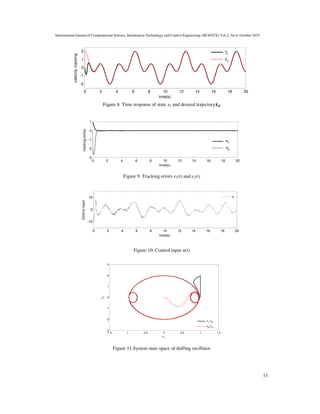
Figure 7. Time response of state x1 and desired trajectory xd.
-0.8 -0.6 -0.4 -0.2 0 0.2 0.4 0.6 0.8
0
0.1
0.2
0.3
0.4
0.5
0.6
0.7
0.8
0.9
1
µ
2
(s) µ
3
(s)µ
1
s)
0 2 4 6 8 10 12 14 16 18 20
-1
0
1
time(s)
Positiontracking
x1
yd

11. International Journal of Computational Science, Information Technology and Control Engineering (IJCSITCE) Vol.2, No.4, October 2015
11
Figure 8. Time response of state x2 and desired trajectory࢞ሶࢊ
Figure 9. Tracking errors e1(t) and e2(t)
Figure 10. Control input u(t)
Figure 11.System state space of duffing oscillator
0 2 4 6 8 10 12 14 16 18 20
-2
-1
0
1
2
time(s)
velocitytracking
x
2
y'
d
0 2 4 6 8 10 12 14 16 18 20
-3
-2
-1
0
1
time(s)
trackingerrors
e1
e2
0 2 4 6 8 10 12 14 16 18 20
-10
0
10
time(s)
Controlinput
u
-1.5 -1 -0.5 0 0.5 1 1.5
-3
-2
-1
0
1
2
3
x1
x2
x1
,x2
yd
,y'd

12. International Journal of Computational Science, Information Technology and Control Engineering (IJCSITCE) Vol.2, No.4, October 2015
12
Figure 12.Phase-plane trajectory of tracking errors(e1,e2)
Figure 13. Trajectories of sliding manifold s and its derivative ‫ݏ‬ሶ
According to the above simulation results, it is obvious that the tracking errors converge to zero
in a finite time, which implies that the proposed controller forces the system states to reach
quickly their references. Obviously, the phase trajectory of (e1, e2) converges directly to the phase
origin. In the same time, the implementation of Super Twisting algorithm in higher order sliding
mode control allows obtaining a smooth control signal (Figure10).
5. CONCLUSION
In this paper, the problem of stabilization orbit of uncertain chaotic system working in the
presence of uncertainties, external and internal disturbances is solved by incorporation of adaptive
interval type-2 control scheme and second order sliding mode approach using super-twisting
algorithm. The adaptive interval type-2 fuzzy systemsare introduced to approximate the unknown
part of system and Super Twisting gains. Based on the Laypunov stability criterion, the
adaptation law of adjustable parameters of the type-2 fuzzy system and the stability of closed loop
system are ensured. A simulation example has been presented to illustrate the robustnessand the
effectiveness of the proposed approach.
REFERENCES
[1] E. Tlelo-Cuautle,(2011) “Chaotic Systems”, JanezaTrdine 9, 51000 Rijeka, Croatia.
[2] I. Zelinka, S. Celikovsky, H. Richter & G. Chen, (2010) “Evolutionary Algorithms and Chaotic
Systems”, Studies in Computational Intelligence, vol. 267, Springer-Verlag Berlin Heidelberg.
[3] R. Femat, G. Solis-Perales, (2008), “Robust Synchronization of Chaotic Systems via Feedback”,
Springer-Verlag, Berlin Heidelberg.
-0.2 0 0.2 0.4 0.6 0.8 1 1.2
-15
-10
-5
0
5
e1
e2
practical trajectory
ideal sliding mode
0 2 4 6 8 10 12 14 16 18 20
-30
-20
-10
0
10
time(s)
sandsdot
Sliding surface
Derivative of sliding surface

13. International Journal of Computational Science, Information Technology and Control Engineering (IJCSITCE) Vol.2, No.4, October 2015
13
[4] K. Merat, J. A. Chekan, H. Salarieh, A. Alasty,(2014) “Linear optimal control of continuous time
chaotic systems”, ISA Transactions, vol. 53, pp. 1209-1215.
[5] L-X. Yang, Y-D. Chu, J.G. Zhang, X-F. Li & Y-X. Chang,(2009) “Chaos synchronization in
autonomous chaotic system via hybrid feedback control”, Chaos, Solitons and Fractals, vol. 41, pp.
214–223.
[6] J. H. Park,(2005) “Chaos synchronization of a chaotic system via nonlinear control”, Chaos,Solitons
and Fractals, Vol. 25, pp. 579–584.
[7] Q. Zhang & J-a. Lu,(2008) “Chaos synchronization of a new chaotic system via nonlinear control”,
Chaos, Solitons and Fractals, vol. 37, pp. 175– 179.
[8] Y. Jian, S. Bao, (2014) “Control and Synchronization of Fractional Unified Chaotic Systems via
Active Control Technique”, Proceedings of the 33rd Chinese Control Conference, pp.1977-1982.
[9] U. E. Vincent, (2008) “Chaos synchronization using active control and backstepping control: a
comparative analysis”, Nonlinear Analysis, Modelling and Control, Vol. 13, No. 2, pp. 253–261.
[10] B. A. Idowu, U. E. Vincent & A. N. Njah, (2008) “Control and synchronization of chaos in nonlinear
gyros via backstepping design”, International Journal of Nonlinear Science, Vol. 5, No.1 , pp. 11-19.
[11] F. Farivar, M.A. Shoorehdeli, (2012) “Fault tolerant synchronization of chaotic heavy symmetric
gyroscope systems versus external disturbances via Lyapunov rule-based fuzzy control”, ISA
Transactions, vol. 51, pp. 50-64.
[12] L-D. Zhao, J-B. Hu, J-A. Fang, W-X. Cui, Y-L. Xu, X. Wang, (2013) “Adaptive synchronization and
parameter identification of chaotic system with unknown parameters and mixed delays based on a
special matrix structure”, ISA Transactions, vol. 52, pp. 738-743.
[13] T-C Lin, C-H Kuo, (2011) “H-infinity synchronization of uncertain fractional order chaotic
systems:Adaptive fuzzy approach”, ISA Transactions, vol. 50, pp. 548-556.
[14] R. Hendel, F.Khaber, N. Essounbouli, (2015) “Chaos Control via Adaptive Interval Type-2 Fuzzy
Nonsingular Terminal Sliding Mode Control”, International Journal of Computational Science,
Information Technology and Control Engineering (IJCSITCE), Vol.2, pp. 19-31.
[15] N. Vasegh& A. K. Sedigh, (2009) “Chaos control in delayed chaotic systems via sliding mode based
delayed feedback”, Chaos, Solitons and Fractals, vol. 40, pp. 159–165.
[16] S. Vaidyanathan& S. Sampath, (2012) “Hybrid synchronization of hyperchaotic Chen systems via
sliding mode control”, Second International Conference, CCSIT Proceedings, Part II, India, pp. 257-
266.
[17] C. Yin, S. Dadras, S-m. Zhong& Y. Q. Chen, (2013) “Control of a novel class of fractional-order
chaotic systems via adaptive sliding mode control approach”, Applied Mathematical Modelling, vol.
37, pp. 2469–2483.
[18] X. Zhang, X. Liu & Q. Zhu, (2014) “Adaptive chatter free sliding mode control for a class of
uncertain chaotic systems”, Applied Mathematics and Computation, vol. 232, pp. 431 –435.
[19] M. Fazlyab, M.Z. Pedram, H. Salarieh, A. Alastyn, (2013) “Parameter estimation and interval type-2
fuzzy sliding mode control of a z-axis MEMS gyroscope”, ISA Transactions, vol.52, pp. 900-911.
[20] R. Hendel, F. Khaber, (2013) “Stabilizing Periodic Orbits of Chaotic System Using Adaptive Type-2
Fuzzy Sliding Mode Control”, Proceedings of The first International Conference on Nanoelectronics,
Communications and Renewable Energy ICNCRE’13 , Jijel, Algeria, p. 488-493.
[21] W. Perruquetti, J.P. Barbot, (2002) “Sliding mode control in engineering”, Marcel Dekker.
[22] X. Liu, Y. Han, (2014) “Finite time control for MIMO nonlinear system based on higher-order sliding
mode”, ISA Transactions, vol. 53, pp. 1838-1846.
[23] J. Wang, Q.Zong, R. Su, B.Tian, (2014) “Continuous high order sliding mode controller design for a
flexible air-breathing hypersonic vehicle”, ISA Transactions, vol. 53, pp. 690-698.
[24] A. Levant, (2007) “Principles of 2-sliding mode design”, Automatica, vol. 43, pp. 1247-1263.
[25] M. Benbouzid, B. Beltran, Y. Amirat, G. Yao, J. Han, H. Mangel, (2014) “Second-order sliding mode
control for DFIG-based wind turbines fault ride-through capability enhancement”, ISA Transactions,
vol. 53, pp. 827-833.
[26] A. Levant, (2001) “Universal SISO sliding mode controllers with finite-time convergence”, IEEE
Transactionson Automatic Control, vol. 46, pp. 1447– 1451.
[27] N.N. Karnik, J.M. Mendel, Q. Liang, (1999) “Type-2 fuzzy logic systems”, IEEE Trans. Fuzzy Syst,
vol. 7, pp. 643-658.
[28] J.E. Slotine, W.P. Li, (1991) “Applied Nonlinear Control”, Prentice-Hall, Englewood Cliffs, NJ.

14. International Journal of Computational Science, Information Technology and Control Engineering (IJCSITCE) Vol.2, No.4, October 2015
14
Authors
Rim Hendel received here engineering and Master degrees in Automatic from Setif
University (Setif 1), Algeria, in 2009 and 2012 respectively. From November 2012, she is
Ph.D. student in the Engineering Faculty with the QUERE laboratory at the University
ofSetif 1. Here research interests are higher order sliding mode control, fuzzy type-1 and
type-2 systems, nonlinear systems
Faridkhaber received his D.E.A in 1990 and his Master in 1992 degrees in industrial
control, and his PhD in 2006 from Setif University (Setif 1), Algeria, in automatic control.
He is currently a Professor in the Engineering Faculty from the same university. His
research interests include multivariable adaptive control, LMI control and type-2 fuzzy
control of renewable energy systems
NajibEssounbouli received his Maitrise from the University of Sciences and Technology
of Marrakech (FSTG) in Morocco, his D.E.A. in 2000, his Ph.D. in 2004, and its
Habilitation from Reims University of Champagne- Ardenne, all in Electrical
Engineering. From September 2005 to 2010, he has been an Assistant Professor with IUT
of Troyes, Reims Champagne Ardenne University. He is a currently a Professor and Head
of the Mechanical Engineering Department of IUT at Troyes, Reims University. His current research
interests are in the areas of fuzzy logic control, robust adaptive control, renewable energy and control drive.