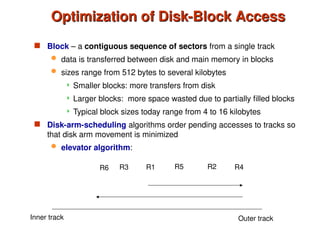
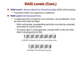
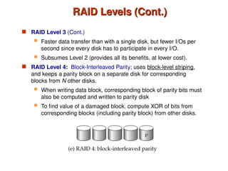
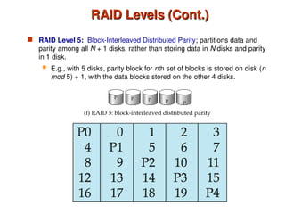
Storage and File Structure in DBMT ch10.ppt

Database System Concepts, 6th
Ed.
©Silberschatz, Korth and Sudarshan
See www.db-book.com for conditions on re-use
Chapter 10: Storage and File Structure

 Overview of Physical Storage Media
 Magnetic Disks
 RAID
 Tertiary Storage
 Storage Access
 File Organization
 Organization of Records in Files
 Data-Dictionary Storage

Classification of Physical Storage Media
Classification of Physical Storage Media
 Speed with which data can be accessed
 Cost per unit of data
 Reliability
 data loss on power failure or system crash
 physical failure of the storage device
 Can differentiate storage into:
 volatile storage: loses contents when power is switched off
 non-volatile storage:
 Contents persist even when power is switched off.
 Includes secondary and tertiary storage, as well as batter-
backed up main-memory.

Sequential vs. Random Access
Sequential vs. Random Access
 Random (Direct) access allows retrieval of any
data location in any order.
 E.g., RAM, HDD, SDD
 Sequential access requires visiting all previous
locations in sequential order to retrieve a given
location.
 E.g., Tapes

Physical Storage Media
Physical Storage Media
 Cache – fastest and most costly form of storage; volatile;
managed by the computer system hardware.
 Main memory:
 fast access (10s to 100s of nanoseconds; 1 nanosecond =
10–9
seconds)
 generally too small (or too expensive) to store the entire
database
 capacities of up to a few Gigabytes widely used currently
 Capacities have gone up and per-byte costs have
decreased steadily and rapidly (roughly factor of 2 every
2 to 3 years)
 Volatile — contents of main memory are usually lost if a
power failure or system crash occurs.

Physical Storage Media (Cont.)
 Flash memory - Widely used in embedded devices such as digital
cameras, phones, and USB keys
 Properties:
 Data survives power failure
 Data can be written at a location only once, but location can be
erased and written to again
 Can support only a limited number (10K – 1M) of write/erase
cycles.
 Erasing of memory has to be done to an entire bank of
memory
 Reads are roughly as fast as main memory
 But writes are slow (few microseconds), erase is slower
 Bandwidth (per chip): 40 MB/s (read), 20 MB/s (write)

 Magnetic-disk
 Data is stored on spinning disk, and read/written magnetically
 Primary medium for the long-term storage of data; typically stores
entire database.
 Data must be moved from disk to main memory for access, and
written back for storage
 Much slower access than main memory (more on this later)
 direct-access – possible to read data on disk in any order, unlike
magnetic tape
 Capacities range up to roughly 1.5 TB as of 2009
 Much larger capacity and cost/byte than main memory/flash
memory
 Growing constantly and rapidly with technology improvements
(factor of 2 to 3 every 2 years)
 Survives power failures and system crashes
 disk failure can destroy data, but is rare

 Optical storage
 non-volatile, data is read optically from a spinning disk
using a laser
 CD-ROM (640 MB) and DVD (4.7 to 17 GB) most
popular forms
 Blu-ray disks: 27 GB to 54 GB
 Write-one, read-many (WORM) optical disks used for
archival storage (CD-R, DVD-R, DVD+R)
 Multiple write versions also available (CD-RW, DVD-
RW, DVD+RW, and DVD-RAM)
 Reads and writes are slower than with magnetic disk
 Juke-box systems, with large numbers of removable
disks, a few drives, and a mechanism for automatic
loading/unloading of disks available for storing large
volumes of data

 Tape storage
 non-volatile, used primarily for backup (to recover from
disk failure), and for archival data
 sequential-access – much slower than disk
 very high capacity (40 to 300 GB tapes available)
 tape can be removed from drive  storage costs much
cheaper than disk, but drives are expensive
 Tape jukeboxes available for storing massive amounts
of data
 hundreds of terabytes (1 terabyte = 109
bytes) to
even multiple petabytes (1 petabyte = 1012
bytes)

Storage Hierarchy
Storage Hierarchy
“Tape is Dead. Disk is Tape. Flash is Disk. RAM Locality is King ."
Jim Gray (2006), Microsoft/IBM, Turing Award Winner 1998

Storage Hierarchy (Cont.)
Storage Hierarchy (Cont.)
 primary storage: Fastest media but volatile (cache, main
memory).
 secondary storage: next level in hierarchy, non-volatile,
moderately fast access time
 also called on-line storage
 E.g. flash memory, magnetic disks
 tertiary storage: lowest level in hierarchy, non-volatile, slow
access time
 also called off-line storage
 E.g. magnetic tape, optical storage

Magnetic Hard Disk Mechanism
Magnetic Hard Disk Mechanism
NOTE: Diagram is schematic, and simplifies the structure of actual disk drives

A Picture Is Worth Thousands of Words
A Picture Is Worth Thousands of Words
 https://www.youtube.com/watch?v=lBuXRRvuwXY

Magnetic Disks
Magnetic Disks
 Read-write head
 Positioned very close to the platter surface (almost touching it)
 Reads or writes magnetically encoded information.
 Surface of platter divided into circular tracks
 Over 50K-100K tracks per platter on typical hard disks
 Each track is divided into sectors.
 A sector is the smallest unit of data that can be read or written.
 Sector size typically 512 bytes
 Typical sectors per track: 500 to 1000 (on inner tracks) to 1000 to 2000 (on
outer tracks)
 To read/write a sector
 disk arm swings to position head on right track
 platter spins continually; data is read/written as sector passes under head
 Head-disk assemblies
 multiple disk platters on a single spindle (1 to 5 usually)
 one head per platter, mounted on a common arm.
 Cylinder i consists of ith
track of all the platters

Magnetic Disks (Cont.)
Magnetic Disks (Cont.)
 Disk controller – interfaces between the computer
system and the disk drive hardware.
 accepts high-level commands to read or write a sector
 initiates actions such as moving the disk arm to the
right track and actually reading or writing the data
 Computes and attaches checksums to each sector to
verify that data is read back correctly
 If data is corrupted, with very high probability stored
checksum won’t match recomputed checksum
 Ensures successful writing by reading back sector
after writing it
 Performs remapping of bad sectors

Disk Subsystem
Disk Subsystem
 Multiple disks connected to a computer system through a controller
 Controllers functionality (checksum, bad sector remapping) often
carried out by individual disks; reduces load on controller
 Disk interface standards families
 ATA (AT adaptor) range of standards
 SATA (Serial ATA)
 SCSI (Small Computer System Interconnect) range of standards
 SAS (Serial Attached SCSI)
 Several variants of each standard (different speeds and capabilities)

Disk Subsystem
 Disks usually connected directly to computer system
 In Storage Area Networks (SAN), a large number
of disks are connected by a high-speed network to a
number of servers
 In Network Attached Storage (NAS) networked
storage provides a file system interface using
networked file system protocol, instead of providing a
disk system interface

Performance Measures of Disks
Performance Measures of Disks
 Disk capacity is the size of the hard drive.
 = #cylinders * #tracks/cylinder * #sectors/track * #bytes/sector
 Access time – the time it takes from when a read or write request is
issued to when data transfer begins. Consists of:
 Seek time – time it takes to reposition the arm over the correct
track.
 Average seek time is 1/2 the worst case seek time.
– Would be 1/3 if all tracks had the same number of sectors,
and we ignore the time to start and stop arm movement
 4 to 10 milliseconds on typical disks
 Rotational latency – time it takes for the sector to be accessed to
appear under the head.
 Average latency is 1/2 of the worst case latency.
 4 to 11 milliseconds on typical disks (5400 to 15000 r.p.m.)
 Transfer time – time to transfer data to memory.

Performance Measures of Disks –
Performance Measures of Disks –
Cont’d
Cont’d
 Data-transfer rate – the rate at which data can be retrieved from or
stored to the disk.
 25 to 100 MB per second max rate, lower for inner tracks
 Multiple disks may share a controller, so rate that controller can
handle is also important
 E.g. SATA: 150 MB/sec, SATA-II 3Gb (300 MB/sec)
 Ultra 320 SCSI: 320 MB/s, SAS (3 to 6 Gb/sec)
 Fiber Channel (FC2Gb or 4Gb): 256 to 512 MB/s

Performance Measures (Cont.)
Performance Measures (Cont.)
 Mean time to failure (MTTF) – the average time the disk is
expected to run continuously without any failure.
 Typically 3 to 5 years
 Probability of failure of new disks is quite low,
corresponding to a
“theoretical MTTF” of 500,000 to 1,200,000 hours for a
new disk
 E.g., an MTTF of 1,200,000 hours for a new disk
means that given 1000 relatively new disks, on an
average one will fail every 1200 hours
 MTTF decreases as disk ages

Optimization of Disk-Block Access
Optimization of Disk-Block Access
 Block – a contiguous sequence of sectors from a single track
 data is transferred between disk and main memory in blocks
 sizes range from 512 bytes to several kilobytes
 Smaller blocks: more transfers from disk
 Larger blocks: more space wasted due to partially filled blocks
 Typical block sizes today range from 4 to 16 kilobytes
 Disk-arm-scheduling algorithms order pending accesses to tracks so
that disk arm movement is minimized
 elevator algorithm:
R1 R5 R2 R4
R3
R6
Inner track Outer track

Disk Scheduling
Disk Scheduling
Elevator Algorithm (SCAN)
https://www.youtube.com/watch?v=7G4I3cfjcoM
Multiple Disk Scheduling Algorithms
https://www.youtube.com/watch?v=6mVIK67xGrA7

Optimization of Disk Block Access (Cont.)
 Buffering – blocks read from disk are temporarily stored in a
memory buffer to satisfy future requests.
 Requires good eviction policies.
 Read-ahead – read consecutive blocks from the same track in the
in-memory buffer.
 Good for sequential access
 Bad for random access.

 File organization – optimize block access time by organizing the
blocks to correspond to how data will be accessed
 E.g. Store related information on the same or nearby cylinders.
 Files may get fragmented over time
 E.g. if data is inserted to/deleted from the file
 Or free blocks on disk are scattered, and newly created file
has its blocks scattered over the disk
 Sequential access to a fragmented file results in increased
disk arm movement
 Some systems have utilities to defragment the file system, in
order to speed up file access

 Nonvolatile write buffers speed up disk writes by writing blocks to a non-volatile
RAM buffer immediately
 Non-volatile RAM: battery backed up RAM or flash memory
 Even if power fails, the data is safe and will be written to disk when power
returns
 Controller then writes to disk whenever the disk has no other requests or
request has been pending for some time
 Database operations that require data to be safely stored before continuing can
continue without waiting for data to be written to disk
 Writes can be reordered to minimize disk arm movement
 Log disk – a disk devoted to writing a sequential log of block updates
 Used exactly like nonvolatile RAM
 Write to log disk is very fast since no seeks are required
 No need for special hardware (Nonvolatile-RAM)
 File systems typically reorder writes to disk to improve performance
 Journaling file systems write data in safe order to NV-RAM or log disk
 Reordering without journaling: risk of corruption of file system data
Optimization of Disk Block Access - Updates
Optimization of Disk Block Access - Updates

Flash Storage
 Widely used in embedded devices such as digital cameras,
phones, and USB keys
 NOR flash vs NAND flash
 NAND flash
 used widely for storage, since it is much cheaper than NOR flash
 requires page-at-a-time read (page: 512 bytes to 4 KB)
 erase is very slow (1 to 2 millisecs)
 erase block contains multiple pages
 can support only a limited number (10K – 1M) of write/erase cycles.
 bandwidth (per chip): 40 MB/s (read), 20 MB/s (write)

Solid State Drives
Solid State Drives
 NAND flash memory-based drives
 High voltage is able to change the configuration of a floating-gate
transistor
 State of the transistor interpreted as binary data
 Use multiple flash storage devices to provide higher transfer rates
28
Flash
memory chip
Data is striped
across all chips

Advantages of SSDs
Advantages of SSDs
 More resilient against physical damage
 No sensitive read head or moving parts
 Immune to changes in temperature
 Greatly reduced power consumption
 No mechanical, moving parts
 Much faster than hard drives
 >500 MB/s vs ~200 MB/s for hard drives
 No penalty for random access
 Each flash cell can be addressed directly
 No need to rotate or seek
 Extremely high throughput
 Although each flash chip is slow, they are RAIDed
29

RAID
RAID
 RAID: Redundant Arrays of Independent Disks
 disk organization techniques that manage a large numbers of disks,
providing a view of a single disk of
 high capacity and high speed by using multiple disks in parallel,
 high reliability by storing data redundantly, so that data can be recovered
even if a disk fails
 The chance that some disk out of a set of N disks will fail is much higher than
the chance that a specific single disk will fail.
 E.g., a system with 100 disks, each with MTTF of 100,000 hours (approx.
11 years), will have a system MTTF of 1000 hours (approx. 41 days)
 Techniques for using redundancy to avoid data loss are critical with large
numbers of disks
 Originally a cost-effective alternative to large, expensive disks
 I in RAID originally stood for ``inexpensive’’
 Today RAIDs are used for their higher reliability and bandwidth.
 The “I” is interpreted as independent

Improvement of Reliability via Redundancy
Improvement of Reliability via Redundancy
 Redundancy – store extra information that can be used to rebuild
information lost in a disk failure
 E.g., Mirroring (or shadowing)
 Duplicate every disk. Logical disk consists of two physical disks.
 Every write is carried out on both disks
 Reads can take place from either disk
 If one disk in a pair fails, data still available in the other
 Data loss would occur only if a disk fails, and its mirror disk also
fails before the system is repaired
– Probability of combined event is very small
» Except for dependent failure modes such as fire or
building collapse or electrical power surges
 Mean time to data loss depends on mean time to failure
and mean time to repair
 E.g. MTTF of 100,000 hours, mean time to repair of 10 hours gives
mean time to data loss of 500*106
hours (or 57,000 years) for a
mirrored pair of disks (ignoring dependent failure modes)

Improvement in Performance via Parallelism
Improvement in Performance via Parallelism
 Two main goals of parallelism in a disk system:
1. Load balance multiple small accesses to increase throughput
2. Parallelize large accesses to reduce response time.
 Improve transfer rate by striping data across multiple disks.
 Bit-level striping – split the bits of each byte across multiple disks
 In an array of eight disks, write bit i of each byte to disk i.
 Each access can read data at eight times the rate of a single disk.
 But seek/access time worse than for a single disk
 Bit level striping is not used much any more
 Block-level striping – with n disks, block i of a file goes to disk (i mod n) +
1
 Requests for different blocks can run in parallel if the blocks reside on
different disks
 A request for a long sequence of blocks can utilize all disks in parallel

RAID Levels
RAID Levels
 Schemes to provide redundancy at lower cost by using disk
striping combined with parity bits
 Different RAID organizations, or RAID levels, have differing
cost, performance and reliability characteristics
 RAID Level 1: Mirrored disks with block striping
 Offers best write performance.
 Popular for applications such as storing log files in a database system.
 RAID Level 0: Block striping; non-redundant.
 Used in high-performance applications where data loss is not critical.

RAID Levels (Cont.)
RAID Levels (Cont.)
 RAID Level 2: Memory-Style Error-Correcting-Codes (ECC) with bit striping.
 Theoretical model; very expensive to implement.
 RAID Level 3: Bit-Interleaved Parity
 a single parity bit is enough for error correction, not just detection, since
we know which disk has failed
 When writing data, corresponding parity bits must also be computed
and written to a parity bit disk
 To recover data in a damaged disk, compute XOR of bits from other
disks (including parity bit disk)

RAID Levels (Cont.)
RAID Levels (Cont.)
 RAID Level 3 (Cont.)
 Faster data transfer than with a single disk, but fewer I/Os per
second since every disk has to participate in every I/O.
 Subsumes Level 2 (provides all its benefits, at lower cost).
 RAID Level 4: Block-Interleaved Parity; uses block-level striping,
and keeps a parity block on a separate disk for corresponding
blocks from N other disks.
 When writing data block, corresponding block of parity bits must
also be computed and written to parity disk
 To find value of a damaged block, compute XOR of bits from
corresponding blocks (including parity block) from other disks.

RAID Levels (Cont.)
RAID Levels (Cont.)
 Provides higher I/O rates for independent block reads than Level 3
 block read goes to a single disk, so blocks stored on different
disks can be read in parallel
 Provides high transfer rates for reads of multiple blocks than no-
striping
 Before writing a block, parity data must be computed
 Can be done by using old parity block, old value of current block
and new value of current block (2 block reads + 2 block writes)
 Or by recomputing the parity value using the new values of
blocks corresponding to the parity block
– More efficient for writing large amounts of data sequentially
 Parity block becomes a bottleneck for independent block writes
since every block write also writes to parity disk

RAID Levels (Cont.)
RAID Levels (Cont.)
 RAID Level 5: Block-Interleaved Distributed Parity; partitions data and
parity among all N + 1 disks, rather than storing data in N disks and parity
in 1 disk.
 E.g., with 5 disks, parity block for nth set of blocks is stored on disk (n
mod 5) + 1, with the data blocks stored on the other 4 disks.

RAID Levels (Cont.)
RAID Levels (Cont.)
 Higher I/O rates than Level 4.
 Block writes occur in parallel if the blocks and their parity
blocks are on different disks.
 Subsumes Level 4: provides same benefits, but avoids bottleneck
of parity disk.
 RAID Level 6: P+Q Redundancy scheme; similar to Level 5, but
stores extra redundant information to guard against multiple disk
failures.
 Better reliability than Level 5 at a higher cost; not used as widely.

Choice of RAID Level
Choice of RAID Level
 Factors in choosing RAID level
 Monetary cost
 Performance: Number of I/O operations per second, and
bandwidth during normal operation
 Performance during failure
 Performance during rebuild of failed disk
 Including time taken to rebuild failed disk
 RAID 0 is used only when data safety is not important
 E.g. data can be recovered quickly from other sources
 Level 2 and 4 never used since they are subsumed by 3 and 5
 Level 3 is not used anymore since bit-striping forces single block
reads to access all disks, wasting disk arm movement, which
block striping (level 5) avoids
 Level 6 is growing in popularity.

RAID: A picture is worth a thousands words
RAID: A picture is worth a thousands words
 http://www.acnc.com/raidedu/1
 https://www.youtube.com/watch?v=aYSggTfz5LI

Optical Disks
Optical Disks
 Compact disk-read only memory (CD-ROM)
 Removable disks, 640 MB per disk
 Seek time about 100 msec (optical read head is heavier and slower)
 Higher latency (3000 RPM) and lower data-transfer rates (3-6 MB/s)
compared to magnetic disks
 Digital Video Disk (DVD)
 DVD-5 holds 4.7 GB , and DVD-9 holds 8.5 GB
 DVD-10 and DVD-18 are double sided formats with capacities of 9.4
GB and 17 GB
 Blu-ray DVD: 27 GB (54 GB for double sided disk)
 Slow seek time, for same reasons as CD-ROM
 Record once versions (CD-R and DVD-R) are popular
 data can only be written once, and cannot be erased.
 high capacity and long lifetime; used for archival storage
 Multi-write versions (CD-RW, DVD-RW, DVD+RW and DVD-RAM)
also available

Magnetic Tapes
Magnetic Tapes
 Hold large volumes of data and provide high transfer rates
 Few GB for DAT (Digital Audio Tape) format, 10-40 GB with DLT
(Digital Linear Tape) format, 100 GB+ with Ultrium format, and 330 GB
with Ampex helical scan format
 Transfer rates from few to 10s of MB/s
 Tapes are cheap, but cost of drives is very high
 Very slow access time in comparison to magnetic and optical disks
 limited to sequential access.
 Some formats (Accelis) provide faster seek (10s of seconds) at cost of
lower capacity
 Used mainly for backup, for storage of infrequently used information, and
as an off-line medium for transferring information from one system to
another.
 Tape jukeboxes used for very large capacity storage
 Multiple petabyes (1015
bytes)

10.47
Database System Concepts - 6th
Edition
File Organization, Record Organization
and Storage Access

File Organization
File Organization
 A database is stored as a collection of files.
 A file is a sequence of records.
 A record is a sequence of fields.
 One approach:
 assume record size is fixed
 each file has records of one particular type only
 different files are used for different relations
This case is easiest to implement; will consider variable length
records later.

Fixed-Length Records
Fixed-Length Records
 Simple approach:
 Store record i starting from byte n  (i – 1), where n is the size of
each record.
 Record access is simple but records may cross blocks
 Modification: do not allow records to cross block boundaries

Record Formats: Fixed Length
Record Formats: Fixed Length
 Information about field types same for all records in a file;
stored in system catalogs.
 Finding i’th field does not require scan of record.
Base address (B)
L1 L2 L3 L4
F1 F2 F3 F4
Address = B+L1+L2

Deletion of Fixed-Length Records
 Deletion of record i:
alternatives:
 move records i + 1, . . ., n to i, . . . , n – 1
 move record n to i
 do not move records, but link all free records on a
free list

Deleting record 3 and compacting
Deleting record 3 and compacting

Page Formats: Fixed Length Records
Page Formats: Fixed Length Records
 Record id = <page id, slot #>
 Moving records for free space management changes rid; may
not be acceptable.
Slot 1
Slot 2
Slot N
. . . Free
Space

alternatives:
Very expensive for files with large number of
records. Why?
 move record n to i
free list

Deleting record 3 and moving last record
Deleting record 3 and moving last record

alternatives:
Very expensive for files with large number of
records. Why?
 move record n to I
Alleviates some of the problems.
free list

Free Lists
Free Lists
 Store the address of the first deleted record in the file header.
 Use this first record to store the address of the second deleted record,
and so on
 Can think of these stored addresses as pointers since they “point” to
the location of a record.
 More space efficient representation: reuse space for normal attributes
of free records to store pointers. (No pointers stored in in-use records.)

Variable-Length Records
Variable-Length Records
 Variable-length records arise in database systems in several ways:
 Storage of multiple record types in a file.
 Record types that allow variable lengths for one or more fields such as
strings (varchar)
 Recall the question: What is the difference between char(100) and
varchar(100)?
 Record types that allow repeating fields (used in some older data
models).
 Attributes are stored in order
 Variable length attributes represented by fixed size (offset, length), with
actual data stored after all fixed length attributes
 Null values represented by null-value bitmap

Variable-Length Records: Slotted Page Structure
Variable-Length Records: Slotted Page Structure
 Slotted page header contains:
 number of record entries
 end of free space in the block
 location and size of each record
 Records can be moved around within a page to keep them contiguous
with no empty space between them.
 entry in the header must be updated.
 Pointers should not point directly to record — instead they should
point to the entry for the record in header.
Pointer to start
of free space.

Organization of Records in Files
Organization of Records in Files
 Heap – a record can be placed anywhere in the file where there
is space
 Sequential – store records in sequential order, based on the
value of the search key of each record
 Hashing – a hash function computed on some attribute of each
record
 The result specifies in which block of the file the record
should be placed
 Records of each relation may be stored in a separate file. In a
multitable clustering file organization records of several
different relations can be stored in the same file
 Motivation: store related records on the same block to
minimize I/O

Sequential File Organization
Sequential File Organization
 Suitable for applications that require sequential processing of
the entire file
 The records in the file are ordered by a search-key

Sequential File Organization (Cont.)
Sequential File Organization (Cont.)
 Deletion – use pointer chains
 Insertion –locate the position where the record is to be inserted
 if there is free space insert there
 if no free space, insert the record in an overflow block
 In either case, pointer chain must be updated
 Need to reorganize the file
from time to time to restore
sequential order

Multitable Clustering File Organization
Multitable Clustering File Organization
Store several relations in one file using a multitable clustering
file organization
department
instructor
multitable clustering
of department and
instructor

Multitable Clustering File Organization (cont.)
Multitable Clustering File Organization (cont.)
 Good for queries involving department instructor, and for queries
involving one single department and its instructors
 Bad for queries involving only department
 Results in variable size records
 Can add pointer chains to link records of a particular relation

Data Dictionary Storage
Data Dictionary Storage
 Information about relations
 names of relations
 names, types and lengths of attributes of each relation
 names and definitions of views
 integrity constraints
 User and accounting information, including passwords
 Statistical and descriptive data
 number of tuples in each relation
 Physical file organization information
 How relation is stored (sequential/hash/…)
 Physical location of relation
 Information about indices (Chapter 11)
The Data dictionary (also called system catalog) stores
metadata; that is, data about data, such as

Relational Representation of System Metadata
 Relational
representation on
disk
 Specialized data
structures
designed for
efficient access, in
memory

Storage Access
Storage Access
 A database file is partitioned into fixed-length storage units
called blocks. Blocks are units of both storage allocation
and data transfer.
 Database system seeks to minimize the number of
block transfers between the disk and memory.
 We can reduce the number of disk accesses by
keeping as many blocks as possible in main memory.
 Buffer – portion of main memory available to store copies
of disk blocks.
 Buffer manager – subsystem responsible for allocating
buffer space in main memory.

Buffer Manager in a DBMS
Buffer Manager in a DBMS
 Data must be in RAM for DBMS to operate
on it!
 Table of <frame#, pageid> pairs is
maintained.

Buffer Manager
Buffer Manager
 Programs call on the buffer manager when they need a block
from disk.
1. If the block is already in the buffer, buffer manager returns
the address of the block in main memory
2. If the block is not in the buffer, the buffer manager
1. Allocates space in the buffer for the block
1. Replacing (throwing out) some other block, if
required, to make space for the new block.
2. Replaced block written back to disk only if it was
modified since the most recent time that it was
written to/fetched from the disk.
2. Reads the block from the disk to the buffer, and returns
the address of the block in main memory to requester.

When a Page is Requested ...
When a Page is Requested ...
 If requested page is not in pool:
 Choose a frame for replacement
 If frame is dirty, write it to disk
 Read requested page into chosen frame
 Pin the page and return its address.
 If requests can be predicted (e.g., sequential scans)
pages can be pre-fetched several pages at a time!

Requesting a Page
Requesting a Page
22
MAIN MEMORY
DISK
disk page
free frames
BUFFER POOL
1 2 3 22 90
… …
Higher level DBMS
component
I need
page 3
Disk Mgr
Buf Mgr
I need
page 3
3 3

More on Buffer Management
More on Buffer Management
 Requestor of page must unpin it, and indicate
whether page has been modified:
 dirty bit is used for this.
 Page in pool may be requested many times,
 A pin count is used.
 To pin a page, pin_count++
 A page is a candidate for replacement iff pin
count = 0.

Releasing a Page
Releasing a Page
22
MAIN MEMORY
DISK
disk page
free frames
BUFFER POOL
1 2 3 22 90
… …
Higher level DBMS
component
I read page 3
and I’m done
with it
Disk Mgr
Buf Mgr
3

Releasing a Page
Releasing a Page
22
MAIN MEMORY
DISK
disk page
free frames
BUFFER POOL
1 2 3 22 90
… …
Higher level DBMS
component
I wrote on page
3 and I’m done
with it
Disk Mgr
Buf Mgr
3’
3’
3’

Buffer-Replacement Policies
Buffer-Replacement Policies
 Most operating systems replace the block least recently used
(LRU strategy)
 Idea behind LRU – use past pattern of block references as a
predictor of future references
 Queries have well-defined access patterns (such as sequential
scans), and a database system can use the information in a
user’s query to predict future references
 LRU can be a bad strategy for certain access patterns
involving repeated scans of data
 For example: when computing the join of 2 relations r and
s by a nested loops
for each tuple tr of r do
for each tuple ts of s do
if the tuples tr and ts match …
 Mixed strategy with hints on replacement strategy provided
by the query optimizer is preferable
Sequential
Flooding

2
1
1
4
LRU Sequential Flooding: Example
LRU Sequential Flooding: Example
MAIN MEMORY
BUFFER POOL
1 2 3 4
Higher level DBMS
component
I need
page 1
Disk Mgr
Buf Mgr
I need
page 2
3
I need
page 3
I need
page 4
DISK
I need
page 1
I need page
2…ARG!!!

Buffer-Replacement Policies (Cont.)
Buffer-Replacement Policies (Cont.)
 Pinned block – memory block that is not allowed to be
written back to disk.
 Toss-immediate strategy – frees the space occupied by a
block as soon as the final tuple of that block has been
processed
 Most recently used (MRU) strategy – system must pin the
block currently being processed. After the final tuple of that
block has been processed, the block is unpinned, and it
becomes the most recently used block.
 Buffer manager can use statistical information regarding the
probability that a request will reference a particular relation
 E.g., the data dictionary is frequently accessed.
Heuristic: keep data-dictionary blocks in main memory
buffer

Database System Concepts, 6th
Ed.
See www.db-book.com for conditions on re-use
End of Chapter 10
End of Chapter 10

Storage and File Structure in DBMT ch10.ppt

More Related Content

Similar to Storage and File Structure in DBMT ch10.ppt

More from priya523982

Recently uploaded

Storage and File Structure in DBMT ch10.ppt