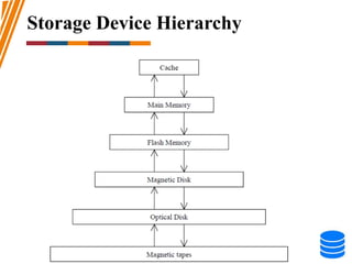
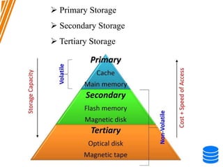
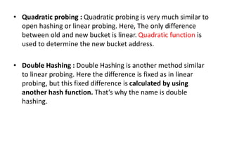
This document discusses various data storage concepts including physical storage media, file organization techniques, and indexing methods. It provides an overview of primary, secondary, and tertiary storage devices and their characteristics. It describes magnetic disks in detail including their structure, performance metrics, and optimization techniques. RAID levels 0-6 are explained along with their properties. Common file organization methods like sequential, heap, hash, and B+ tree are defined. Finally, basic indexing concepts and query processing operations are introduced.
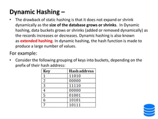
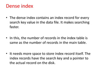
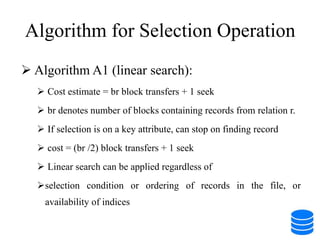
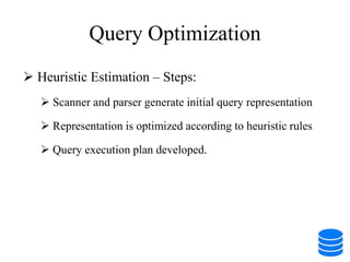
![Algorithm for Selection Operation
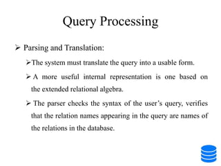
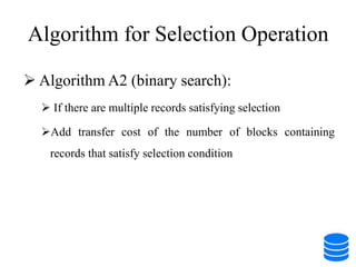
Algorithm A2 (binary search):
Applicable if selection is an equality comparison on the attribute
on which file is ordered.
Assume that the blocks of a relation are stored contiguously.
Cost estimate (number of disk blocks to be scanned):
cost of locating the first tuple by a binary search on the blocks
[log2(br)] * (tT + tS)](https://image.slidesharecdn.com/unitiii-230802072341-81eda92a/85/UNIT-III-pptx-100-320.jpg)
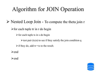
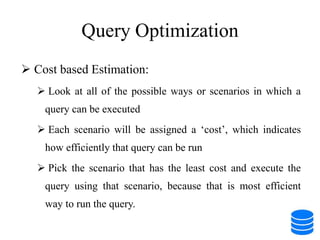
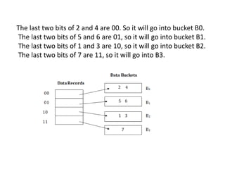
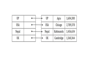
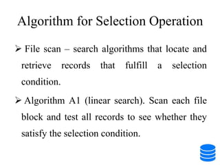
![Algorithm for JOIN Operation
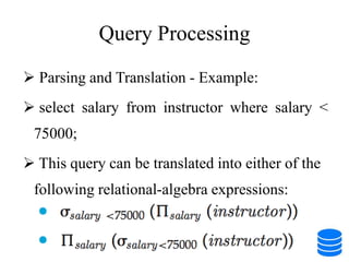
Merge Join
Sort both relations on their join attribute (if not already sorted
on the join attributes).
Merge the sorted relations to join them.
Can be used only for equijoins and natural joins
the cost of merge join is: br + bs block transfers + [br / bb]+ [bs
/ bb] seeks
+ the cost of sorting if relations are unsorted.](https://image.slidesharecdn.com/unitiii-230802072341-81eda92a/85/UNIT-III-pptx-107-320.jpg)
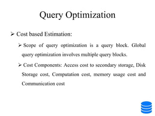
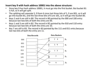
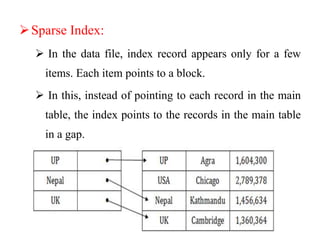
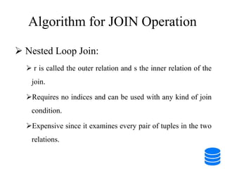
![Algorithm for JOIN Operation
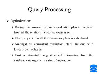
Hash Join:
The hash function is used h is used to partition tuples of
both the relations.
Cost: 3(br+bs)+4 x n block transfers + 2 ( [br/bb]+[bs/bb])
seeks.](https://image.slidesharecdn.com/unitiii-230802072341-81eda92a/85/UNIT-III-pptx-108-320.jpg)