Downloaded 15 times
![Answer to the Question No. 2
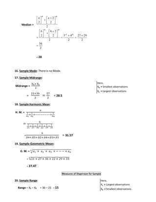
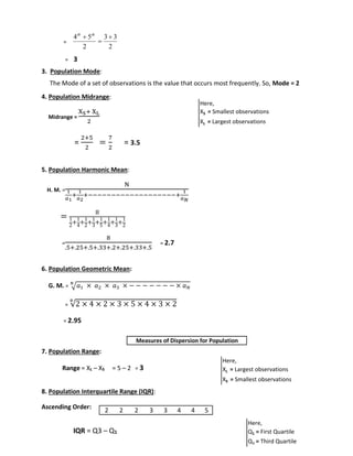
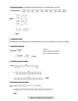
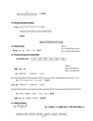
8. Population Interquartile Range (IQR):
Ascending Order:
21 22 22 22 22 23 27 28 29 33 36 36
IQR = Q3 – Q1
Q1 = .25(N+1)th = .25(12+1)th =3.25th
So, the first quartile is one quarter of the way from the 3rd observation (22) to the 4th (22).
Q1 = 22 + .25 (22 – 22) = 22+0 = 22
Again, Q3 = .75(N+1)th = .75(12+1)th = 9.75th
So, the third quartile is three quarters of the way from the 9th observation (29) to the 10th (33).
Q3 = 29 + .75(33 – 29) = 29 + 3 = 32
IQR = Q3 – Q1 = 32 – 22 = 10
9. Population Variance:
σ2
x =
2
Xi
− (26.75)= 2
=
8941
= 29.52
10. Population Standard Deviation:
σx= √휎2 = √29.52 = 5.43
11. Population Mean Absolute Deviation (MAD):
MAD =
x
i x The calculation for MAD are set out in the table:
Here,
Q1 = First Quartile
Q3 = Third Quartile
1 2
x
N
i
N
σ²x = Variance, μx = Population Mean = 26.75 [from (1)], N = 12
(21)²+ (22)²+ (27)²+ (36)²+ (22)²+ (29)²+ (22)²+ (23)²+ (22)²+ (28)²+ (36)²+ (33)²
12
715.56
12
σ = standard deviation, σ² = 29.52 [from (9)]
N
N
i
1
( )
μ = Population Mean = 26.75 [from (1)], N = 12](https://image.slidesharecdn.com/statisticsassignment2-140903062349-phpapp02/85/Statistics-assignment-2-1-320.jpg)
![Answer to the Question No. 2
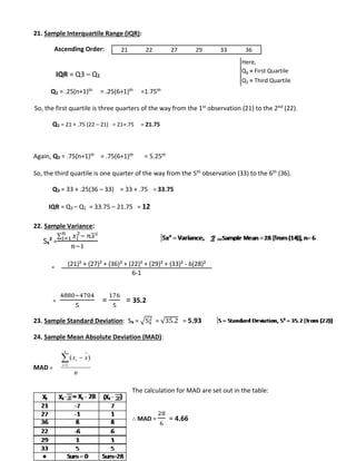
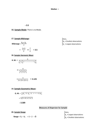
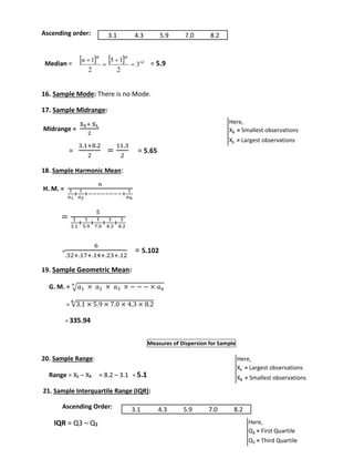
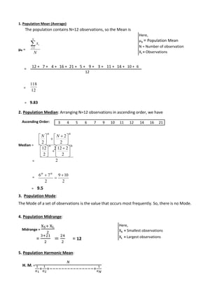
8. Population Interquartile Range (IQR):
Ascending Order:
21 22 22 22 22 23 27 28 29 33 36 36
IQR = Q3 – Q1
Q1 = .25(N+1)th = .25(12+1)th =3.25th
So, the first quartile is one quarter of the way from the 3rd observation (22) to the 4th (22).
Q1 = 22 + .25 (22 – 22) = 22+0 = 22
Again, Q3 = .75(N+1)th = .75(12+1)th = 9.75th
So, the third quartile is three quarters of the way from the 9th observation (29) to the 10th (33).
Q3 = 29 + .75(33 – 29) = 29 + 3 = 32
IQR = Q3 – Q1 = 32 – 22 = 10
9. Population Variance:
σ2
x =
2
Xi
− (26.75)= 2
=
8941
= 29.52
10. Population Standard Deviation:
σx= √휎2 = √29.52 = 5.43
11. Population Mean Absolute Deviation (MAD):
MAD =
x
i x The calculation for MAD are set out in the table:
Here,
Q1 = First Quartile
Q3 = Third Quartile
1 2
x
N
i
N
σ²x = Variance, μx = Population Mean = 26.75 [from (1)], N = 12
(21)²+ (22)²+ (27)²+ (36)²+ (22)²+ (29)²+ (22)²+ (23)²+ (22)²+ (28)²+ (36)²+ (33)²
12
715.56
12
σ = standard deviation, σ² = 29.52 [from (9)]
N
N
i
1
( )
μ = Population Mean = 26.75 [from (1)], N = 12](https://image.slidesharecdn.com/statisticsassignment2-140903062349-phpapp02/75/Statistics-assignment-2-1-2048.jpg)
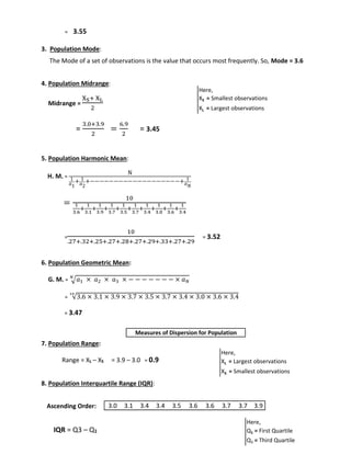
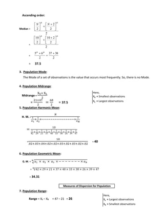
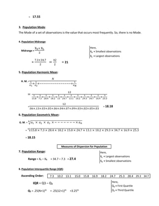
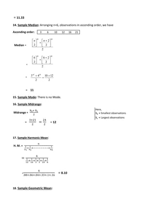
![∴ MAD =
57
12
= 4.75
Xi Xi - μx = Xi – 26.75 (Xi - μx)
21 -5.75 5.75
22 -4.75 4.75
27 0.25 0.25
36 9.25 9.25
22 -4.75 4.75
29 2.25 2.25
22 -4.75 4.75
23 -3.75 3.75
22 -4.75 4.75
28 1.25 1.25
36 9.25 9.25
33 6.25 6.25
* Sums = 0 Sums = 57
12. Population Coefficient of Variation:
C. V. =
σx
μx
× 100 =
5.43
26.75
× 100 = 20.29%
Measures of Central Tendency for Population
13. Population Midhinge:
Midhinge =
푄1+ 푄3
2
=
22 + 32
2
= 27
Measures of Central Tendency for Sample
Sample:
14. Sample Mean: The sample contains n=6, observations, so the Mean is
퐗̅
=
=
X
i 1
n
n
i
21 + 27 + 36 + 22 + 29 + 33
6
=
168
6
= 28
15. Sample Median: Arranging n=6, observations in ascending order, we have
Ascending order:
21 22 27 29 33 36
Q₁ = 22, Q₃ = 32 [from (8)]
21 27 36 22 29 33
C.V = coefficient of variation
σx = 5.43 [from (10)]
μx = 26.75 [from (1)]](https://image.slidesharecdn.com/statisticsassignment2-140903062349-phpapp02/85/Statistics-assignment-2-2-320.jpg)
![25. Sample Coefficient of Variation:
C. V. =
푆푥
푋
× 100 =
5.93
28
× 100 = 21.17%
Measures of Central Tendency for Sample
26. Sample Midhinge: Midhinge =
푄1+ 푄3
2
=
21.75 + 33.75
2
= 27.75
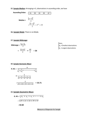
Answer to the Question No. 3
Population:
3.6 3.1 3.9 3.7 3.5 3.7 3.4 3.0 3.6 3.4
Measures of Central Tendency for Population
1. Population Mean (Average): The population contains N=10 observations, so the Mean is
μx =
=
=
x
i 1
N
9. 34
= 3.49
2. Population Median: Arranging N=10 observations in ascending order, we have
Ascending order:
Median =
=
=
Q₁ = 21.5, Q₃ = 33.75 [from (21)]
N
i
10
2
2
2
2
th th
N N
10 2
2
2
10
2
th th
5 6
3.5 3.6
2
2
th th
Here,
μx = Population Mean
N = Number of observation
Xi = Observations
3.6 + 3.1 + 3.9 + 3.7 + 3.5 + 3.7 + 3.4 + 3.0 + 3.6 + 3.4
10
3.0 3.1 3.4 3.4 3.5 3.6 3.6 3.7 3.7 3.9](https://image.slidesharecdn.com/statisticsassignment2-140903062349-phpapp02/85/Statistics-assignment-2-5-320.jpg)
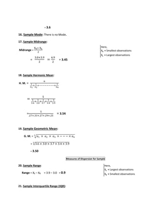
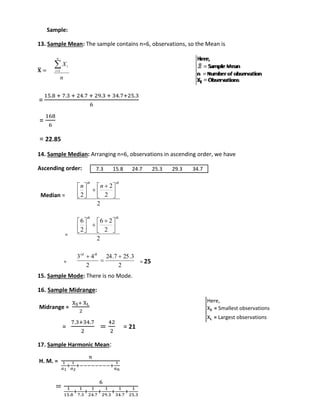
![Q1 = .25(N+1)th = .25(10+1)th =2.75th
So, the first quartile is three quarters of the way from the 2nd observation (3.1) to the 3rd (3.4).
Q1 = 3.1 + .75 (3.4 – 3.1) = 3.1+.225 = 3.325
Again, Q3 = .75(N+1)th = .75(10+1)th = 8.25th
So, the third quartile is one quarter of the way from the 8th observation (3.7) to the 9th (3.7).
Q3 = 3.7 + .25(3.7 – 3.7) = 3.7 + 0 = 3.7
IQR = Q3 – Q1 = 3.7 – 3.325 = .375
9. Population Variance:
σ2
x =
2
Xi
σx² = variance, μx = Population Mean = 3.49 [from (1)], N=10
(3.6)² + (3.1)² + (3.9)² + (3.7)² + (3.5)² + (3.7)² + (3.4)²+ (3.0)² + (3.6)² + (3.4)²
− = (3.49)2
=
122.49
= .069
10. Population Standard Deviation:
σx= √σ2 = √. 069 = .262
11. Population Mean Absolute Deviation (MAD):
MAD =
The calculation for MAD are set out in the table:
∴ MAD =
2.12
10
= .212
1 2
x
N
i
N
12.18
10
x
i x N
N
i
1
( )
10
σ = standard deviation, σ² = .069 [from (9)]
μ = Population Mean = 3.49 [from (1), N=10
Xi Xi - μx = Xi - 3.49 (Xi - μx)
3.6 0.11 0.11
3.1 -0.39 0.39
3.9 0.41 0.41
3.7 0.21 0.21
3.5 0.01 0.01
3.7 0.21 0.21
3.4 -0.09 0.09
3.0 -0.49 0.49
3.6 0.11 0.11
3.4 -0.09 0.09
* Sums = 0 Sums=2.12](https://image.slidesharecdn.com/statisticsassignment2-140903062349-phpapp02/85/Statistics-assignment-2-7-320.jpg)
![12. Population Coefficient of Variation:
C. V. =
σx
μx
× 100 =
.262
3.49
× 100 = 7.50%
Measures of Central Tendency for Population
13. Population Midhinge:
Midhinge =
푄1+ 푄3
2
=
3.325 + 3.7
2
= 3.51
Measures of Central Tendency for Sample
Sample:
14. Sample Mean: The sample contains n=6, observations, so the Mean is
퐗̅
=
=
X
i 1
n
3.6 + 3.0 + 3.7 + 3.4 + 3.9
5
=
17.6
5
= 3.52
15. Sample Median: Arranging n=6, observations in ascending order, we have
Ascending order:
Median =
n
i
1
th
rd
th n
3
5 1
2
2
Q₁ = 3.325, Q₃ = 3.7 [from (8)]
3.6 3.0 3.7 3.4 3.9
3.0 3.4 3.6 3.7 3.9
C.V = coefficient of variation
σx = .262 [from (10)]
μx = 3.49 [from (1)]](https://image.slidesharecdn.com/statisticsassignment2-140903062349-phpapp02/85/Statistics-assignment-2-8-320.jpg)
![Ascending Order:
IQR = Q3 – Q1
Q1 = .25(n+1)th = .25(5+1)th =1.5th
So, the first quartile is half quarter of the way from the 1st observation (3.0) to the 2nd (3.4).
Q1 = 3.0 + .5 (3.4 – 3.0) = 3.0+.215 = 3.215
Again, Q3 = .75(n+1)th = .75(5+1)th = 4.5th
So, the third quartile is half quarter of the way from the 4th observation (3.7) to the 5th (3.5).
Q3 = 3.7 + .5(3.9 – 3.7) = 3.7 + .1 = 3.8
IQR = Q3 – Q1 = 3.8 – 3.215 = 0.585
22. Sample Variance:
2 =
Sx
2− 푛푥² 푛푖
=1
Σ 푥푖
푛−1
=
=
62.42−61.95
4 =
.468
4
= .117
2 = √. 117 = 0.34
23. Sample Standard Deviation: Sx = √Sx
24. Sample Mean Absolute Deviation (MAD):
MAD =
i
x x
The calculation for MAD are set out in the table:
∴ MAD =
1.28
5
= .256
Here,
Q1 = First Quartile
Q3 = Third Quartile
n
n
i
1
( )
3.0 3.4 3.6 3.7 3.9
(3.6)² + (3.0)² + (3.7)² + (3.4)²+ (3.9)² - 5(3.52)²
5 - 1
Sx = standard deviation, Sx² = .117 [from (22)]](https://image.slidesharecdn.com/statisticsassignment2-140903062349-phpapp02/85/Statistics-assignment-2-10-320.jpg)
![25. Sample Coefficient of Variation:
C. V. =
푆푥
푋
× 100 =
0.34
3.52
× 100 = 9.65%
Measures of Central Tendency for Sample
26. Sample Midhinge: Midhinge =
푄1+ 푄3
2
=
3.215 + 3.8
2
= 3.50
Answer to the Question No – 4
Population:
Measures of Central Tendency for Population
1. Population Mean (Average): The population contains N=10 observations, so the Mean is
μx =
=
=
x
i 1
N
25
= 3.125
2. Population Median: Arranging N=8 observations in ascending order, we have
Ascending order:
Median =
=
σ₁ = 3.215, σ₃ = 3.8 [from (21)]
Here,
Q1 = First Quartile
Q3 = Third Quartile
2 4 2 3 5 4 3 2
N
i
8
2
2
2
2
th th
N N
8 2
2
2
8
2
th th
Here,
μx = Population Mean
N = Number of observation
Xi = Observations
2 + 4 + 2 + 3 + 5 + 4 + 3 + 2
8
2 2 2 3 3 4 4 5](https://image.slidesharecdn.com/statisticsassignment2-140903062349-phpapp02/85/Statistics-assignment-2-11-320.jpg)
![Q1 = .25(N+1)th = .25(8+1)th =2.25th
So, the first quartile is one quarter of the way from the 2nd observation (2) to the 3rd (2).
Q1 = 2 + .25 (2 – 2) = 2 + 0 = 2
Again, Q3 = .75(N+1)th = .75(8+1)th = 6.75th
So, the third quartile is three quarters of the way from the 6th observation (4) to the 7th (4).
Q3 = 4 + .75(4 – 4) = 4 + 0 = 4
IQR = Q3 – Q1 = 4 – 2 = 2
9. Population Variance:
σ2
x =
2
Xi
− (3.12 = 5 ) 2
=
87
= 1.11
10. Population Standard Deviation:
σx= √σ2 = √1.11 = 1.05
11. Population Mean Absolute Deviation (MAD):
MAD =
The calculation for MAD are set out in the table:
1 2
x
N
i
N
9.765
8
x
i x N
N
i
1
( )
σx² = variance, μx = Population Mean = 3.125 [from (1)], N=8
(2)²+ (4)²+ (2)²+ (3)²+ (5)²+ (4)²+ (3)²+ (2)²
8
σ = standard deviation, σ² = 3.125 [from (9)]
μ = Population Mean = 3.125 [from (1), N=8
Xi Xi - μx = Xi - 3.125 (Xi - μx)
2 -1.125 1.125
4 0.875 0.875
2 -1.125 1.125
3 -0.125 0.125
5 1.875 1.875
4 0.875 0.875
3 -0.125 0.125
2 -1.125 1.125
* Sums = 0 Sums=7.25](https://image.slidesharecdn.com/statisticsassignment2-140903062349-phpapp02/85/Statistics-assignment-2-13-320.jpg)
![∴ MAD =
2.25
8
= .90625
12. Population Coefficient of Variation:
C. V. =
σx
μx
× 100 =
1.05
3.125
× 100 = 33.6%
Measures of Central Tendency for Population
13. Population Midhinge:
Midhinge =
푄1+ 푄3
2
=
2 + 4
2
= 3
Measures of Central Tendency for Sample
Sample:
14. Sample Mean: The sample contains n=4, observations, so the Mean is
X̅
=
=
X
i 1
n
n
i
2 + 4 + 3 + 5
4
=
14
4
= 3.5
15. Sample Median: Arranging n=4, observations in ascending order, we have
th th
n n
Ascending order:
C.V = coefficient of variation
σx = 1.05 [from (10)]
μx = 3.125 [from (1)]
Q₁ = 2, Q₃ = 4 [from (8)]
2 4 3 5
2 3 4 5
3 4
2
2 3
2
2
4 2
2
4
2
2
2
2
2
nd rd
th th](https://image.slidesharecdn.com/statisticsassignment2-140903062349-phpapp02/85/Statistics-assignment-2-14-320.jpg)
![21. Sample Interquartile Range (IQR):
Ascending Order:
IQR = Q3 – Q1
Q1 = .25(n+1)th = .25(4+1)th =1.25th
So, the first quartile is three quarters of the way from the 1st observation (2) to the 2nd (3).
Q1 = 2 + .25(3 – 2) = 2 + .25 = 2.25
Again, Q3 = .75(n+1)th = .75(4+1)th = 3.75th
So, the third quartile is threequarters of the way from the 3rd observation (4) to the 4th (5).
Q3 = 4+ .75(5 – 4) = 4 + .75 = 4.75
IQR = Q3 – Q1 = 4.75 – 3.75 = 1
22. Sample Variance:
2 =
Sx
2− 푛푥² 푛푖
=1
Σ 푥푖
푛−1
=
=
54−49
3 =
5
3
= 1.6666
2 = √1.6666 = 1.29
23. Sample Standard Deviation: Sx = √Sx
24. Sample Mean Absolute Deviation (MAD):
MAD =
i
x x
The calculation for MAD are set out in the table:
∴ MAD =
4
4
= 1
Here,
Q1 = First Quartile
Q3 = Third Quartile
n
n
i
1
( )
2 3 4 5
(2)²+ (4)²+ (3)²+ (5)² - 4(3.5)²
4 - 1
Sx = standard deviation, Sx² = 1.6666 [from (22)]](https://image.slidesharecdn.com/statisticsassignment2-140903062349-phpapp02/85/Statistics-assignment-2-16-320.jpg)
![25. Sample Coefficient of Variation:
C. V. =
푆푥
푋
× 100 =
1.29
3.5
× 100 = 36.85%
Measures of Central Tendency for Sample
26. Sample Midhinge: Midhinge =
푄1+ 푄3
2
=
2.25 + 4.75
2
= 3.5
Answer to the Question No. 5
Population:
42 29 21 37 40 33 38 26 39 47
Measures of Central Tendency for Population
1. Population Mean (Average):
The population contains N=10 observations, so the Mean is
μx =
=
=
x
i 1
N
N
i
42 + 29 + 21 + 37 + 40 + 33 + 38 + 26 + 39 + 47
352
10
= 35.2
Q₁ = 2.25, Q₃ = 4.75 [from (21)]
Here,
μx = Population Mean
N = Number of observation
Xi = Observations
10
2. Population Median: Arranging N=10 observations in ascending order, we have
21 26 29 33 37 38 39 40 42 47](https://image.slidesharecdn.com/statisticsassignment2-140903062349-phpapp02/85/Statistics-assignment-2-17-320.jpg)
![8. Population Interquartile Range (IQR):
Ascending Order:
IQR = Q3 – Q1
Q1 = .25(N+1)th = .25(10+1)th =2.75th
So, the first quartile is three quarters of the way from the 2nd observation (26) to the 3rd (29).
Q1 = 26 + .75 (29 – 26) = 26+2.25 = 28.25
Again, Q3 = .75(N+1)th = .75(10+1)th = 8.25th
So, the third quartile is one quarter of the way from the 8th observation (40) to the 9th (42).
Q3 = 40 + .25(42 – 40) = 40 + 0.5 = 40.5
IQR = Q3 – Q1 = 40.5 – 28.5
= 12
9. Population Variance:
σ2
x =
2
Xi
− = (35.2)2
=
12954
= 56.36
10. Population Standard Deviation:
σx= √휎2 = √56.36 = 7.50
11. Population Mean Absolute Deviation (MAD):
MAD =
x
i x The calculation for MAD are set out in the table:
Here,
Q1 = First Quartile
Q3 = Third Quartile
1 2
x
N
i
N
1239.04
10
N
N
i
1
( )
21 26 29 33 37 38 39 40 42 47
σx² = variance, μx = Population Mean = 35.2 [from (1)], N=10
(42)² + (29)² + (21)² + (37)² + (40)² + (33)² + (38)² + (26)² + (39)² + (47)²
10
σ = standard deviation, σ² = 56.36 [from (9)]
μ = Population Mean = 35.2 [from (1), N=10](https://image.slidesharecdn.com/statisticsassignment2-140903062349-phpapp02/85/Statistics-assignment-2-19-320.jpg)
![∴ MAD =
63.6
10
= 6.36
Xi Xi - μx = Xi - 35.2 (Xi - μx)
42 6.8 6.8
29 -6.2 6.2
21 -14.2 14.2
37 1.8 1.8
40 4.8 4.8
33 -2.2 2.2
38 2.8 2.8
26 -9.2 9.2
39 3.8 3.8
47 11.8 11.8
* Sums = 0 Sums=63.6
12. Population Coefficient of Variation:
C. V. =
σx
μx
× 100 =
7.50
35.2
× 100 = 21.30%
Measures of Central Tendency for Population
13. Population Midhinge:
Midhinge =
푄1+ 푄3
2
=
28.5+ 40.5
2
= 34.5
Measures of Central Tendency for Sample
Sample:
14. Sample Mean: The sample contains n=5, observations, so the Mean is
퐗̅
=
=
X
i
1
29 + 21 + 33 + 39 + 47
5
=
169
5
= 33.8
n
n
i
C.V = coefficient of variation
σx = 7.50 [from (10)]
μx = 35.2 [from (1)]
Q₁ = 28.5, Q₃ = 40.5 [from (21)]
29 21 33 39 47](https://image.slidesharecdn.com/statisticsassignment2-140903062349-phpapp02/85/Statistics-assignment-2-20-320.jpg)
![20. Sample Range:
Range = XL – XS = 47 – 21 = 26
21. Sample Interquartile Range (IQR):
Ascending Order:
IQR = Q3 – Q1
Q1 = .25(n+1)th = .25(5+1)th =1.5th
Here,
XL = Largest observations
XS = Smallest observations
Here,
Q1 = First Quartile
Q3 = Third Quartile
So, the first quartile is half quarter of the way from the 1st observation (21) to the 2nd (29).
Q1 = 21 + .5(29 – 21) = 21 + 4 = 25
Again, Q3 = .75(n+1)th = .75(5+1)th = 4.5th
So, the third quartile is half quarter of the way from the 4th observation (39) to the 5th (47).
Q3 = 39 + .5(47 – 39) = 39 + 4 = 43
IQR = Q3 – Q1 = 43 – 25 = 18
22. Sample Variance:
2 =
Sx
2− 푛푥² 푛푖
=1
Σ 푥푖
푛−1
=
=
6101−5712.2
4
=
388.8
4
= 97.2
2 = √97.2 = 9.85
23. Sample Standard Deviation: Sx = √푆푥
24. Sample Mean Absolute Deviation (MAD):
i
x x
MAD =
The calculation for MAD are set out in the table:
n
n
i
1
( )
21 29 33 39 47
(29)²+ (21)²+ (33)²+ (39)²+ (47)² - 5(33.8)²
5 - 1
Sx = standard deviation, Sx² = 97.2 [from (22)]](https://image.slidesharecdn.com/statisticsassignment2-140903062349-phpapp02/85/Statistics-assignment-2-22-320.jpg)
![∴ MAD =
36.8
5
= 7.36
25. Sample Coefficient of Variation:
C. V. =
푆푥
푋
× 100 =
9.85
33.8
× 100 = 29.14%
Measures of Central Tendency for Sample
26. Sample Midhinge: Midhinge =
푄1+ 푄3
2
=
25 + 43
2
= 34
Answer to the Question No. 6
Population:
10.2 3.1 5.9 7.0 3.7 2.9 6.8 7.3 8.2 4.3
Measures of Central Tendency for Population
1. Population Mean (Average):
The population contains N=10 observations, so the Mean is
μx =
=
=
x
i 1
N
59.4
= 5.94
Q₁ = 25, Q₃ = 43 [from (21)]
N
i
10
Here,
μx = Population Mean
N = Number of observation
Xi = Observations
10.2 + 3.1 + 5.9 + 7.0 + 3.7 + 2.9 + 6.8 + 7.3 + 8.2 + 4.3
10](https://image.slidesharecdn.com/statisticsassignment2-140903062349-phpapp02/85/Statistics-assignment-2-23-320.jpg)
![7. Population Range:
Range = XL – XS = 10.2 – 2.9 = 7.3
8. Population Interquartile Range (IQR):
Ascending Order:
IQR = Q3 – Q1
2.9 3.1 3.7 4.3 5.9 6.8 7.0 7.3 8.2 10.2
Q1 = .25(N+1)th = .25(10+1)th =2.75th
So, the first quartile is three quarters of the way from the 2nd observation (3.1) to the 3rd (3.7).
Q1 = 3.1 + .75(3.7 – 3.1) = 3.1+.45 = 3.55
Again, Q3 = .75(N+1)th = .75(10+1)th = 8.25th
So, the third quartile is one quarter of the way from the 8th observation (7.3) to the 9th (8.2).
Q3 = 7.3 + .25(8.2 – 7.3) = 7.3 + .225 = 7.525
IQR = Q3 – Q1 = 7.525 – 3.55 = 3.975
9. Population Variance:
σ2
x =
2
Xi
− (5.94)= 2
=
404.82
= 5.20
10. Population Standard Deviation: σx= √σ2 = √5.20 = 2.28
11. Population Mean Absolute Deviation (MAD):
MAD =
x
i x The calculation for MAD are set out in the table:
Here,
XL = Largest observations
XS = Smallest observations
Here,
Q1 = First Quartile
Q3 = Third Quartile
1 2
x
N
i
N
35.28
10
N
N
i
1
( )
σx² = variance, μx = Population Mean = 5.94 [from (1)], N=10
(10.2)² + (3.1)² + (5.9)² + (7.0)² + (3.7)² + (2.9)² + (6.8)²+ (7.3)² + (8.2)² + (4.3)²
10
σ = standard deviation, σ² = 5.20 [from (9)]
μ = Population Mean = 5.94 [from (1), N=10](https://image.slidesharecdn.com/statisticsassignment2-140903062349-phpapp02/85/Statistics-assignment-2-25-320.jpg)
![∴ MAD =
19.6
10
= 1.96
Xi Xi - μx = Xi - 5.94 (Xi - μx)
10.2 4.26 4.26
3.1 -2.84 2.84
5.9 -0.04 0.04
7.0 1.06 1.06
3.7 -2.24 2.24
2.9 -3.04 3.04
6.8 0.86 0.86
7.3 1.36 1.36
8.2 2.26 2.26
4.3 -1.64 1.64
* Sums = 0 Sums 19.6
12. Population Coefficient of Variation:
C. V. =
σx
μx
× 100 =
2.28
5.94
× 100 = 38.38%
C.V = coefficient of variation
σx = 2.28 [from (10)]
μx = 5.94 [from (1)]
Measures of Central Tendency for Population
13. Population Midhinge:
Midhinge =
푄1+ 푄3
2
=
3.55 + 7.525
2
= 5.5375
σ₁ = 3.215, σ₃ = 3.8 [from (8)]
Measures of Central Tendency for Sample
Sample:
3.1 5.9 7.0 4.3 8.2
14. Sample Mean: The sample contains n=5, observations, so the Mean is
퐗̅
=
=
X
i 1
n
n
i
3.1 + 5.9 + 7.0 + 4.3 + 8.2
5
28.5
5
= 5.7
=
Here,
Q1 = First Quartile
Q3 = Third Quartile
15. Sample Median: Arranging n=5, observations in ascending order, we have](https://image.slidesharecdn.com/statisticsassignment2-140903062349-phpapp02/85/Statistics-assignment-2-26-320.jpg)
![Q1 = .25(n+1)th = .25(5+1)th =1.5th
So, the first quartile is three quarters of the way from the 1st observation (3.1) to the 2nd (4.3).
Q1 = 3.1 + .75 (4.3 – 3.1) = 3.1 + .90 = 4
Again, Q3 = .75(n+1)th = .75(5+1)th = 4.5th
So, the third quartile is one quarter of the way from the 4th observation (7.0) to the 5th (8.2).
Q3 = 7.0 + .25(8.2 – 7.0) = 7.0 + .30 = 7.3
IQR = Q3 – Q1 = 7.3 – 4 = 3.3
22. Sample Variance:
Sx
Σ 푥푖
2 =
2− 푛푥² 푛푖
=1
푛−1
=
=
(3.1)²+ (4.3)²+ (5.9)²+ (7.0)²+ (8.2)² - 5(5.7)²
16.7
4
= 4.175
2 = √4.175 = 2.04
5 - 1
23. Sample Standard Deviation: Sx = √Sx
24. Sample Mean Absolute Deviation (MAD):
MAD =
i
x x
( )
n
n
i
1
The calculation for MAD are set out in the table:
∴ MAD =
8
5
= 1.6
25. Sample Coefficient of Variation:
Sx = standard deviation, Sx² = 4.175 [from (22)]](https://image.slidesharecdn.com/statisticsassignment2-140903062349-phpapp02/85/Statistics-assignment-2-28-320.jpg)
![C. V. =
Sx
X
× 100 =
2.04
5.7
× 100 = 35.75%
Measures of Central Tendency for Sample
26. Sample Midhinge: Midhinge =
푄1+ 푄3
2
=
4 + 7.3
2
= 5.65
Answer to the Question No. 7
Population:
15.8 7.3 28.4 18.2 15.0 24.7 13.1 10.2 29.3 34.7 16.9 25.3
Measures of Central Tendency for Population
1.Population Mean (Average):
The population contains N=12 observations, so the Mean is
μx =
=
=
x
i 1
N
238.9
= 19.90
2. Population Median: Arranging N=12 observations in ascending order, we have
Ascending Order:
Median =
=
=
Q₁ = 4, Q₃ = 7.3 [from (21)]
N
i
12
2
2
2
2
th th
N N
12 2
2
2
12
2
th th
6 7
16.9 18.2
2
2
th th
Here,
μx = Population Mean
N = Number of observation
Xi = Observations
15.8 + 7.3 + 28.4 + 18.2 + 15.0 + 24.7 + 13.1 + 10.2 + 29.3 + 34.7 + 16.9 + 25.3
12
7.3 10.2 13.1 15.0 15.8 16.9 18.2 24.7 25.3 28.4 29.3 34.7](https://image.slidesharecdn.com/statisticsassignment2-140903062349-phpapp02/85/Statistics-assignment-2-29-320.jpg)
![So, the first quartile is one quarter of the way from the 3rd observation (13.1) to the 4th (15.0).
Q1 = 13.1 + .25(15 – 13.1) = 13.1+.48 = 13.58
Again, Q3 = .75(N+1)th = .75(12+1)th = 9.75th
So, the third quartile is three quarters of the way from the 9th observation (25.3) to the 10th (28.4).
Q3 = 25.3 + .75(28.4 – 25.3) = 25.3 + 2.325 = 27.63
IQR = Q3 – Q1 = 27.625 – 13.5 = 14.13
9. Population Variance:
σ2
x =
2
Xi
σx² = variance, μx = Population Mean = 19.90 [from (1)], N=12
(15.8)² + (7.3)² + (28.4)² + (18.2)² + (15.0)² + (24.7)² + (13.1)²+ (10.2)² + (29.3)² + (34.7)² (16.9)² + (25.3)²
− (19.90)= 2
=
5539.75
= 65.63
10. Population Standard Deviation: σx= √σ2 = √65.63 = 8.10
11. Population Coefficient of Variation:
C. V. =
σx
μx
× 100 =
8.10
19.90
× 100 = 40.70%
Measures of Central Tendency for Population
12. Population Midhinge:
Midhinge =
푄1+ 푄3
2
=
13.58 + 27.63
2
= 20.61
Measures of Central Tendency for Sample
1 2
x
N
i
N
396.01
12
12
σ = standard deviation, σ² = 65.63 [from (9)]
C.V = coefficient of variation
σx = 8.10 [from (10)]
μx = 19.90 [from (1)]
σ₁ = 13.58, σ₃ = 27.63 [from (8)]
Here,
Q1 = First Quartile
Q3 = Third Quartile
15.8 7.3 24.7 29.3 34.7 25.3](https://image.slidesharecdn.com/statisticsassignment2-140903062349-phpapp02/85/Statistics-assignment-2-31-320.jpg)
![=
3615.69−3132.735
5
=
482.955
5
= 95.591
2 = √95.591 = 9.77
22. Sample Standard Deviation: Sx = √Sx
23. Sample Mean Absolute Deviation (MAD):
MAD =
i
x x
The calculation for MAD are set out in the table:
∴ MAD =
45.2
6
= 7.53
24. Sample Coefficient of Variation:
C. V. =
Sx
X
× 100 =
9.77
22.85
× 100 = 42.75%
Measures of Central Tendency for Sample
25. Sample Midhinge: Midhinge =
푄1+ 푄3
2
=
13.675 + 30.65
2
= 22.16
Answer to the Question No. 16
Population:
Measures of Central Tendency for Population
n
n
i
1
( )
Sx = standard deviation, Sx² = 95.591 [from (21)]
Q₁ = 13.675, Q₃ = 30.65 [from (20)]
12 7 4 16 21 5 9 3 11 14 10 6](https://image.slidesharecdn.com/statisticsassignment2-140903062349-phpapp02/85/Statistics-assignment-2-34-320.jpg)
![=
12
1
12
+
1
7
+
1
4
1
16
+
1
21
+
+
1
5
1
9
+
+
1
3
+
1
11
+
1
14
+
1
10
+
1
6
=
12
.08+.14+.25+.06+.04+.2+.11+.13+.09+.07+.1+.16
= 7.40
6. Population Geometric Mean:
퐍
G. M. = √푎1 × 푎2 × 푎3 × − − − − − − − × 푎푁
= √12 × 7 × 4 × 16 × 21 × 5 × 9 × 3 × 11 × 14 × 10 × 6 ퟏퟐ
= 6.95
7. Population Range:
Range = XL – XS = 21 – 3 = 18
8. Population Interquartile Range (IQR):
Ascending Order:
IQR = Q3 – Q1
Q1 = .25(N+1)th = .25(12+1)th =3.25th
So, the first quartile is one quarter of the way from the 3rd observation (5) to the 4th (6).
Q1 = 5 + .25(6 – 5) = 5 +.25 = 5.25
Again, Q3 = .75(N+1)th = .75(12+1)th = 9.75th
So, the third quartile is three quarters of the way from the 9th observation (12) to the 10th (14).
Q3 = 12 + .75(14 – 12) = 12 + 1.5 = 13.5
IQR = Q3 – Q1 = 13.5 – 5.25 = 8.25
9. Population Variance:
σ2
x =
Here,
XL = Largest observations
XS = Smallest observations
Here,
Q1 = First Quartile
Q3 = Third Quartile
2
Xi
1 2
x
N
i
N
Measures of Dispersion for Population
3 4 5 6 7 9 10 11 12 14 16 21
σx² = variance, μx = Population Mean = 9.83 [from (1)], N=12
(12)² + (7)² + (4)² + (16)² + (21)² + (5)² + (9)²+ (3)² + (11)² + (14)² + (10)² + (6)²
12](https://image.slidesharecdn.com/statisticsassignment2-140903062349-phpapp02/85/Statistics-assignment-2-36-320.jpg)
![= − (9.83)2
=
147 4
= 26.21
10. Population Standard Deviation: σx= √σ2 = √26.21 = 5.11
11. Population Coefficient of Variation:
C. V. =
σx
μx
× 100 =
5.11
9.83
× 100 = 51.98%
Measures of Central Tendency for Population
12. Population Midhinge:
Midhinge =
푄1+ 푄3
2
=
5.25 + 13.5
2
= 9.375
Measures of Central Tendency for Sample
Sample:
13. Sample Mean: The sample contains n=6, observations, so the Mean is
퐗̅
=
=
X
i 1
12 + 16 + 21 + 3 + 10+ 6
6
=
68
6
62. 96
12
n
n
i
σ = standard deviation, σ² = 26.21 [from (9)]
C.V = coefficient of variation
σx = 5.11 [from (10)]
μx = 9.83 [from (1)]
Q₁ = 5.25, Q₃ = 13.5 [from (8)]
12 16 21 3 10 6](https://image.slidesharecdn.com/statisticsassignment2-140903062349-phpapp02/85/Statistics-assignment-2-37-320.jpg)
![푛
G. M. = √푎1 × 푎2 × 푎3 × − − − × 푎푛
= √12 × 16 × 21 × 3 × 10 × 6 ퟔ
= 9.47
Measures of Dispersion for Sample
19. Sample Range:
Range = XL – XS = 21 – 3 = 18
20. Sample Interquartile Range (IQR):
Ascending Order:
IQR = Q3 – Q1
Q1 = .25(n+1)th = .25(6+1)th =1.75th
So, the first quartile is three quarters of the way from the 1st observation (3) to the 2nd (6).
Q1 = 3 + .75 (6 – 3) = 3 + 2.25 = 5.25
Again, Q3 = .75(n+1)th = .75(6+1)th = 5.25th
So, the third quartile is one quarter of the way from the 5th observation (16) to the 6th (21).
Q3 = 16 + .25(21 – 16) = 16 + 1.25 = 17.25
IQR = Q3 – Q1 = 17.25 – 5.25 = 12
21. Sample Variance:
2 =
Sx
2− 푛푥² 푛푖=1
Σ 푥푖
푛−1
=
=
986−770.21
5
=
215.79
5
= 43.15
2 = √43.15 = 6.56
22. Sample Standard Deviation: Sx = √Sx
23. Sample Mean Absolute Deviation (MAD):
Here,
XL = Largest observations
XS = Smallest observations
Here,
Q1 = First Quartile
Q3 = Third Quartile
3 6 10 12 16 21
(12)² + (16)² + (21)² + (3)²+ (10)² + (6)² - 6(11.33)²
6 - 1
Sx = standard deviation, Sx² = 43.15 [from (21)]](https://image.slidesharecdn.com/statisticsassignment2-140903062349-phpapp02/85/Statistics-assignment-2-39-320.jpg)
![MAD =
i
x x
24. Sample Coefficient of Variation:
C. V. =
Sx
X
× 100 =
6.56
11.33
× 100 = 57.89%
Measures of Central Tendency for Sample
25. Sample Midhinge: Midhinge =
푄1+ 푄3
2
=
13.675 + 30.65
2
= 22.16
n
n
i
1
( )
Q₁ = 5.25, Q₃ = 17.25 [from (20)]](https://image.slidesharecdn.com/statisticsassignment2-140903062349-phpapp02/85/Statistics-assignment-2-40-320.jpg)

The document provides calculations for various statistical measures including population and sample statistics such as interquartile range, variance, standard deviation, and mean absolute deviation. Additionally, it details the population and sample mean, median, mode, harmonic mean, geometric mean, and coefficient of variation. The document also includes specific calculations for population and sample datasets containing numeric observations.