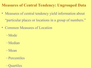
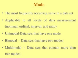
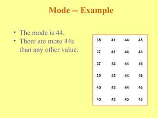
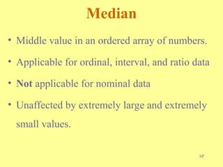
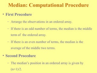
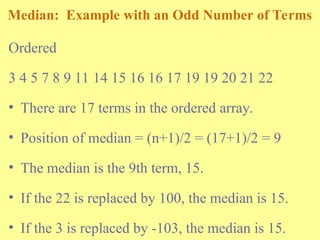
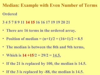
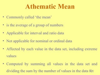
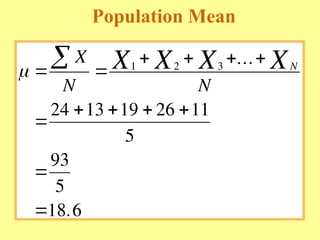
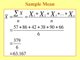
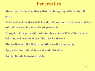
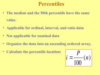
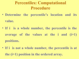
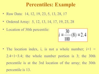
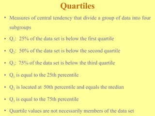
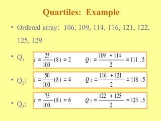
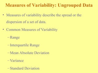
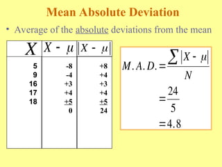
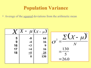
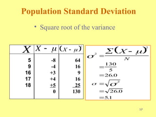
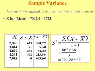
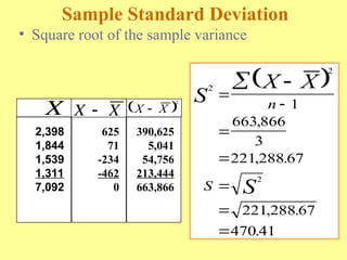
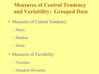
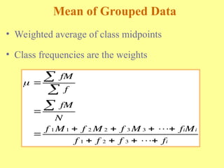
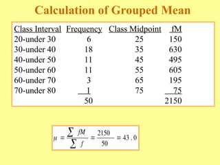
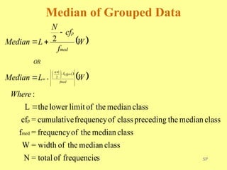
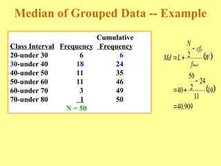
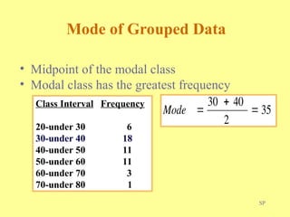
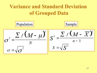
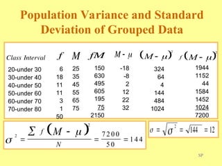
Chapter three discusses measures of central tendency and variability, focusing on ungrouped data. Key concepts include mode, median, mean, percentiles, and quartiles as measures of central location, as well as various measures of variability such as range and standard deviation. The chapter provides computational procedures and examples for understanding and calculating these statistical measures.

1. CHAPTER THREE
MEASURES OF CENTRAL
TENDENCY

2. Measures of Central Tendency: Ungrouped Data
• Measures of central tendency yield information about
“particular places or locations in a group of numbers.”
• Common Measures of Location
–Mode
–Median
–Mean
–Percentiles
–Quartiles

3. Mode
• The most frequently occurring value in a data set
• Applicable to all levels of data measurement
(nominal, ordinal, interval, and ratio)
• Unimodal-Data sets that have one mode
• Bimodal -- Data sets that have two modes
• Multimodal -- Data sets that contain more than
two modes

4. • The mode is 44.
• There are more 44s
than any other value.
35
37
37
39
40
40
41
41
43
43
43
43
44
44
44
44
44
45
45
46
46
46
46
48
Mode -- Example

5. SP
Median
• Middle value in an ordered array of numbers.
• Applicable for ordinal, interval, and ratio data
• Not applicable for nominal data
• Unaffected by extremely large and extremely
small values.

6. Median: Computational Procedure
• First Procedure
– Arrange the observations in an ordered array.
– If there is an odd number of terms, the median is the middle
term of the ordered array.
– If there is an even number of terms, the median is the
average of the middle two terms.
• Second Procedure
– The median’s position in an ordered array is given by
(n+1)/2.

7. Median: Example with an Odd Number of Terms
Ordered
3 4 5 7 8 9 11 14 15 16 16 17 19 19 20 21 22
• There are 17 terms in the ordered array.
• Position of median = (n+1)/2 = (17+1)/2 = 9
• The median is the 9th term, 15.
• If the 22 is replaced by 100, the median is 15.
• If the 3 is replaced by -103, the median is 15.

8. Median: Example with Even Number of Terms
Ordered
3 4 5 7 8 9 11 14 15 16 16 17 19 19 20 21
• There are 16 terms in the ordered array.
• Position of median = (n+1)/2 = (16+1)/2 = 8.5
• The median is between the 8th and 9th terms,
• Which is 14 +15/2 = 29/2 = 14.5.
• If the 21 is replaced by 100, the median is 14.5.
• If the 3 is replaced by -88, the median is 14.5.

9. SP
Athematic Mean
• Commonly called ‘the mean’
• is the average of a group of numbers
• Applicable for interval and ratio data
• Not applicable for nominal or ordinal data
• Affected by each value in the data set, including extreme
values
• Computed by summing all values in the data set and
dividing the sum by the number of values in the data set

10. Population Mean
  
   

   


 X
N N
X X X XN
1 2 3
24 13 19 26 11
5
93
5
18 6
...
.

11. Sample Mean
X
X
n n
X X X Xn
 
   

    


 1 2 3
57 86 42 38 90 66
6
379
6
63 167
...
.

12. SP
Percentiles
• Measures of central tendency that divide a group of data into 100
parts
• At least n% of the data lie below the nth percentile, and at most (100 -
n)% of the data lie above the nth percentile
• Example: 90th percentile indicates that at least 90% of the data lie
below it, and at most 10% of the data lie above it
• The median and the 50th percentile have the same value.
• Applicable for ordinal, interval, and ratio data
• Not applicable for nominal data

13. Percentiles
• The median and the 50th percentile have the same
value.
• Applicable for ordinal, interval, and ratio data
• Not applicable for nominal data
• Organize the data into an ascending ordered array.
• Calculate the percentile location:
i
P
n

100
( )

14. Percentiles: Computational
Procedure
• Determine the percentile’s location and its
value.
• If i is a whole number, the percentile is the
average of the values at the i and (i+1)
positions.
• If i is not a whole number, the percentile is at
the (i+1) position in the ordered array.

15. Percentiles: Example
• Raw Data: 14, 12, 19, 23, 5, 13, 28, 17
• Ordered Array: 5, 12, 13, 14, 17, 19, 23, 28
• Location of 30th percentile:
• The location index, i, is not a whole number; i+1 =
2.4+1=3.4; the whole number portion is 3; the 30th
percentile is at the 3rd location of the array; the 30th
percentile is 13.
i  
30
100
8 2 4
( ) .

16. Quartiles
• Measures of central tendency that divide a group of data into four
subgroups
• Q1: 25% of the data set is below the first quartile
• Q2: 50% of the data set is below the second quartile
• Q3: 75% of the data set is below the third quartile
• Q1 is equal to the 25th percentile
• Q2 is located at 50th percentile and equals the median
• Q3 is equal to the 75th percentile
• Quartile values are not necessarily members of the data set

17. • Ordered array: 106, 109, 114, 116, 121, 122,
125, 129
• Q1
• Q2:
• Q3:
Quartiles: Example
i Q
  


25
100
8 2
109 114
2
111 5
1
( ) .
i Q
  


50
100
8 4
116 121
2
118 5
2
( ) .
i Q
  


75
100
8 6
122 125
2
123 5
3
( ) .

18. Measures of Variability: Ungrouped Data
• Measures of variability describe the spread or the
dispersion of a set of data.
• Common Measures of Variability
–Range
–Interquartile Range
–Mean Absolute Deviation
–Variance
–Standard Deviation

19. Range
• The difference between the largest and the smallest
values in a set of data
• Simple to compute
• Ignores all data points except
the two extremes
• Example:
• Range = Largest – Smallest = 48 - 35 = 13
35
37
37
39
40
40
41
41
43
43
43
43
44
44
44
44
44
45
45
46
46
46
46
48

20. Interquartile Range
• Range of values between the first and third
quartiles
• Range of the “middle half”
• Less influenced by extremes
Interquartile Range Q Q
 
3 1

21. Deviation from the Mean
• Data set: 5, 9, 16, 17, 18
• Mean:
• Deviations from the mean: -8, -4, 3, 4, 5
   
 X
N
65
5
13
0 5 10 15 20
-8
-4
+3
+4
+5


22. Mean Absolute Deviation
• Average of the absolute deviations from the mean
5
9
16
17
18
-8
-4
+3
+4
+5
0
+8
+4
+3
+4
+5
24
X X   X  
M A D
X
N
. . .
.




 
24
5
4 8

23. Population Variance
• Average of the squared deviations from the arithmetic mean
5
9
16
17
18
-8
-4
+3
+4
+5
0
64
16
9
16
25
130
X X    
2
X  
 
2
2
130
5
26 0






 X
N
.

24. SP
Population Standard Deviation
• Square root of the variance
 
2
2
2
130
5
26 0
26 0
51











 X
N
.
.
.
5
9
16
17
18
-8
-4
+3
+4
+5
0
64
16
9
16
25
130
X X    
2
X  

25. Sample Variance
• Average of the squared deviations from the arithmetic mean
• X-bar (Mean) = 7092/4 = 1773
2,398
1,844
1,539
1,311
7,092
625
71
-234
-462
0
390,625
5,041
54,756
213,444
663,866
X X X
  
2
X X

 
2
2
1
663 866
3
221 288 67
S
X X
n






,
, .

26. Sample Standard Deviation
• Square root of the sample variance
 
2
2
2
1
663 866
3
221 288 67
221 288 67
470 41
S
X X
S
n
S









,
, .
, .
.
2,398
1,844
1,539
1,311
7,092
625
71
-234
-462
0
390,625
5,041
54,756
213,444
663,866
X X X
  
2
X X


27. Measures of Central Tendency
and Variability: Grouped Data
• Measures of Central Tendency
–Mean
–Median
–Mode
• Measures of Variability
–Variance
–Standard Deviation

28. Mean of Grouped Data
• Weighted average of class midpoints
• Class frequencies are the weights
 


   



   






fM
f
fM
N
f M f M f M f M
f f f f
i i
i
1 1 2 2 3 3
1 2 3

29. Calculation of Grouped Mean
Class Interval Frequency Class Midpoint fM
20-under 30 6 25 150
30-under 40 18 35 630
40-under 50 11 45 495
50-under 60 11 55 605
60-under 70 3 65 195
70-under 80 1 75 75
50 2150
   


fM
f
2150
50
43 0
.

30. SP
Median of Grouped Data
 
 
 
s
frequencie
of
total
=
N
class
median
the
of
width
=
W
class
median
the
of
frequency
=
f
class
median
the
preceding
class
of
frequency
cumulative
=
cf
class
median
the
of
limit
lower
the
L
:
2
med
p
1
2
1
























 

Where
W
L
Median
W
f
cf
N
L
Median
fmed
cfp
n
m
OR
med
p

31. Median of Grouped Data -- Example
Cumulative
Class Interval Frequency Frequency
20-under 30 6 6
30-under 40 18 24
40-under 50 11 35
50-under 60 11 46
60-under 70 3 49
70-under 80 1 50
N = 50
 
 
909
.
40
10
11
24
2
50
40
2






 W
f
cf
N
L
Md
med
p

32. SP
Mode of Grouped Data
• Midpoint of the modal class
• Modal class has the greatest frequency
Class Interval Frequency
20-under 30 6
30-under 40 18
40-under 50 11
50-under 60 11
60-under 70 3
70-under 80 1
Mode 


30 40
2
35

33. SP
Variance and Standard Deviation
of Grouped Data
 
2
2
2







 f
N
M
Population
 
2
2
2
1
S
M X
S
f
n
S





Sample

34. SP
Population Variance and Standard
Deviation of Grouped Data
1944
1152
44
1584
1452
1024
7200
20-under 30
30-under 40
40-under 50
50-under 60
60-under 70
70-under 80
Class Interval
6
18
11
11
3
1
50
f
25
35
45
55
65
75
M
150
630
495
605
195
75
2150
fM
-18
-8
2
12
22
32
M    
f M
2
 
324
64
4
144
484
1024
 
2
M  
 
2
2
7 2 0 0
5 0
1 4 4


  

 f
N
M  
  
2
144 12

35. SP
Measures of Shape
• Skewness
– Absence of symmetry
– Extreme values in one side of a distribution
• Kurtosis
– Peakedness of a distribution
– Leptokurtic: high and thin
– Mesokurtic: normal shape
– Platykurtic: flat and spread out

36. Skewness
Negatively
Skewed
Mode
Median
Mean
Symmetric
(Not Skewed)
Mean
Median
Mode
Positively
Skewed
Mode
Median
Mean

37. 3-37
Kurtosis
• Peakedness of a distribution
– Leptokurtic: high and thin
– Mesokurtic: normal in shape
– Platykurtic: flat and spread out
Leptokurtic
Mesokurtic
Platykurtic