Splay trees are self-balancing binary search trees that provide fast access both in worst-case amortized time (O(log n)) and in practice due to their locality properties. When a node is accessed, it is rotated to the root through a series of zig-zag and zig-zig rotations, improving locality for future accesses. This helps frequently accessed nodes rise to the top of the tree over time. Splay trees also support efficient split and join operations through splaying, which makes them useful for tasks like range queries and dictionary operations.

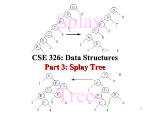
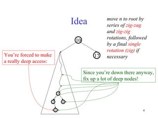
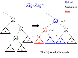
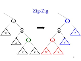
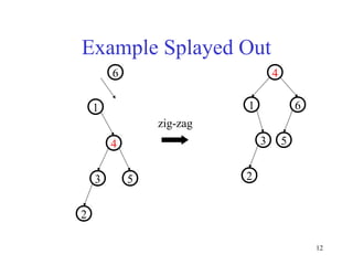
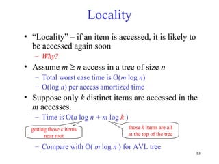
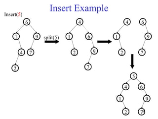
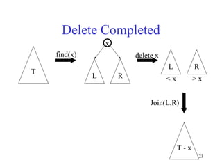
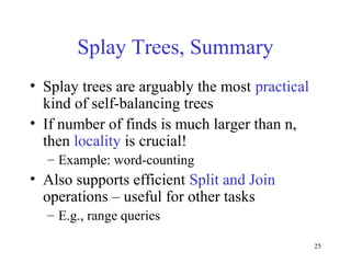
1. 1
Splay
Trees
CSE 326: Data StructuresCSE 326: Data Structures
Part 3: Splay TreePart 3: Splay Tree

2. 2
Today: Splay Trees
• Fast both in worst-case amortized analysis
and in practice
• Are used in the kernel of NT for keep track of
process information!
• Invented by Sleator and Tarjan (1985)
• Details:
• Weiss 4.5 (basic splay trees)
• 11.5 (amortized analysis)
• 12.1 (better “top down” implementation)

3. 3
Basic Idea
“Blind” rebalancing – no height info kept!
• Worst-case time per operation is O(n)
• Worst-case amortized time is O(log n)
• Insert/find always rotates node to the root!
• Good locality:
– Most commonly accessed keys move high in
tree – become easier and easier to find

4. 4
Idea
17
10
92
5
3
You’re forced to make
a really deep access:
Since you’re down there anyway,
fix up a lot of deep nodes!
move n to root by
series of zig-zag
and zig-zig
rotations, followed
by a final single
rotation (zig) if
necessary

5. 5
Zig-Zag*
g
X
p
Y
n
Z
W
*
This is just a double rotation
n
Y
g
W
p
ZX
Helped
Unchanged
Hurt
up 2
down 1
up 1down 1

6. 6
Zig-Zig
n
Z
Y
p
X
g
W
g
W
X
p
Y
n
Z

7. 7
Why Splaying Helps
• Node n and its children are always helped (raised)
• Except for last step, nodes that are hurt by a zig-
zag or zig-zig are later helped by a rotation higher
up the tree!
• Result:
– shallow nodes may increase depth by one or two
– helped nodes decrease depth by a large amount
• If a node n on the access path is at depth d before
the splay, it’s at about depth d/2 after the splay
– Exceptions are the root, the child of the root, and the
node splayed

8. 8
Splaying Example
2
1
3
4
5
6
Find(6)
2
1
3
6
5
4
zig-zig

9. 9
Still Splaying 6
zig-zig
2
1
3
6
5
4
1
6
3
2 5
4

10. 10
Almost There, Stay on Target
zig
1
6
3
2 5
4
6
1
3
2 5
4

11. 11
Splay Again
Find(4)
zig-zag
6
1
3
2 5
4
6
1
4
3 5
2

12. 12
Example Splayed Out
zig-zag
6
1
4
3 5
2
61
4
3 5
2

13. 13
Locality
• “Locality” – if an item is accessed, it is likely to
be accessed again soon
– Why?
• Assume m ≥ n access in a tree of size n
– Total worst case time is O(m log n)
– O(log n) per access amortized time
• Suppose only k distinct items are accessed in the
m accesses.
– Time is O(n log n + m log k )
– Compare with O( m log n ) for AVL tree
getting those k items
near root
those k items are all
at the top of the tree

14. 14
Splay Operations: Insert
• To insert, could do an ordinary BST insert
– but would not fix up tree
– A BST insert followed by a find (splay)?
• Better idea: do the splay before the insert!
• How?

15. 15
Split
Split(T, x) creates two BST’s L and R:
– All elements of T are in either L or R
– All elements in L are ≤ x
– All elements in R are ≥ x
– L and R share no elements
Then how do we do the insert?

16. 16
Split
Split(T, x) creates two BST’s L and R:
– All elements of T are in either L or R
– All elements in L are ≤ x
– All elements in R are > x
– L and R share no elements
Then how do we do the insert?
Insert as root, with children L and R

17. 17
Splitting in Splay Trees
• How can we split?
– We have the splay operation
– We can find x or the parent of where x would
be if we were to insert it as an ordinary BST
– We can splay x or the parent to the root
– Then break one of the links from the root to a
child

18. 18
Split
split(x)
T L R
splay
OR
L R L R
≤ x > x> x < x
could be x, or
what would
have been the
parent of x
if root is ≤ x
if root is > x

19. 19
Back to Insert
split(x)
L R
x
L R
> x≤ x
Insert(x):
Split on x
Join subtrees using x as root

20. 20
Insert Example
91
6
4 7
2
Insert(5)
split(5)
9
6
7
1
4
2
1
4
2
9
6
7
1
4
2
9
6
7
5

21. 21
Splay Operations: Delete
find(x)
L R
x
L R
> x< x
delete x
Now what?

22. 22
Join
• Join(L, R): given two trees such that L < R,
merge them
• Splay on the maximum element in L then
attach R
L R R
splay L

23. 23
Delete Completed
T
find(x)
L R
x
L R
> x< x
delete x
T - x
Join(L,R)

24. 24
Delete Example
91
6
4 7
2
Delete(4)
find(4)
9
6
7
1
4
2
1
2
9
6
7
Find max
2
1
9
6
7
2
1
9
6
7

25. 25
Splay Trees, Summary
• Splay trees are arguably the most practical
kind of self-balancing trees
• If number of finds is much larger than n,
then locality is crucial!
– Example: word-counting
• Also supports efficient Split and Join
operations – useful for other tasks
– E.g., range queries