Download to read offline


![Empty Heap Creation
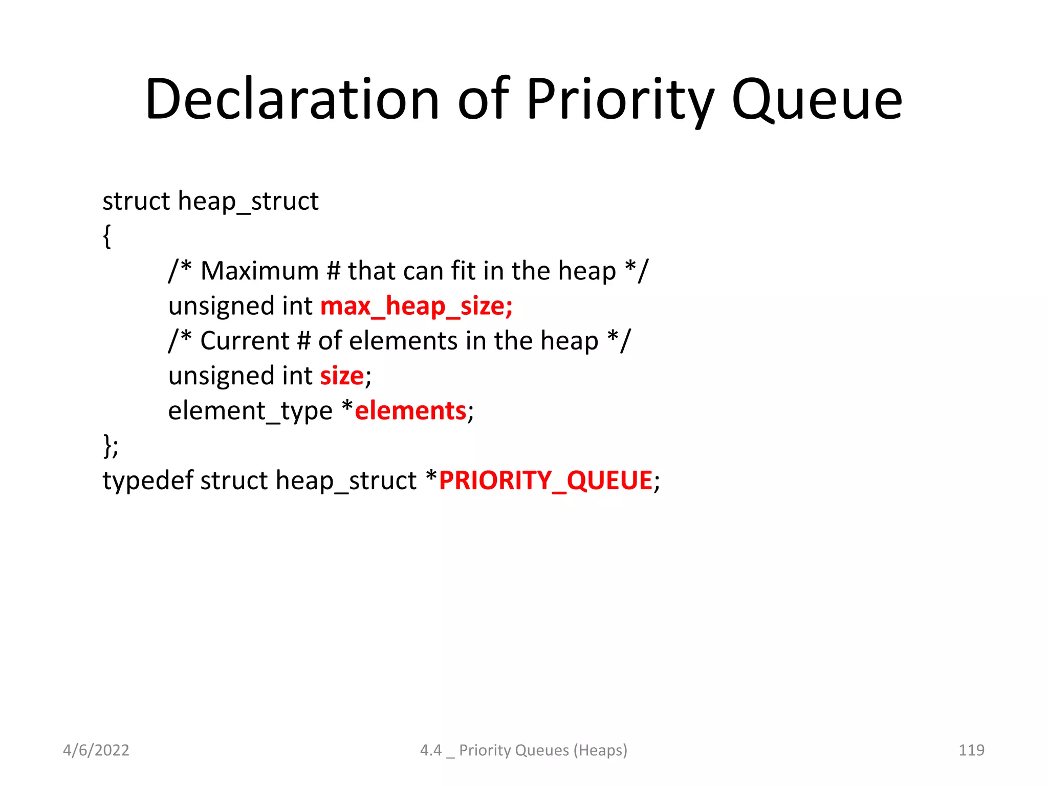
PRIORITY_QUEUE create_pq( unsigned int max_elements )
{
PRIORITY_QUEUE H;
if( max_elements < MIN_PQ_SIZE )
error("Priority queue size is too small");
H = (PRIORITY_QUEUE) malloc ( sizeof (struct heap_struct) );
if( H == NULL )
fatal_error("Out of space!!!");
/* Allocate the array + one extra for sentinel */
H->elements = (element_type *) malloc ( ( max_elements+1) * sizeof (element_type) );
if( H->elements == NULL )
fatal_error("Out of space!!!");
H->max_heap_size = max_elements;
H->size = 0;
H->elements[0] = MIN_DATA;
return H;
}
4/6/2022 4.4 _ Priority Queues (Heaps) 120](https://image.slidesharecdn.com/unit4complete-211228094050/75/Advanced-Trees-118-2048.jpg)
![Insertion - Code
/* H->element[0] is a sentinel */
Void insert( element_type x, PRIORITY_QUEUE H )
{
unsigned int i;
if( is_full( H ) )
error("Priority queue is full");
else
{
i = ++H->size;
while( H->elements[i/2] > x )
{
H->elements[i] = H->elements[i/2];
i /= 2;
}
H->elements[i] = x;
}
}
4/6/2022 4.4 _ Priority Queues (Heaps) 128](https://image.slidesharecdn.com/unit4complete-211228094050/75/Advanced-Trees-126-2048.jpg)

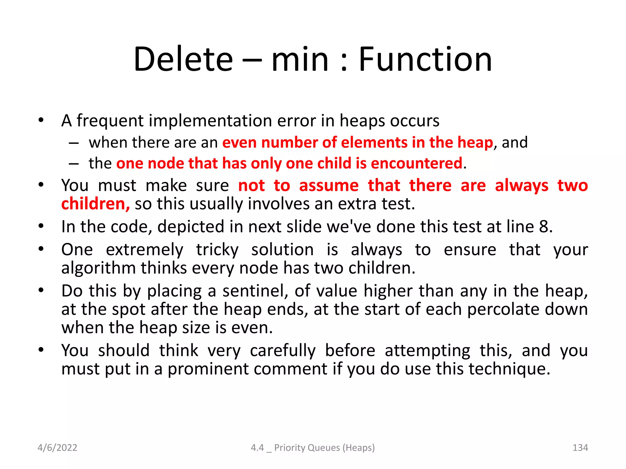
![Delete _ min : function
• element_type Delete_min( PRIORITY_QUEUE H )
• {
• unsigned int i, child;
• element_type min_element, last_element;
• if( is_empty( H ) )
• {
• error("Priority queue is empty");
• return H->elements[0];
• }
• min_element = H->elements[1];
• last_element = H->elements[H->size--];
• for( i=1; i*2 <= H->size; i=child )
• {
• /* find smaller child */
• child = i*2;
• if( ( child != H->size ) && ( H->elements[child+1] < H->elements [child] ) ) // LINE 8
• child++;
• /* percolate one level */
• if( last_element > H->elements[child] )
• H->elements[i] = H->elements[child];
• Else
• break;
• }
• H->elements[i] = last_element;
• return min_element;
• }
4/6/2022 4.4 _ Priority Queues (Heaps) 135](https://image.slidesharecdn.com/unit4complete-211228094050/75/Advanced-Trees-133-2048.jpg)


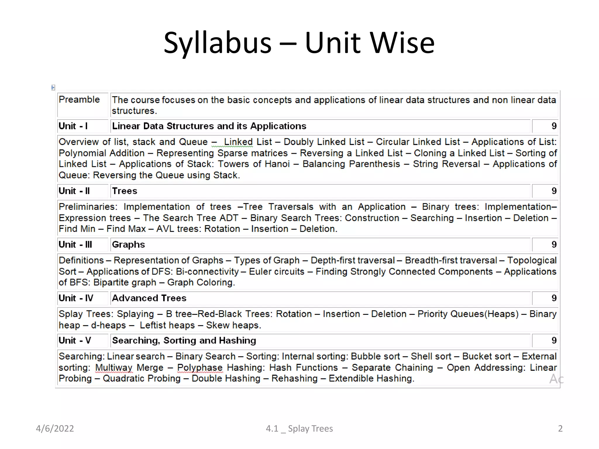
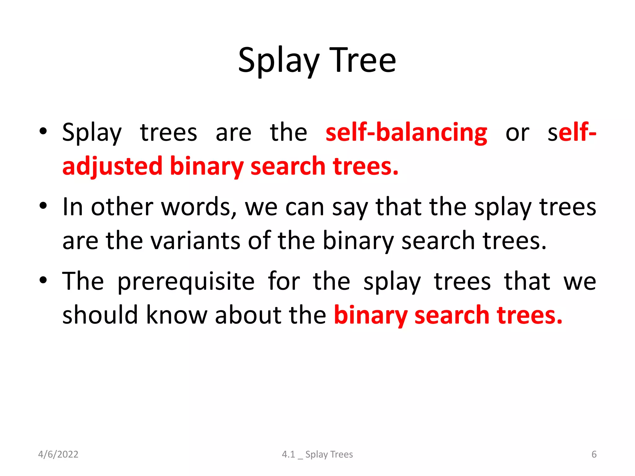
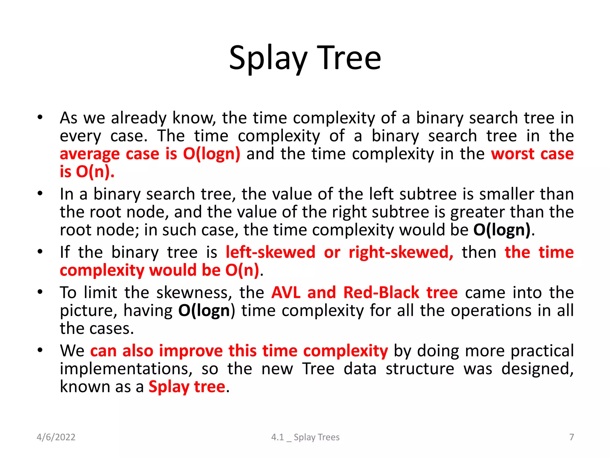
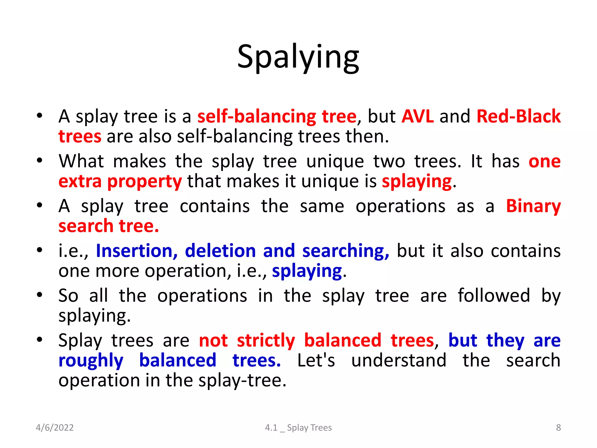
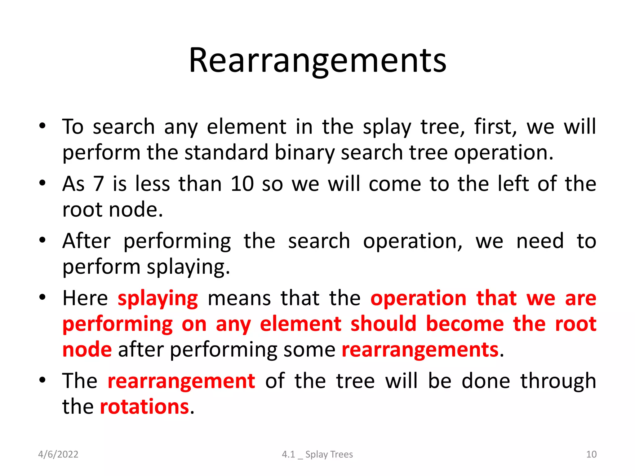
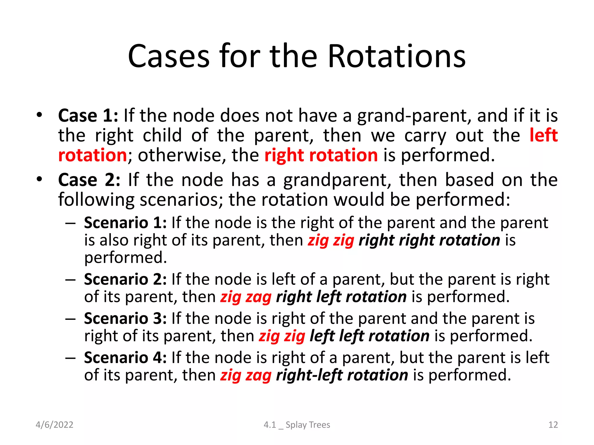
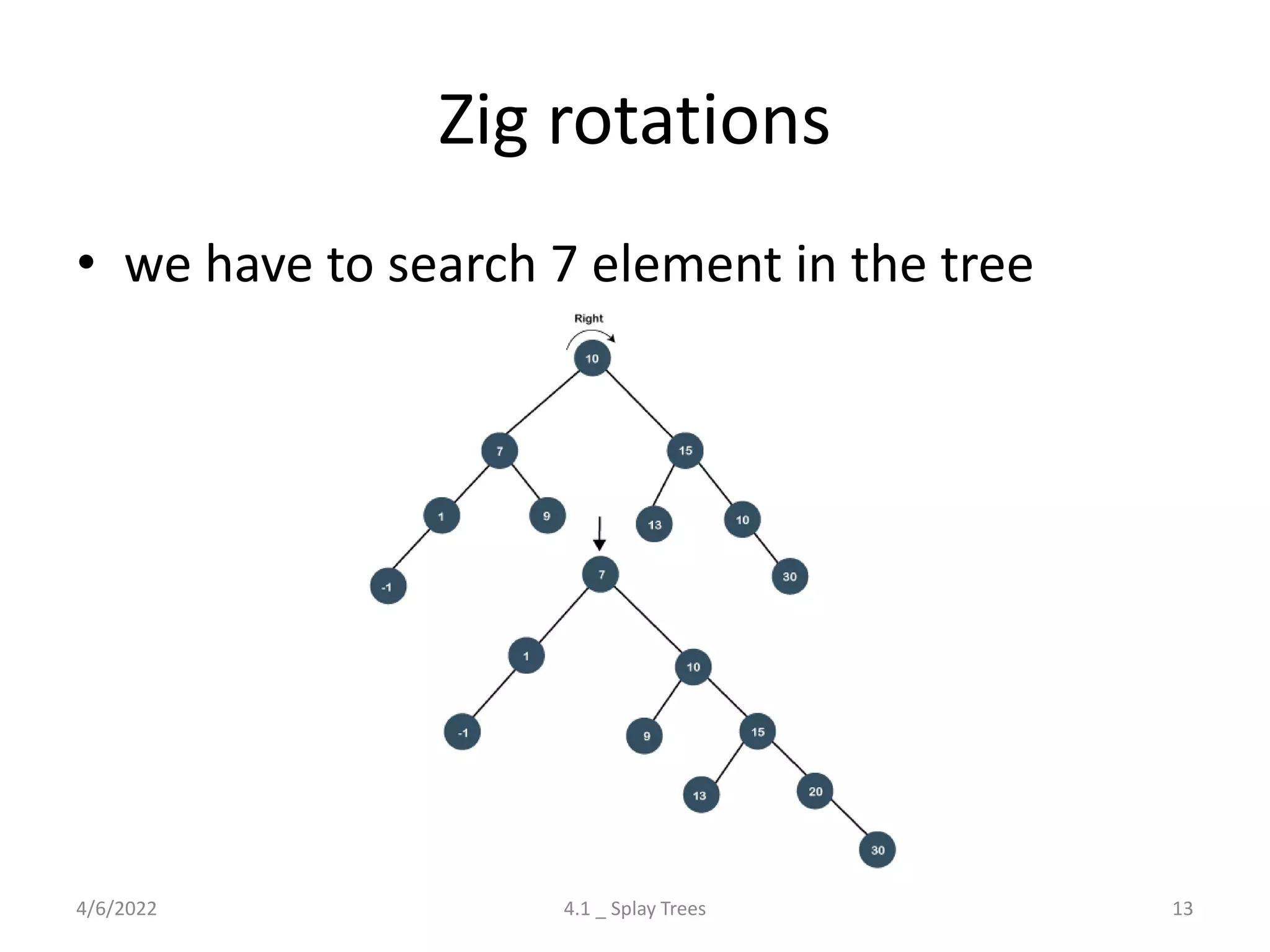
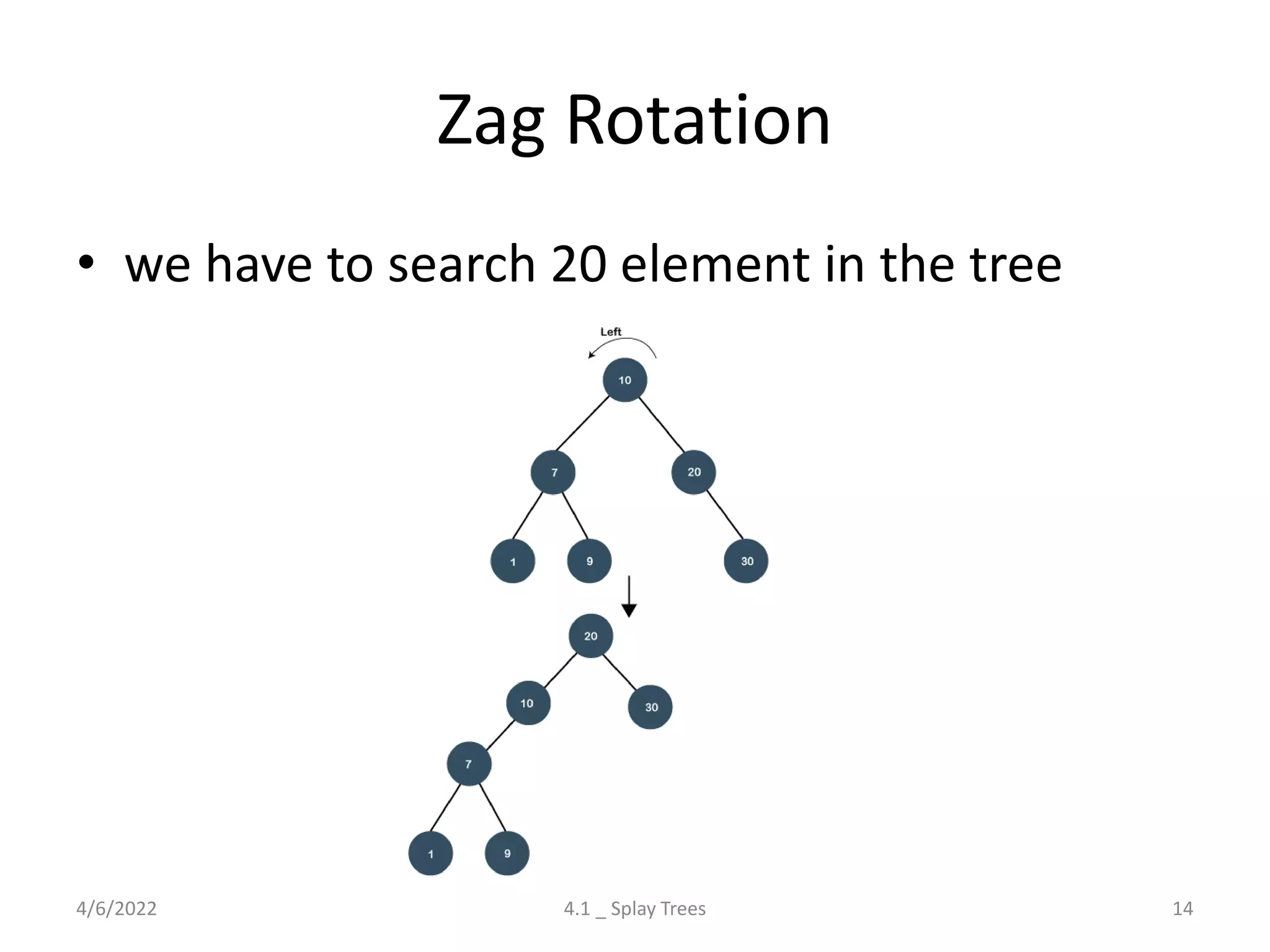
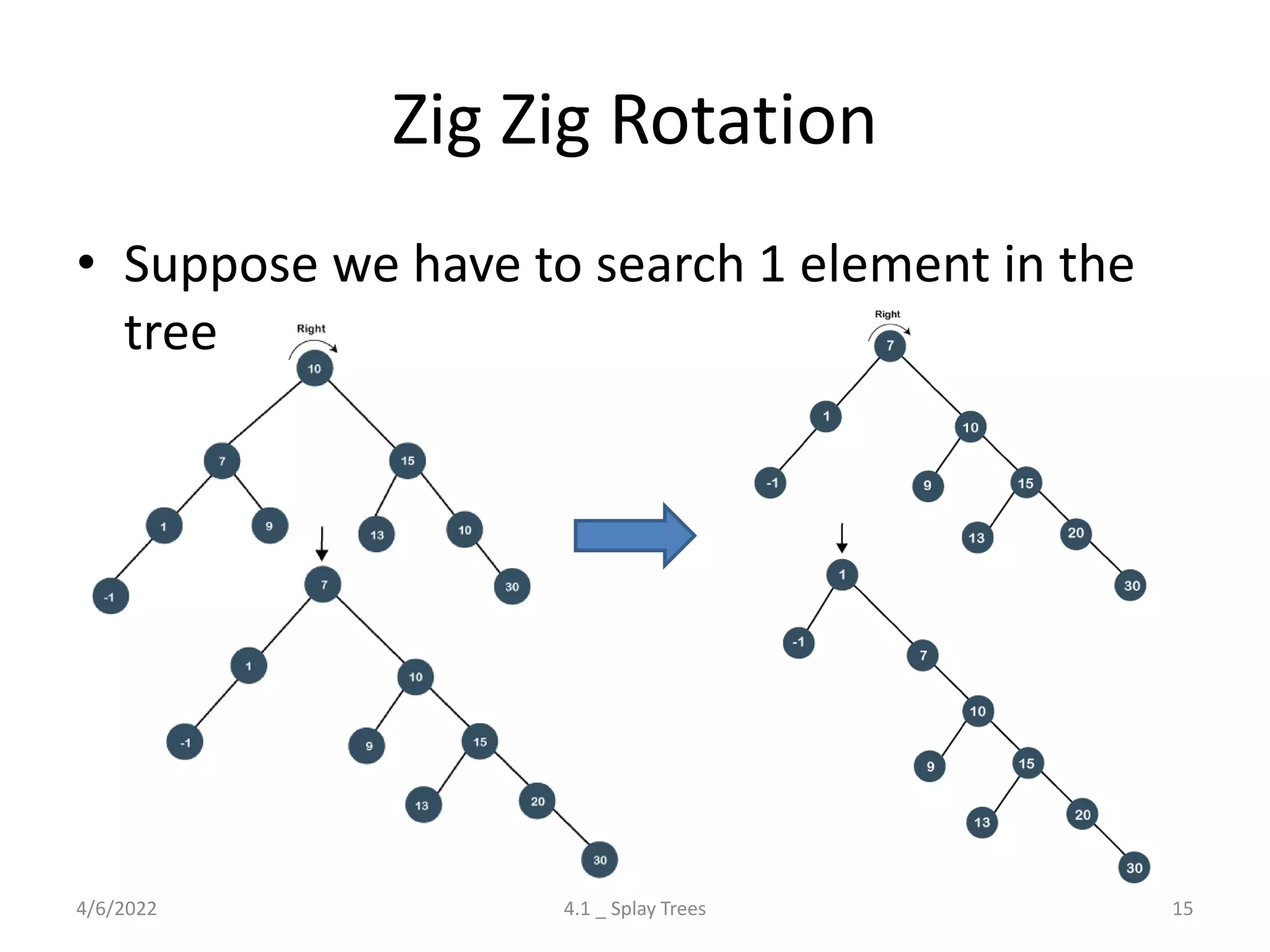
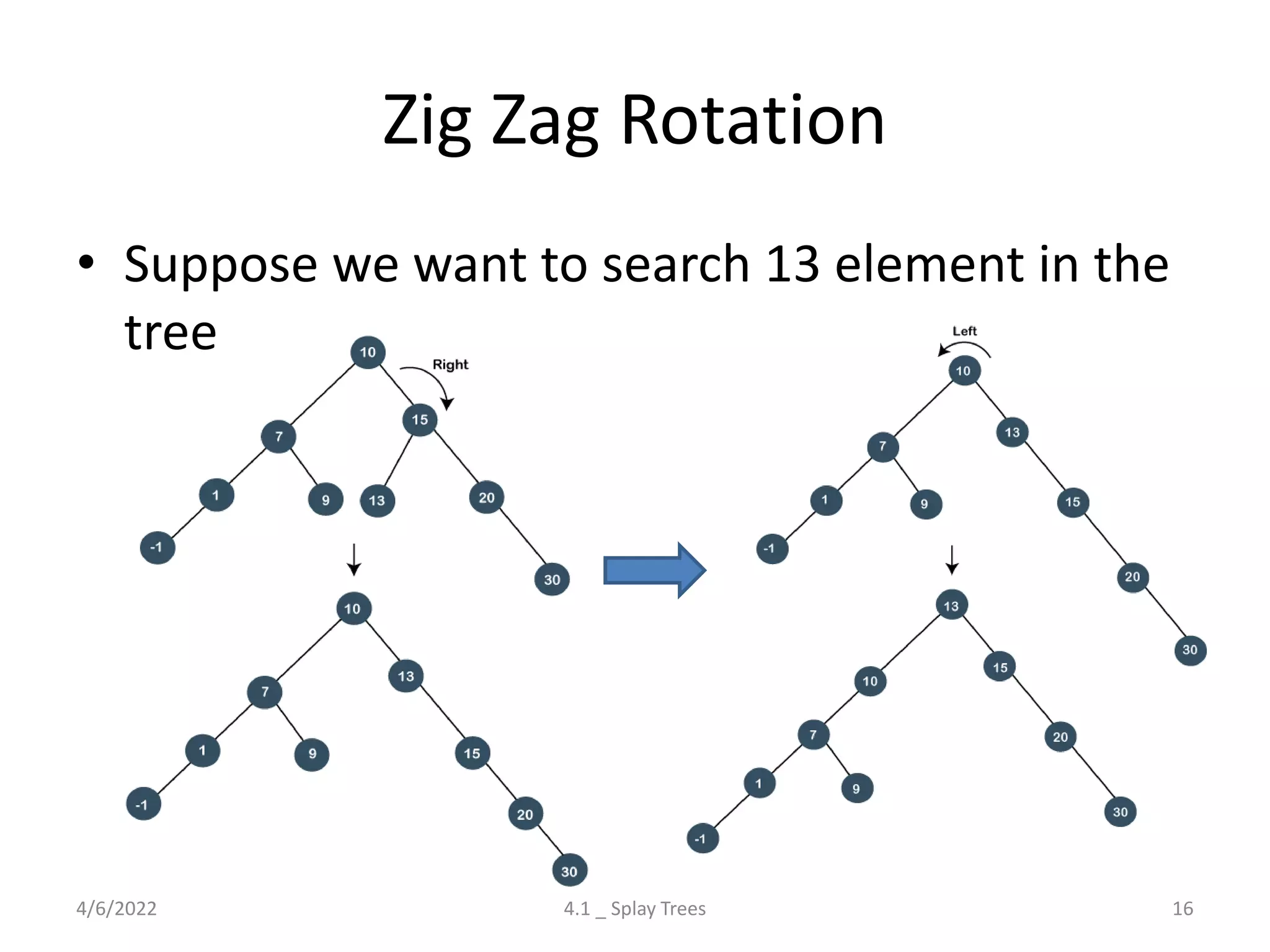
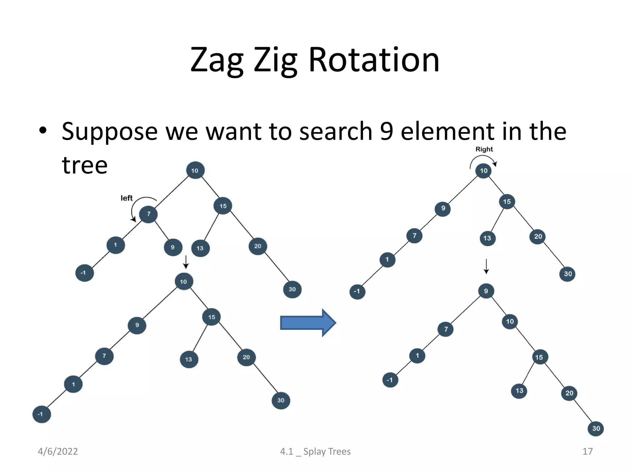
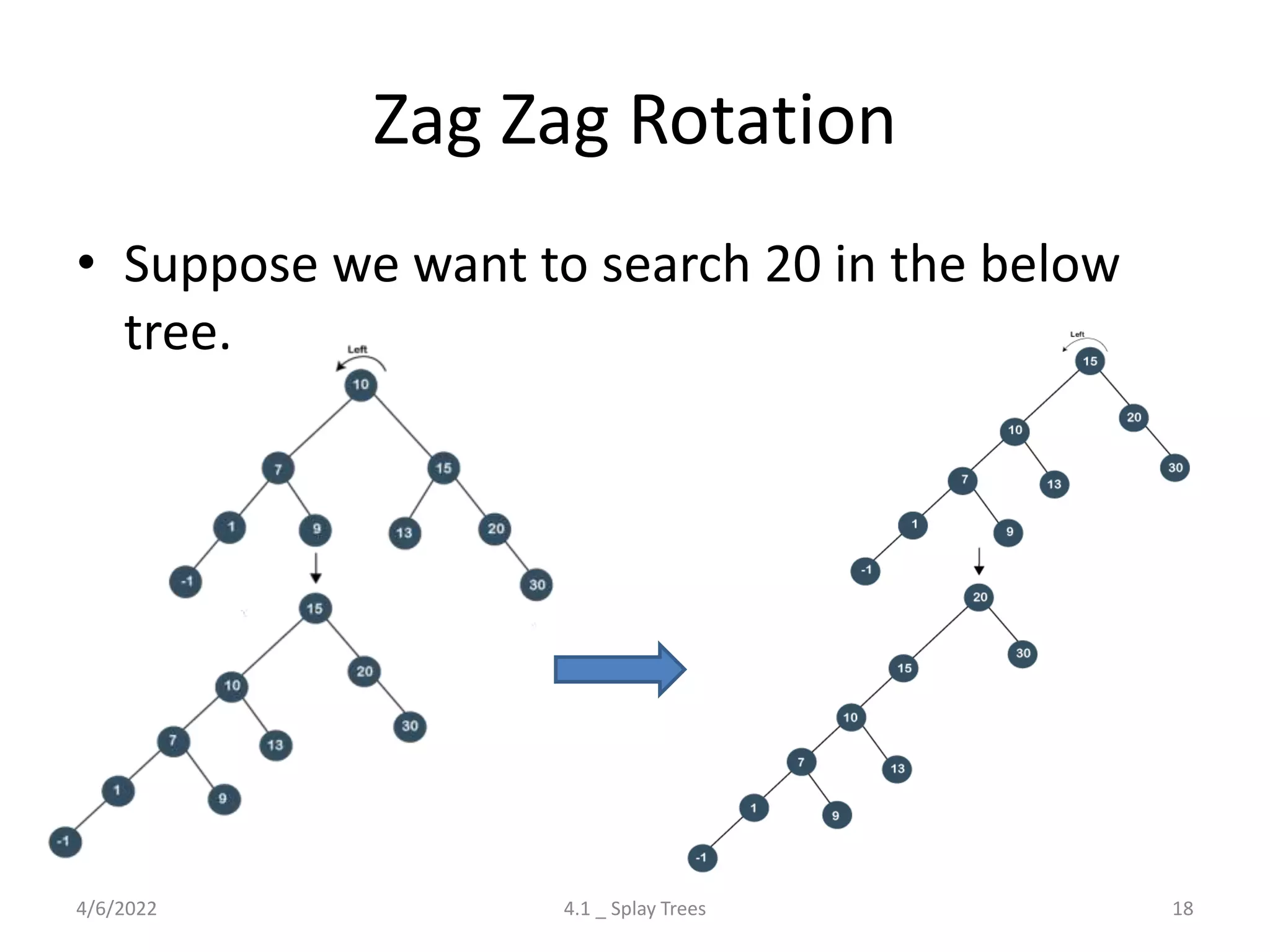
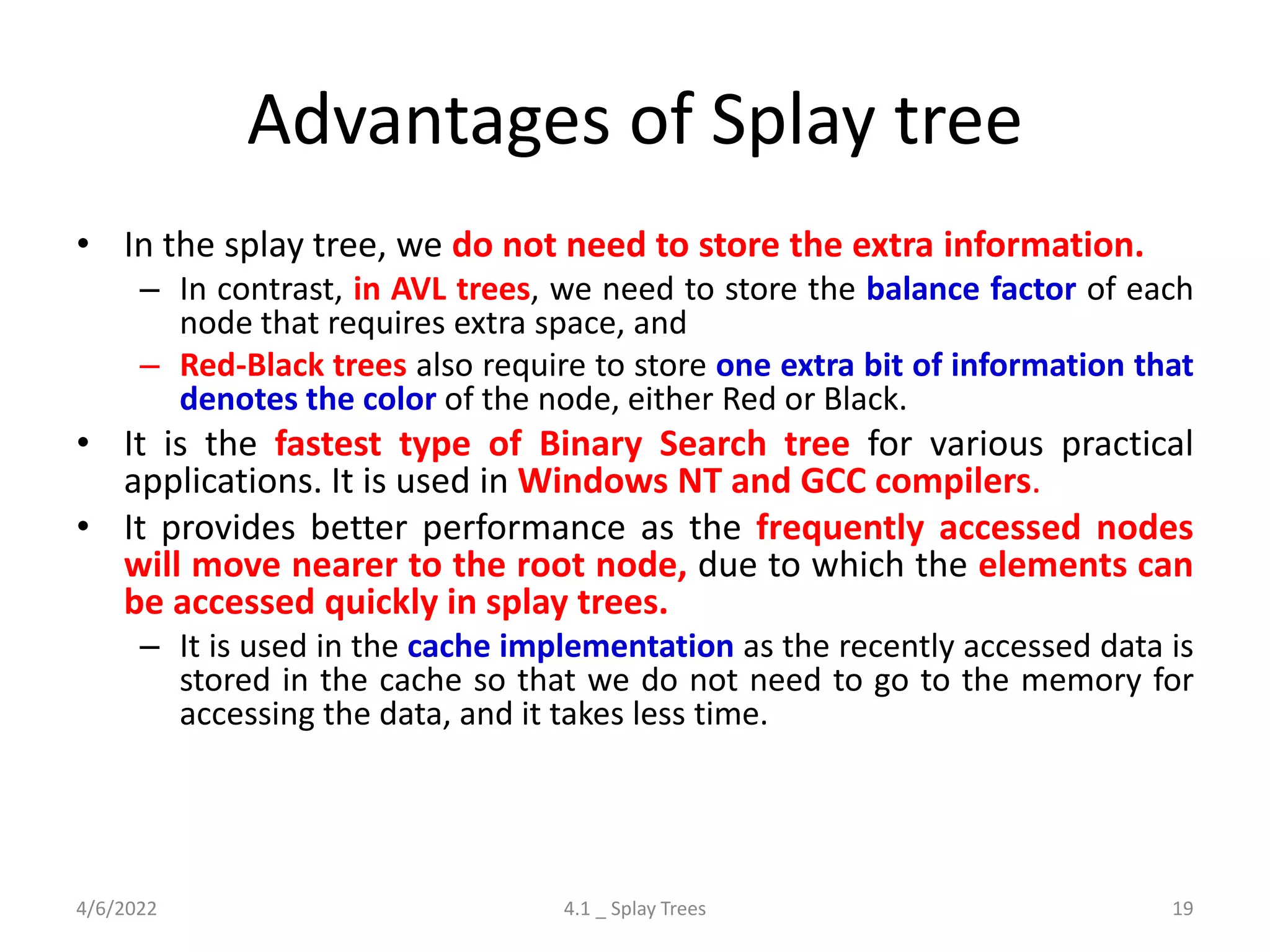
The document discusses splay trees, which are self-balancing binary search trees where frequently accessed nodes are moved closer to the root through rotations. It covers the different types of rotations used in splay trees - zig, zag, zig-zig, zig-zag, zag-zig, and zag-zag. Examples of searching elements and performing the necessary rotations on a splay tree are provided. Advantages of splay trees include not requiring extra space for balance factors, while a drawback is they are only roughly balanced rather than strictly balanced like AVL or red-black trees.
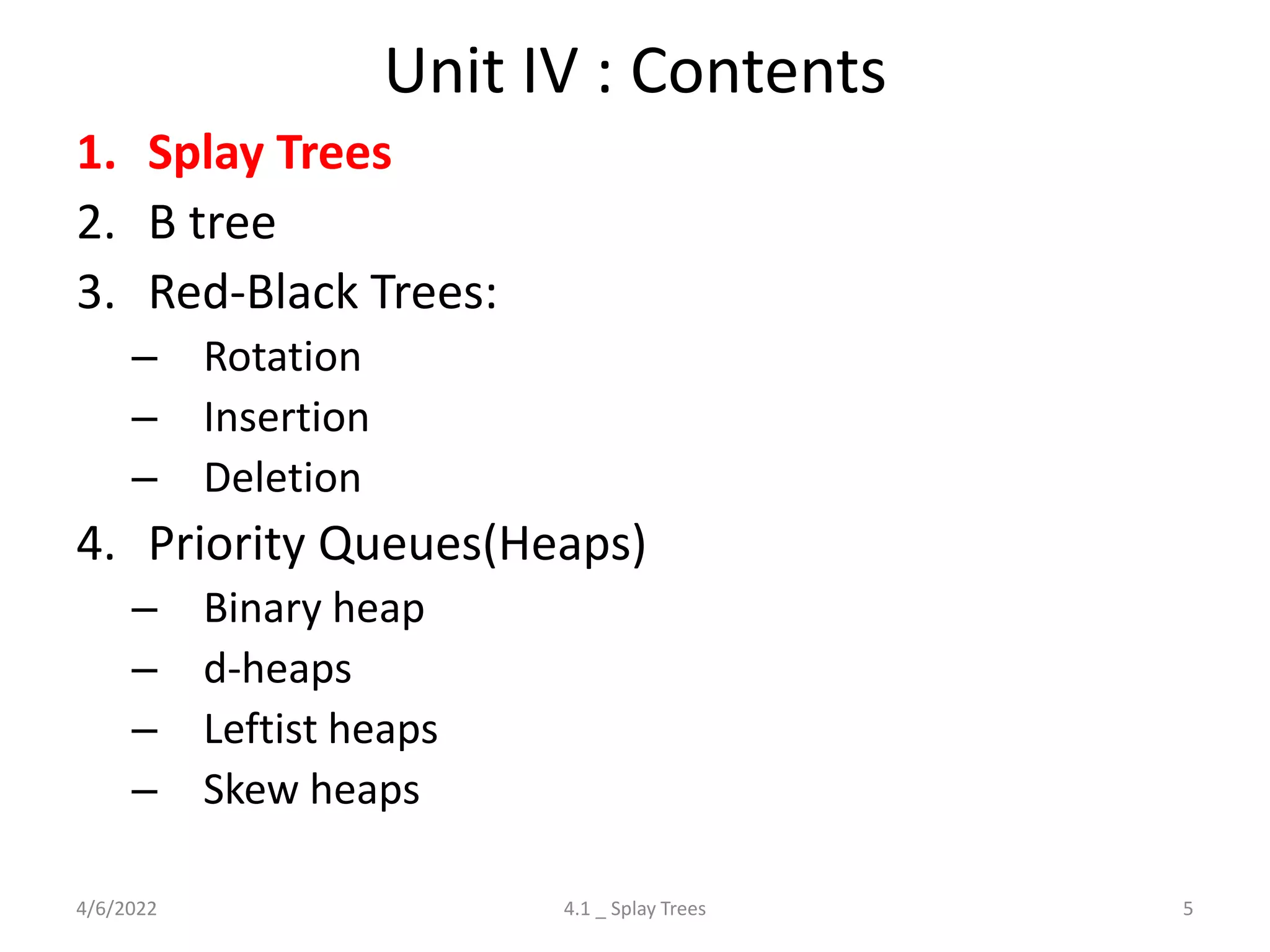
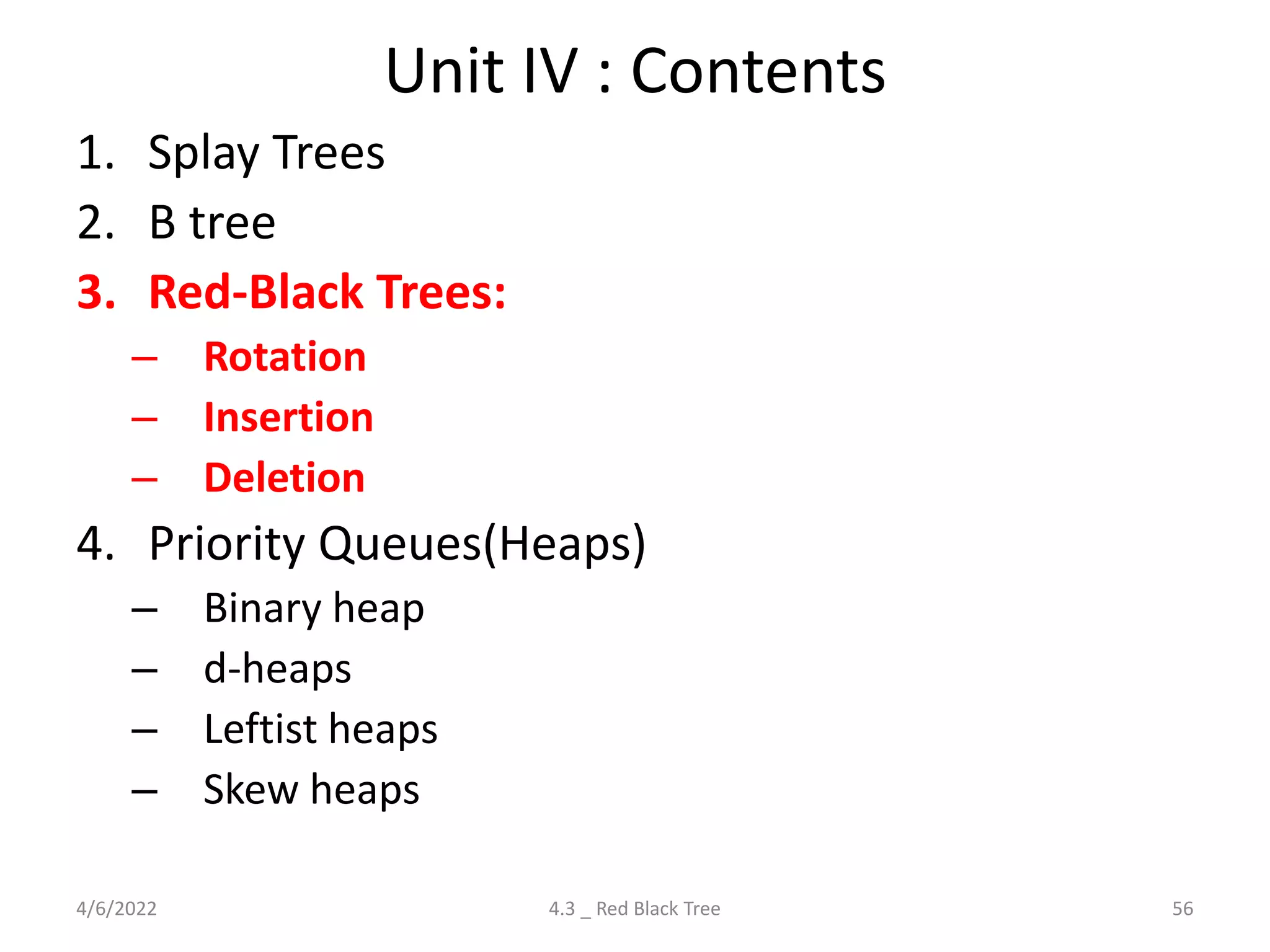
Introduction to Advanced Trees covering Splay Trees, B tree, Red-Black Trees, and Priority Queues.
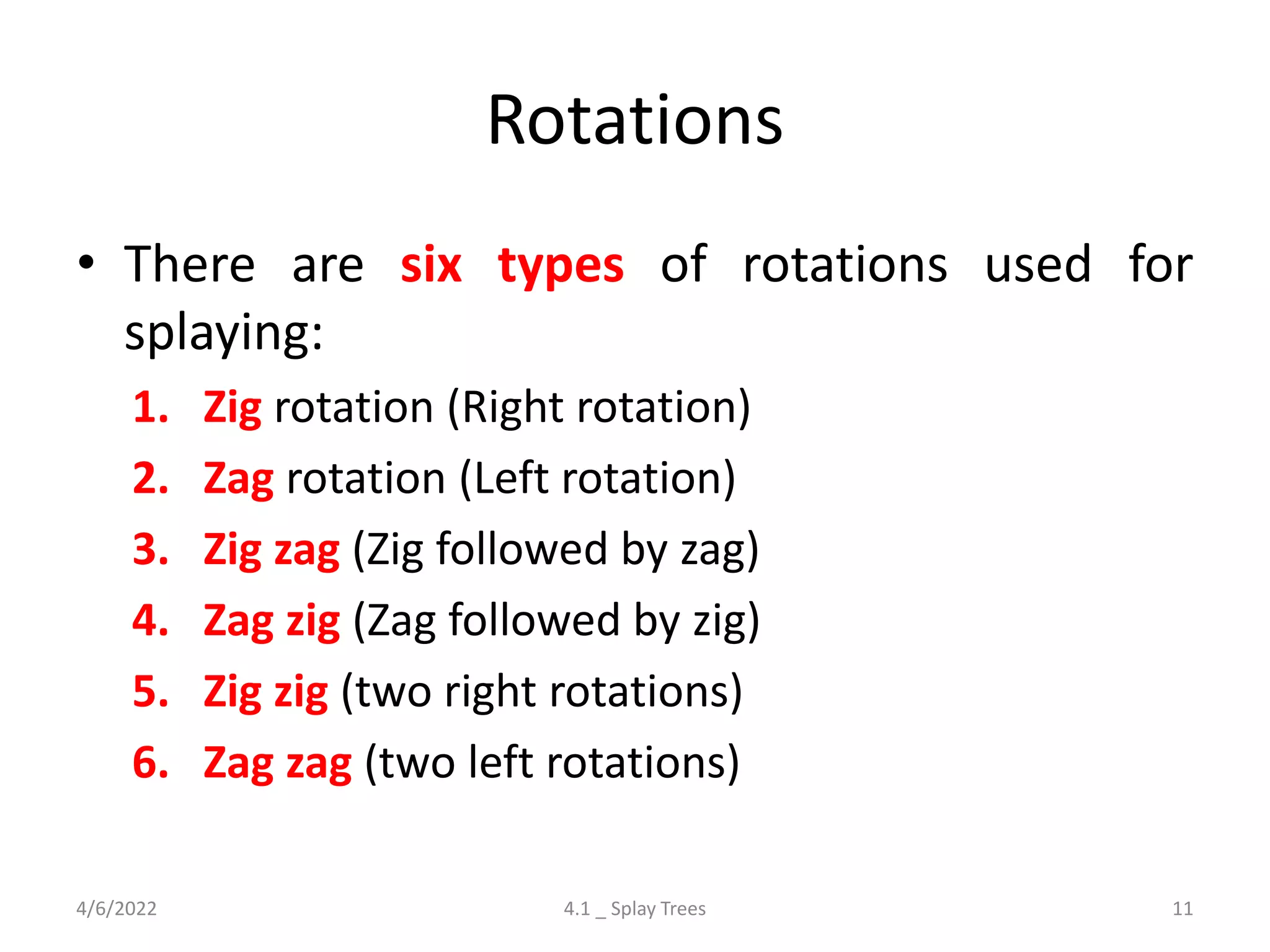
Discussion on Splay Trees: their properties, rotations (Zig, Zag), time complexities, advantages, and drawbacks.
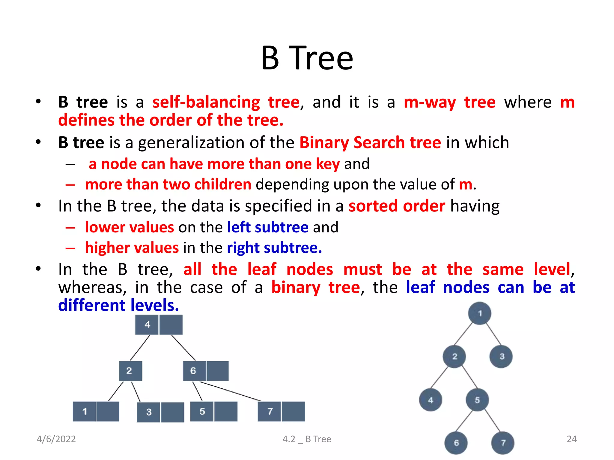
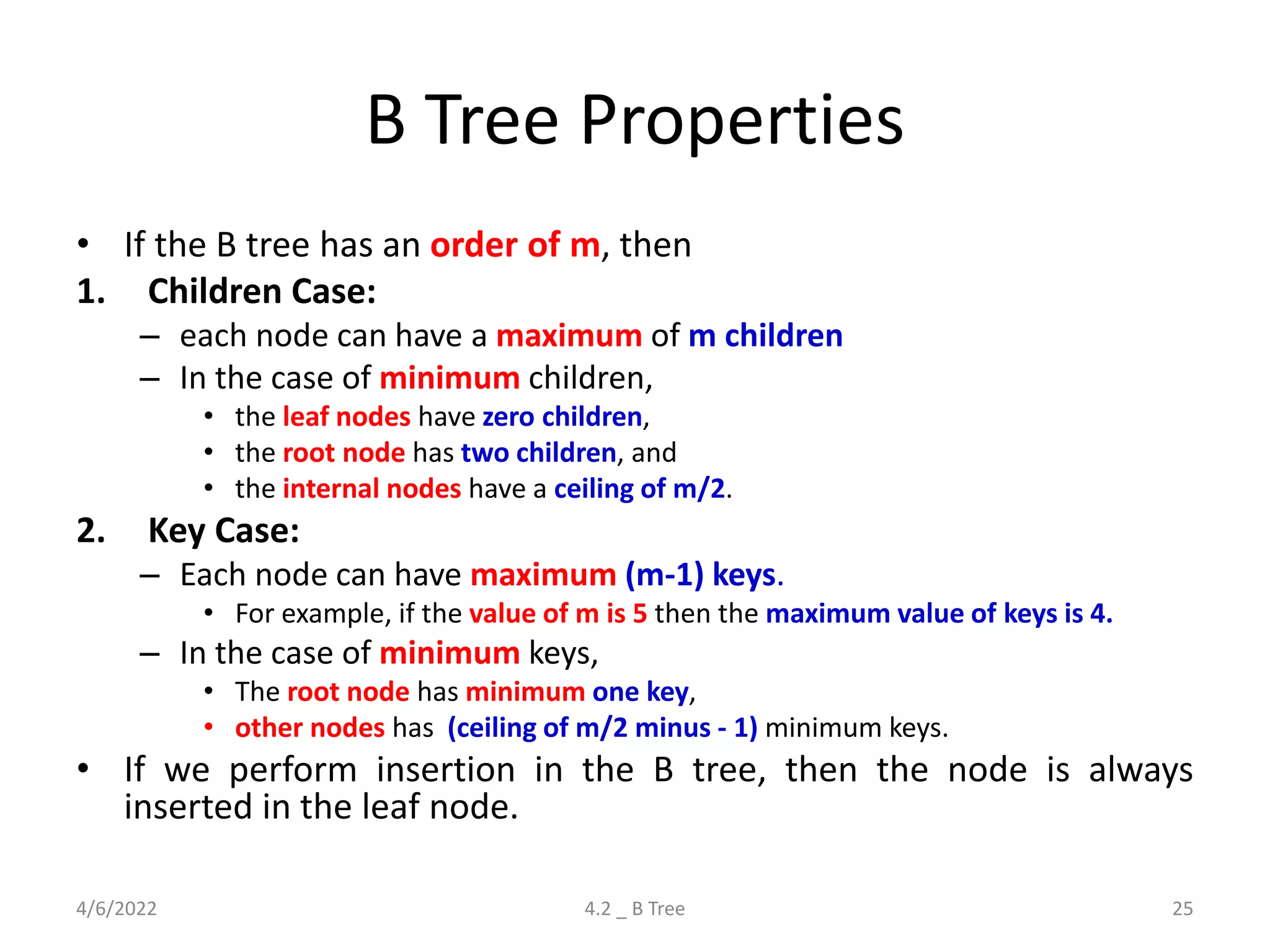
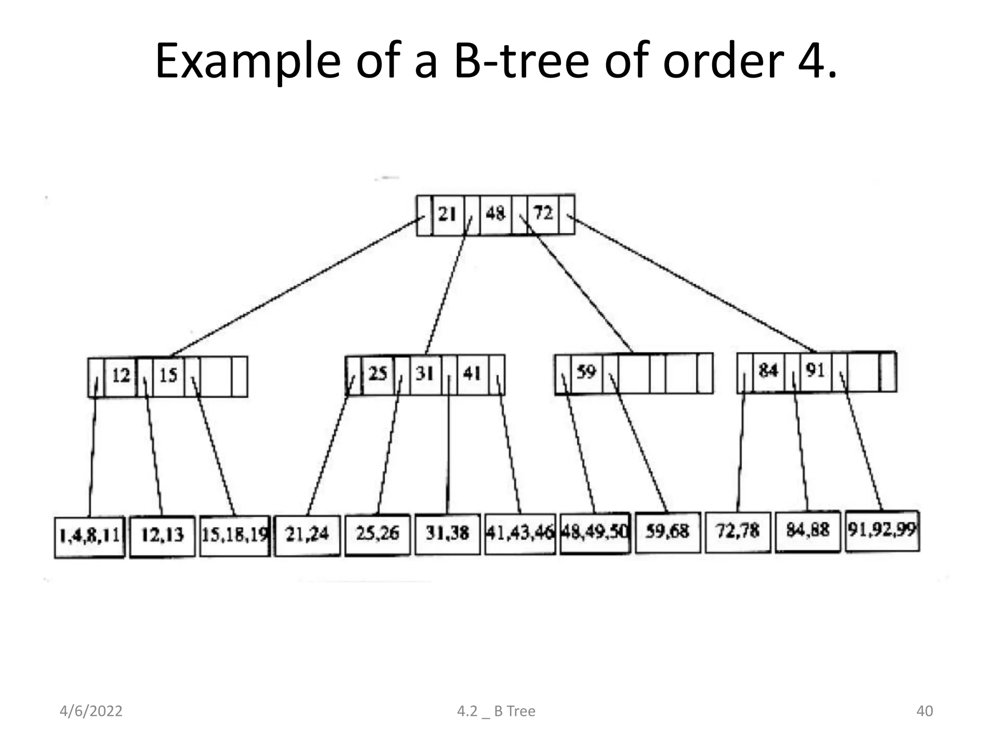
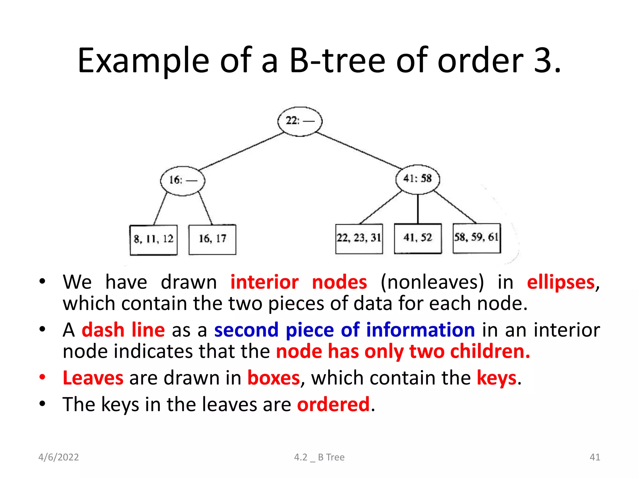
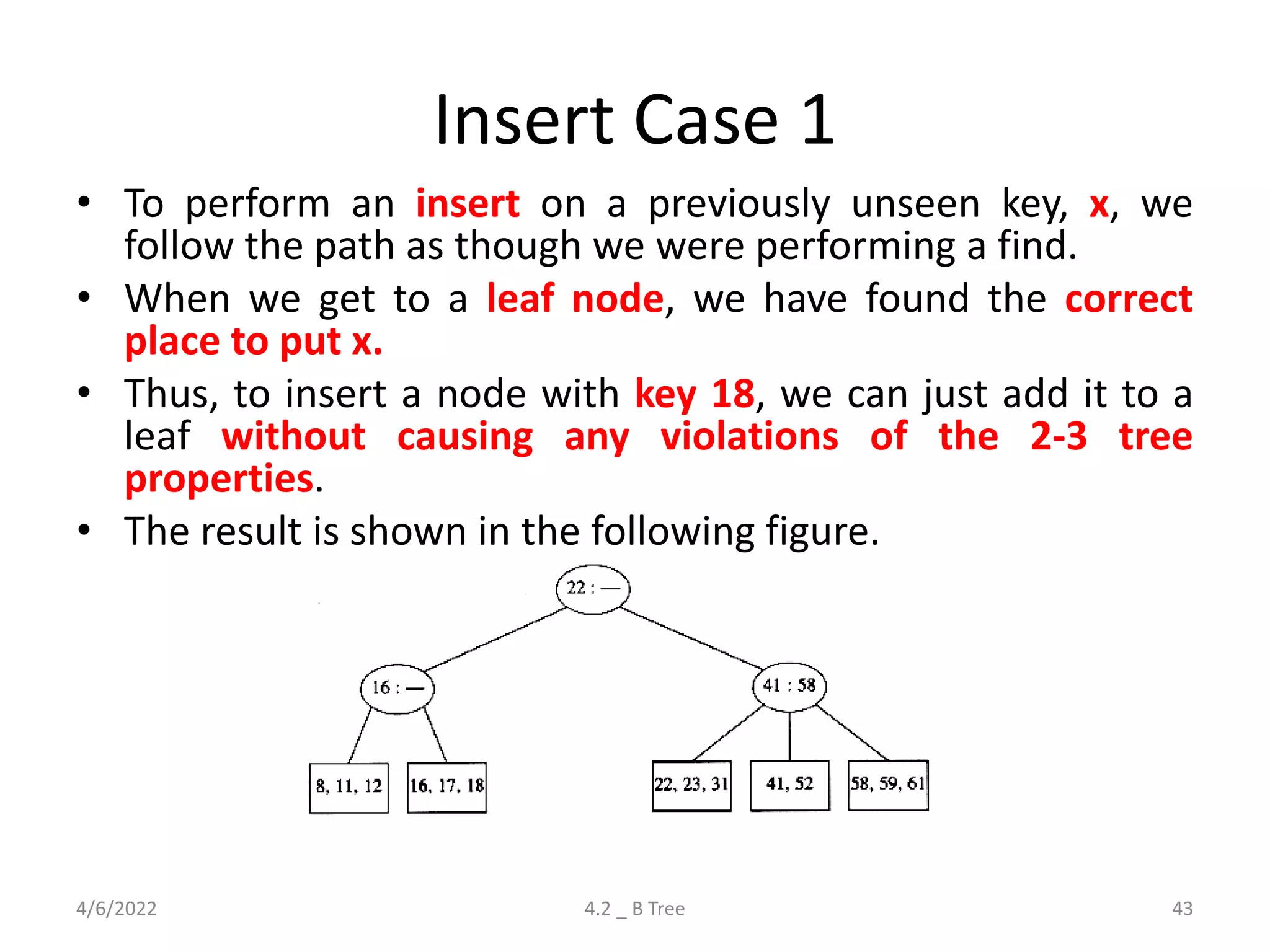
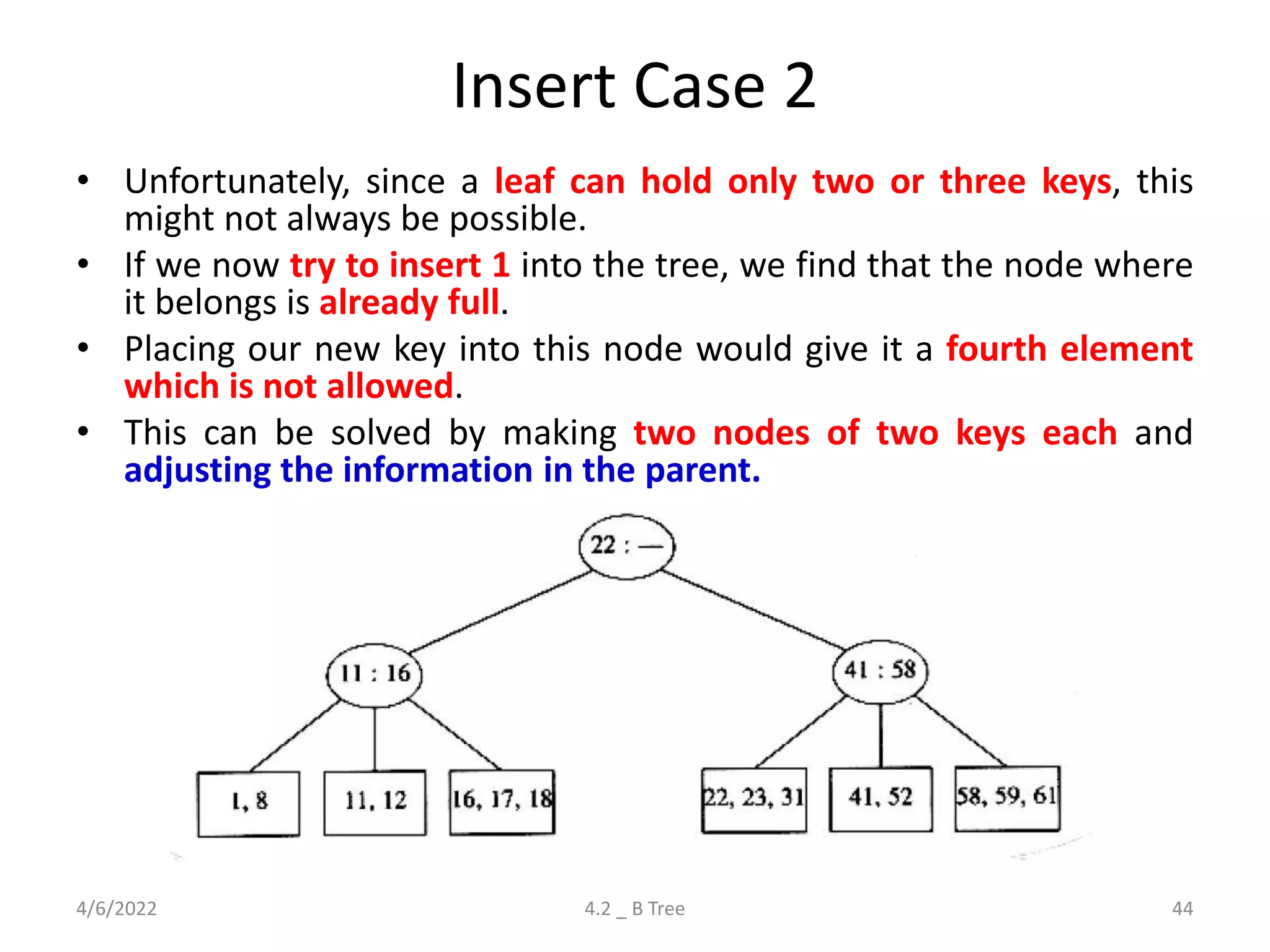
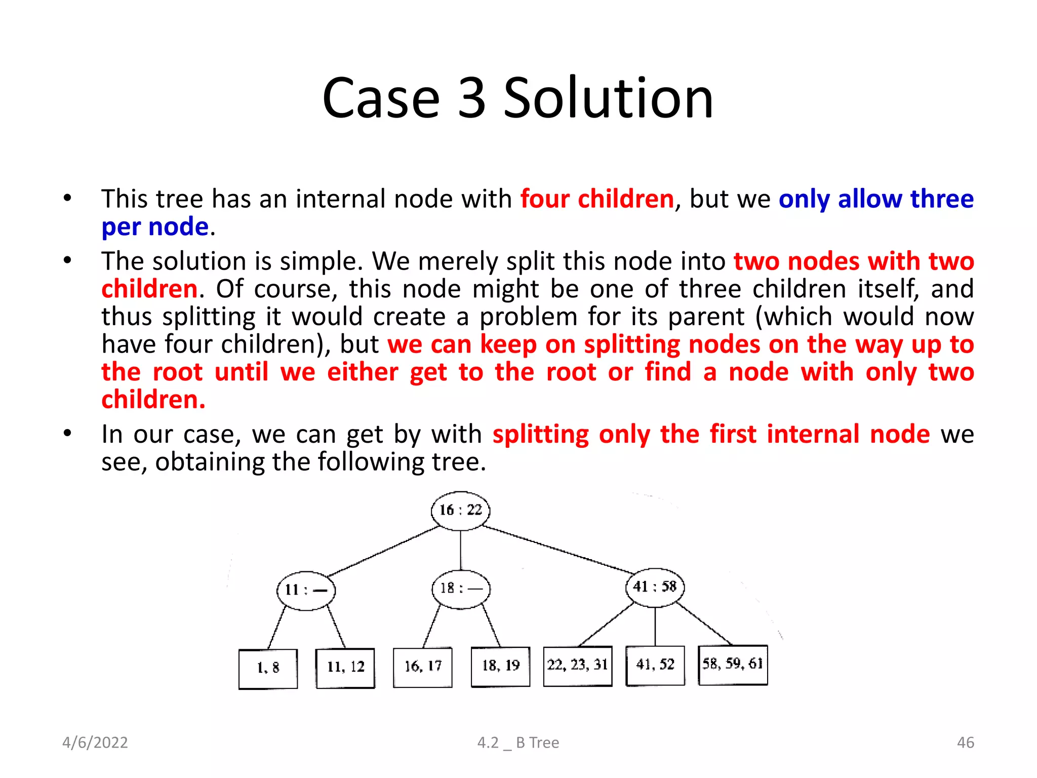
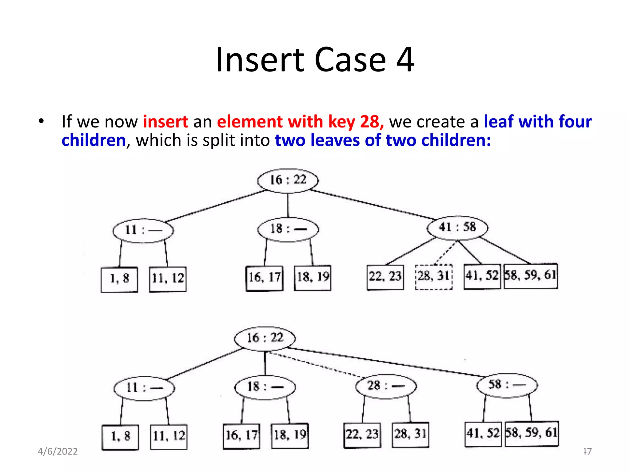
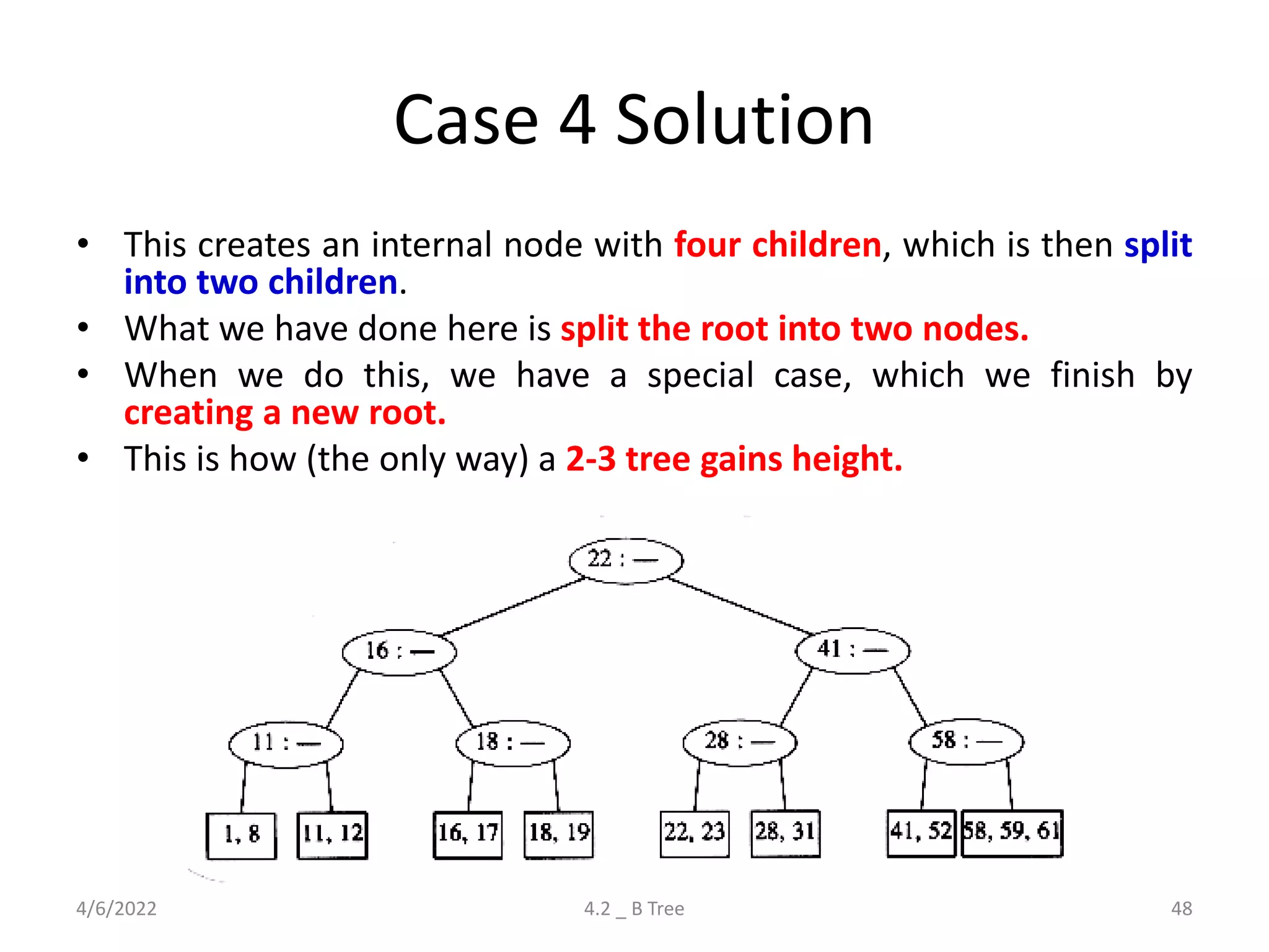
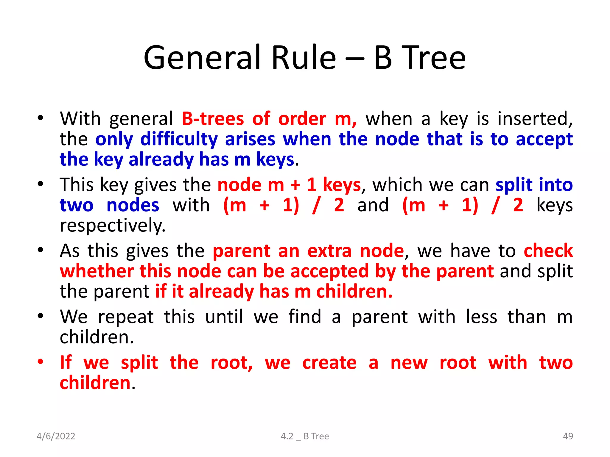
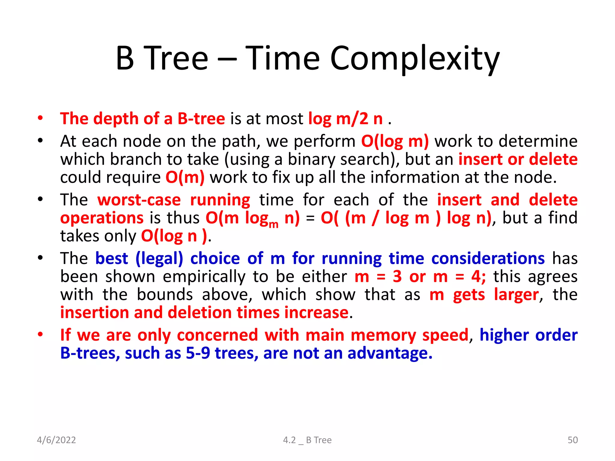
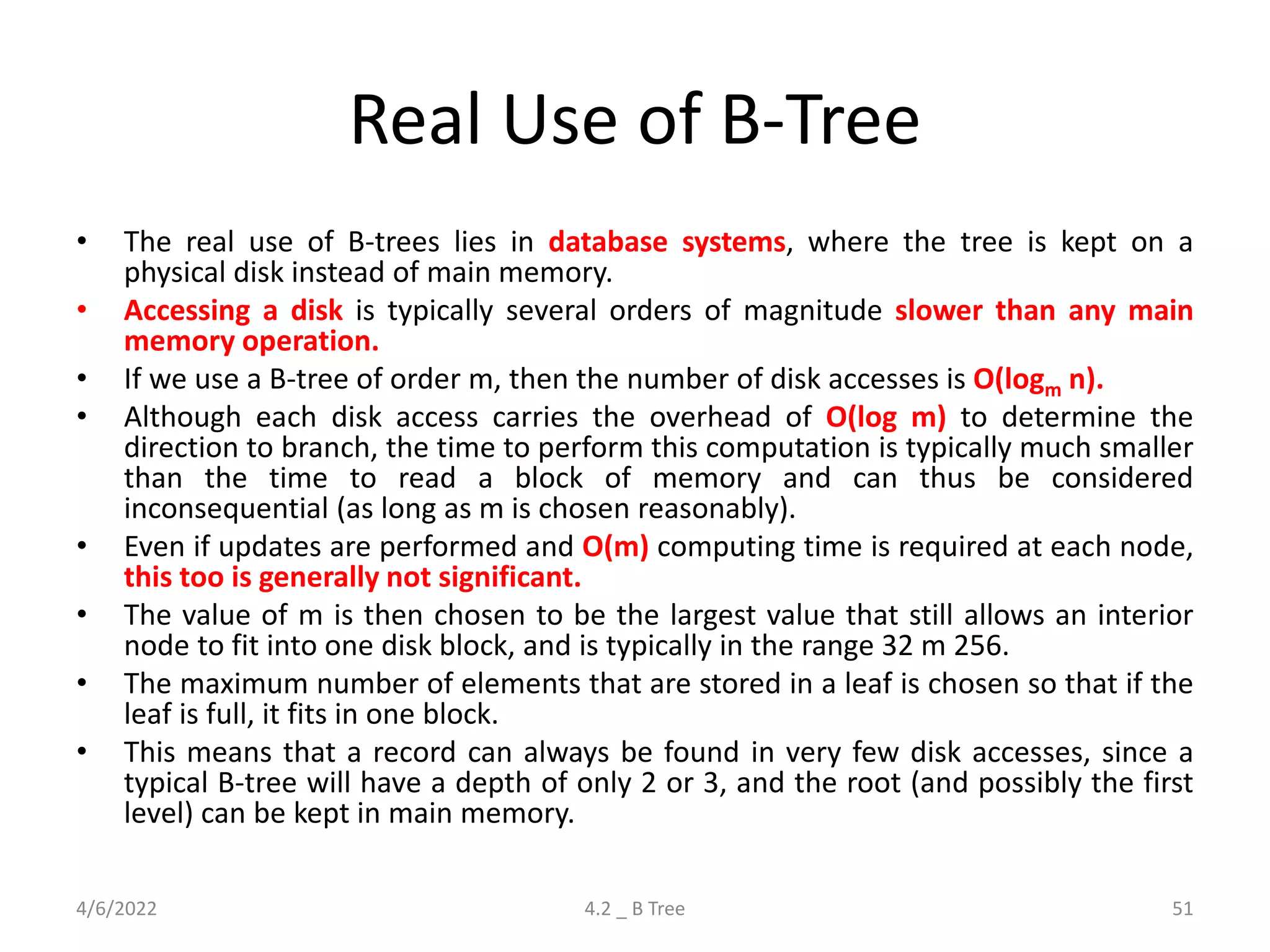
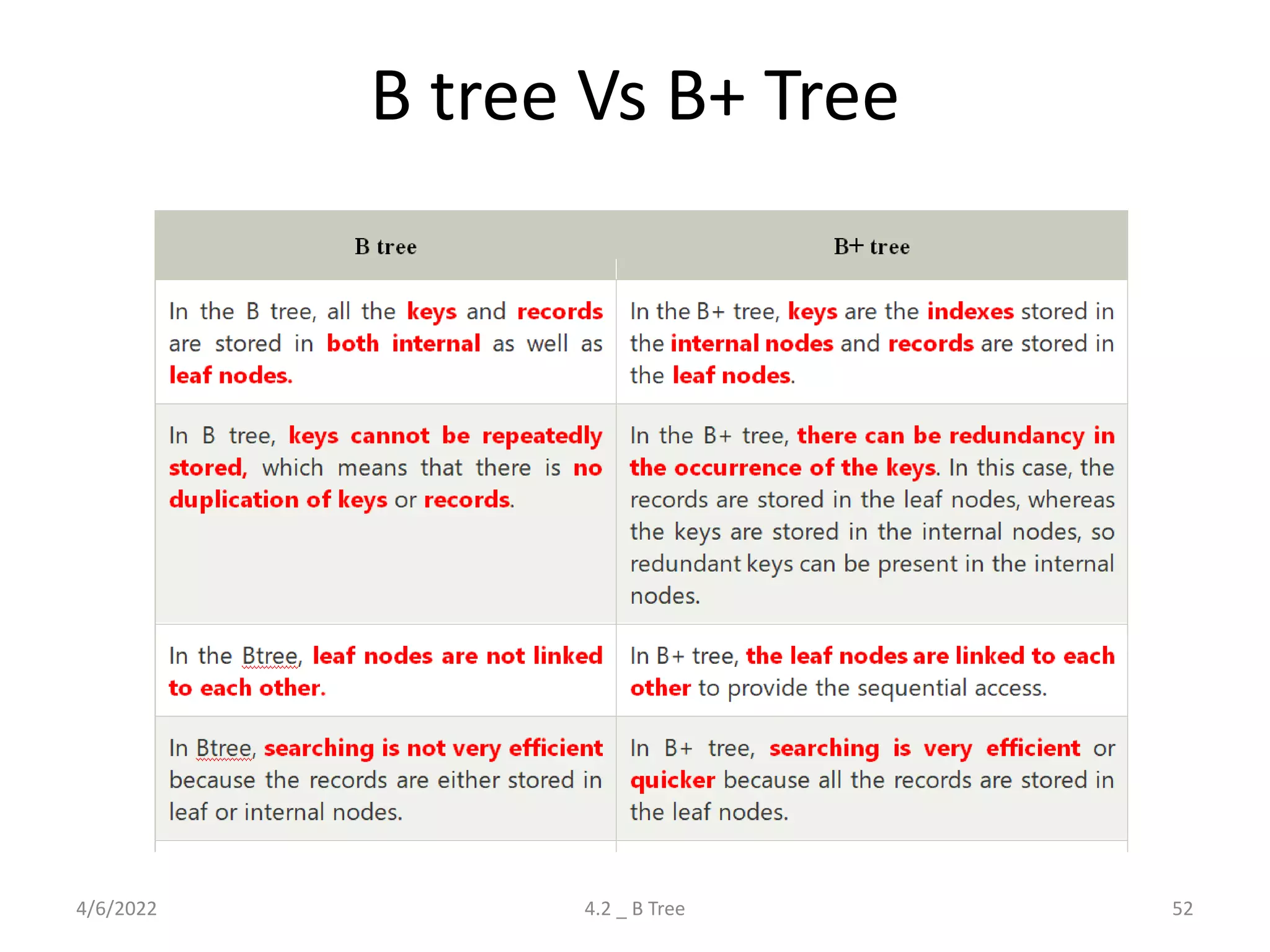
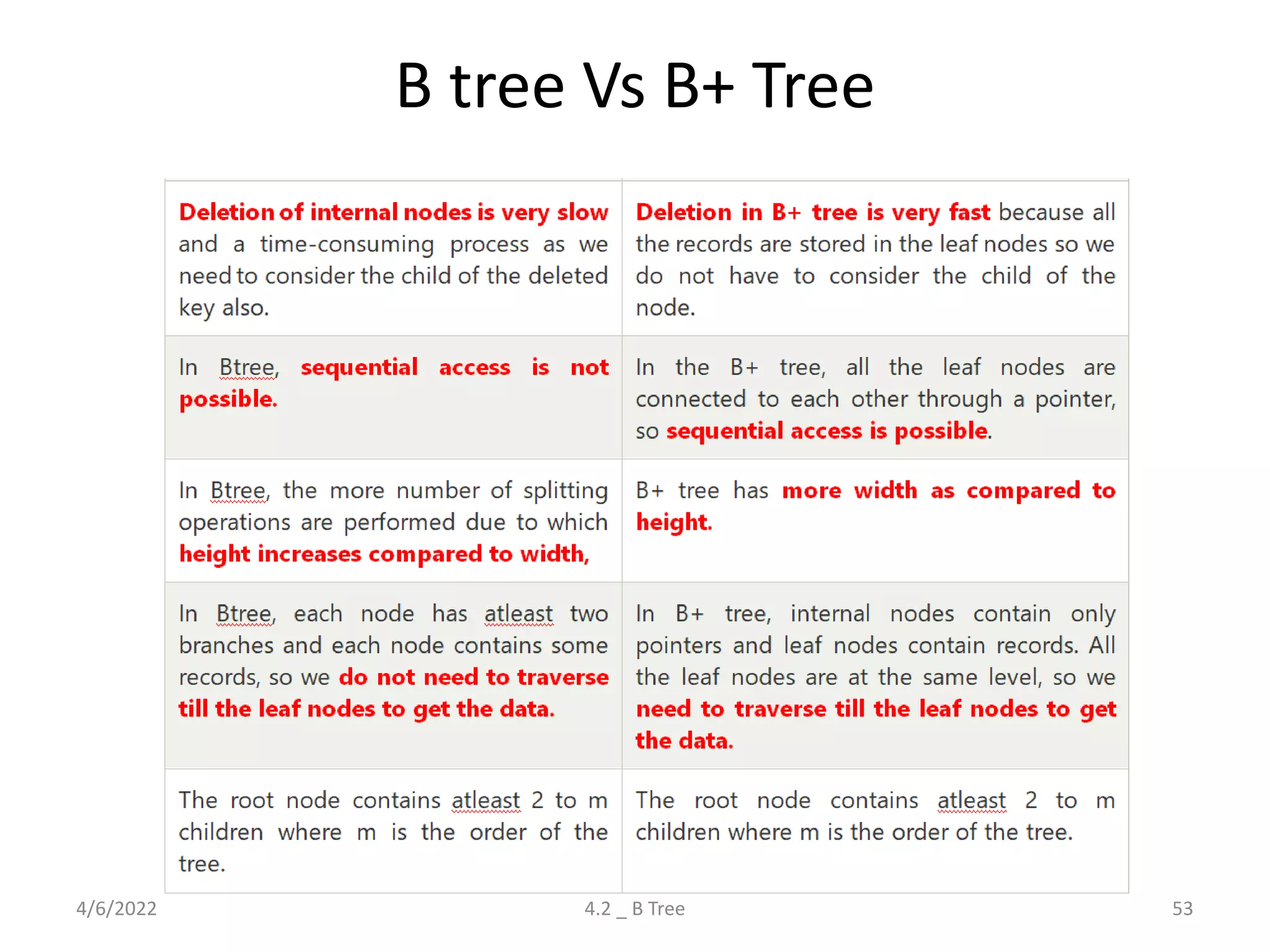
Detailed explanation of B Trees' structure, properties, operations, and comparison with B+ Trees.
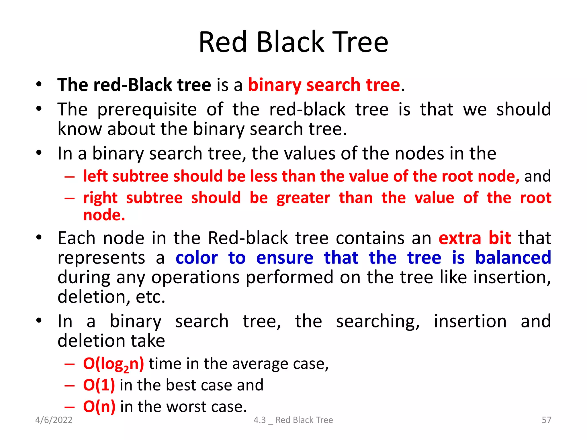
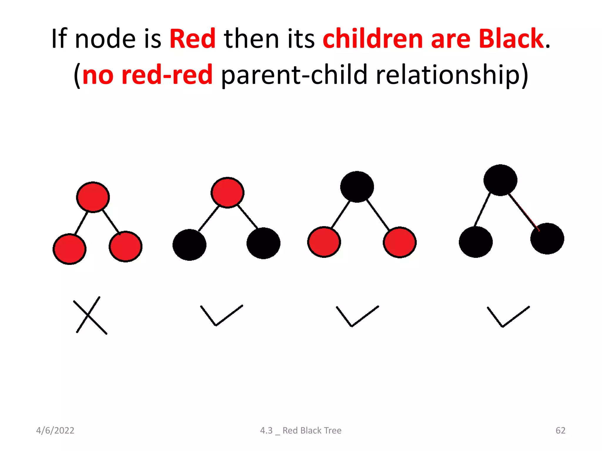
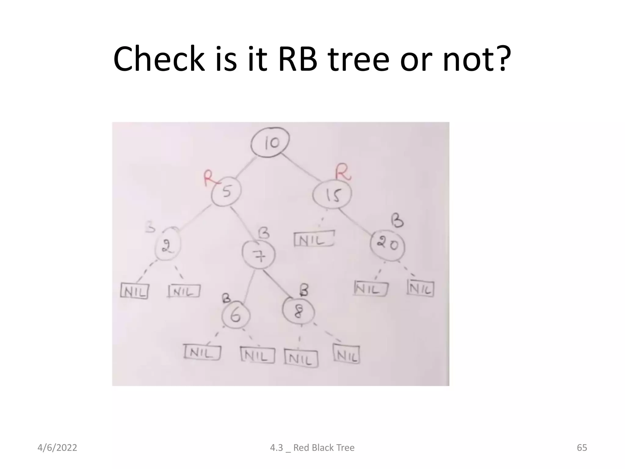
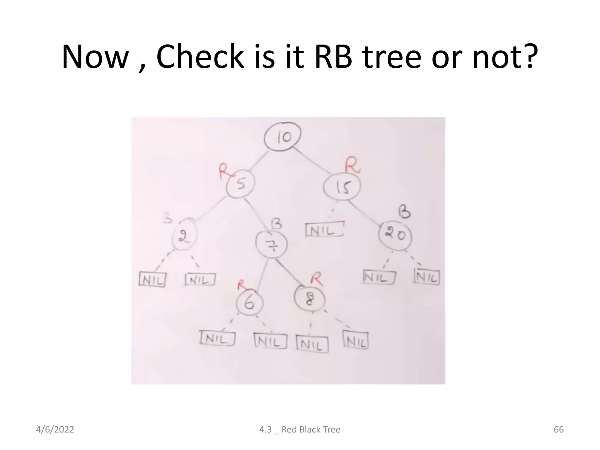
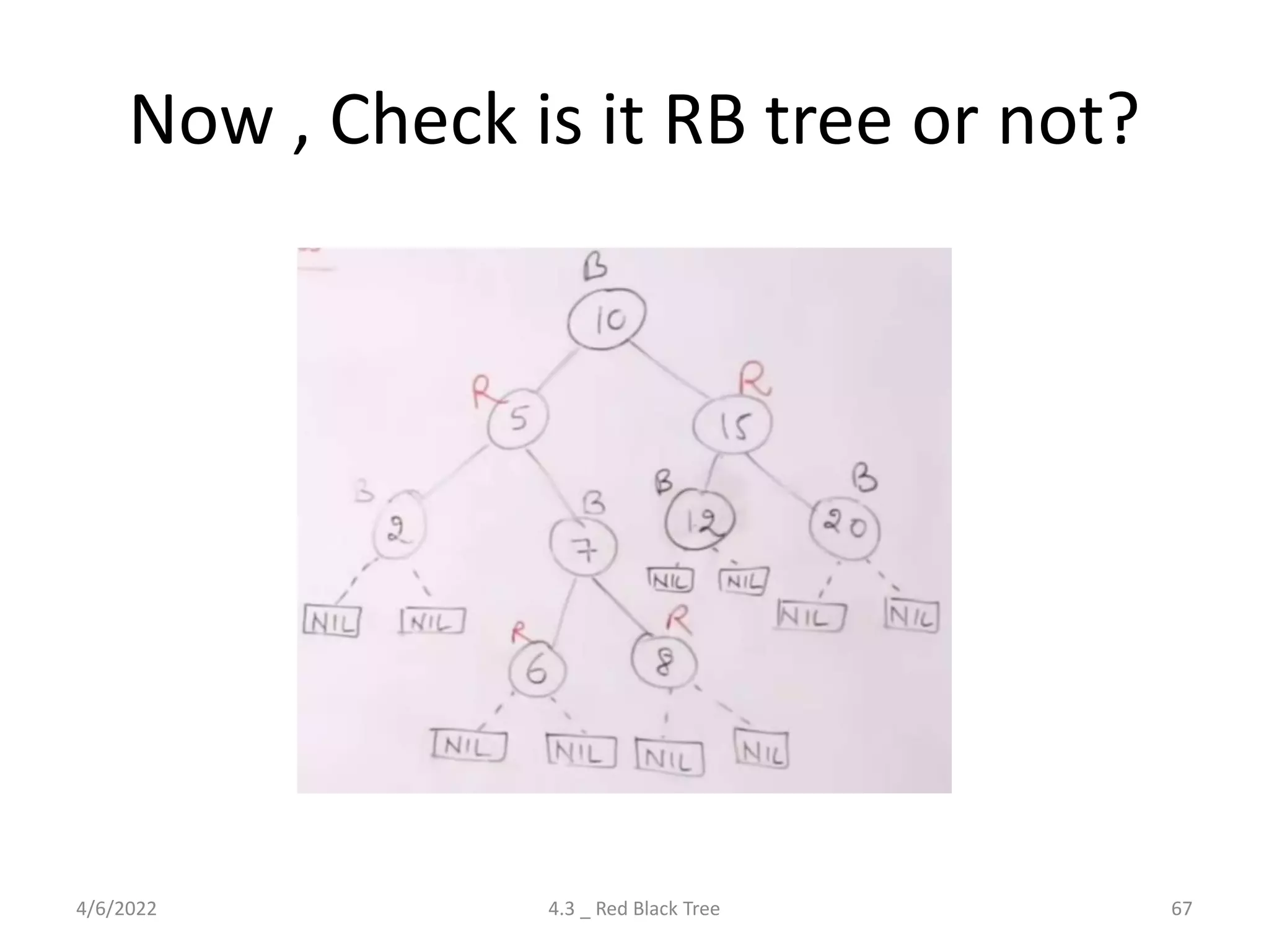
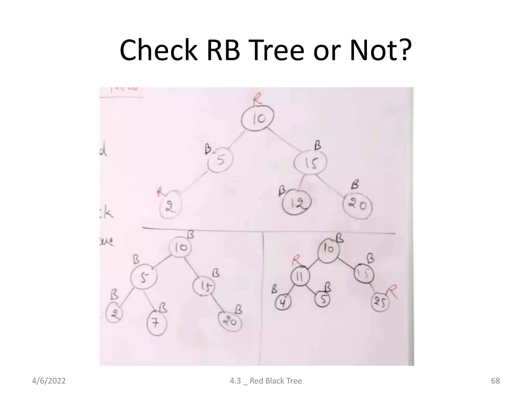
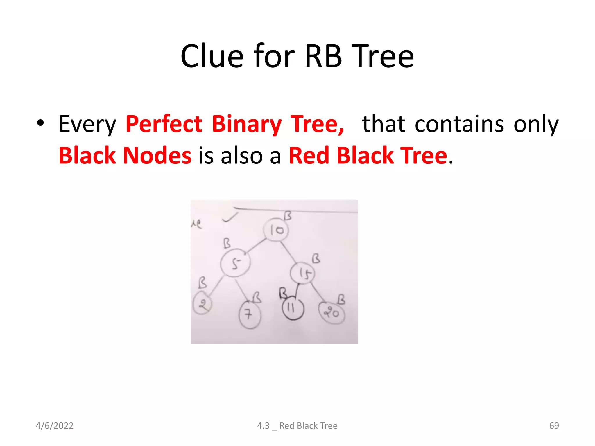
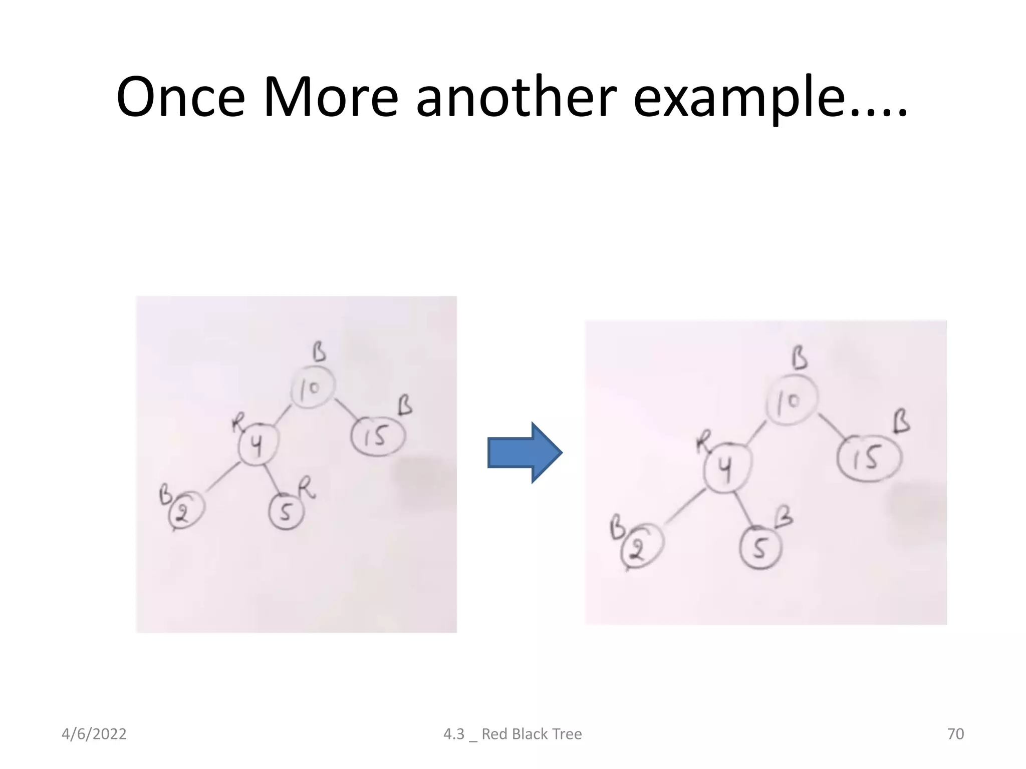
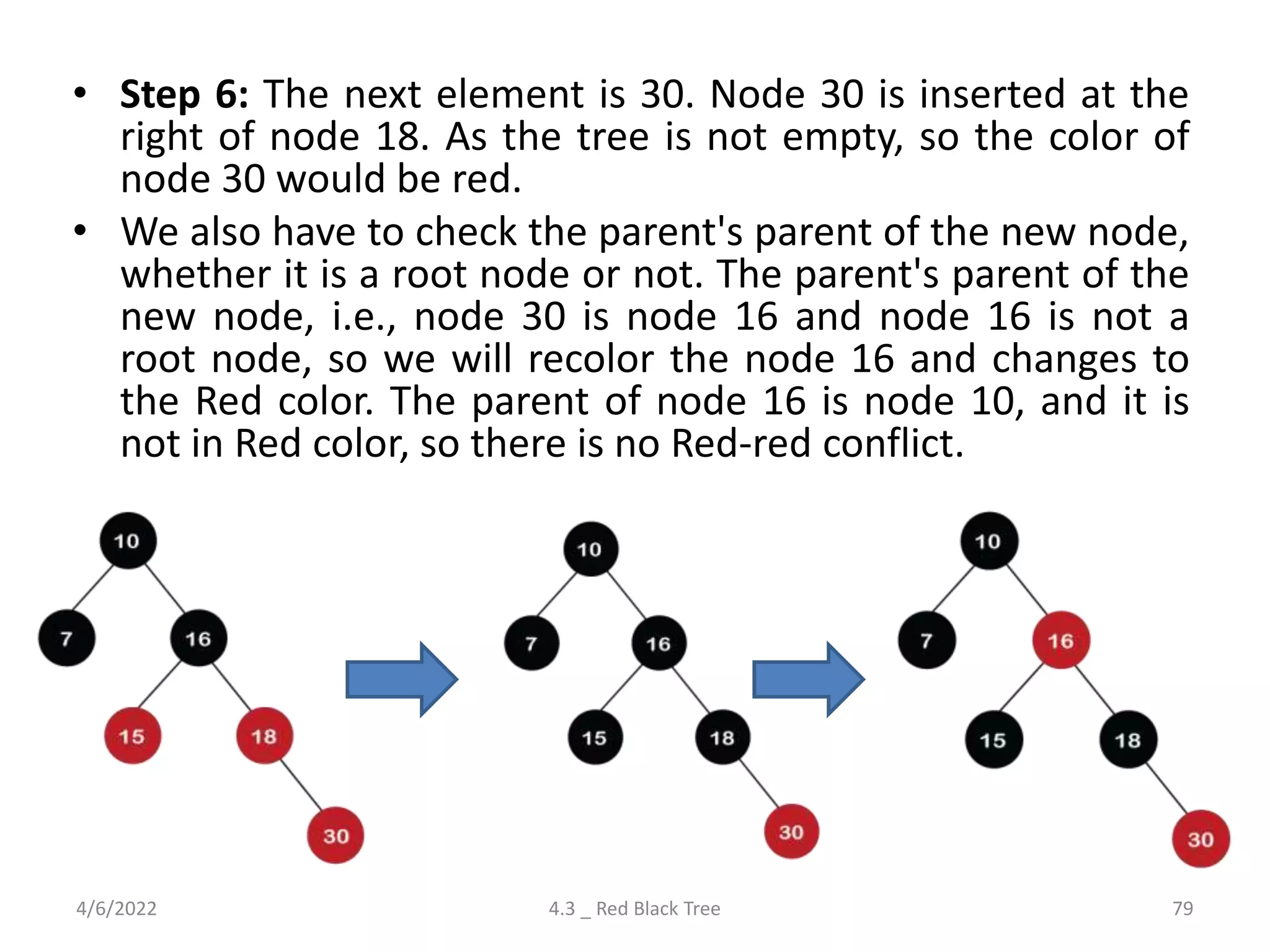
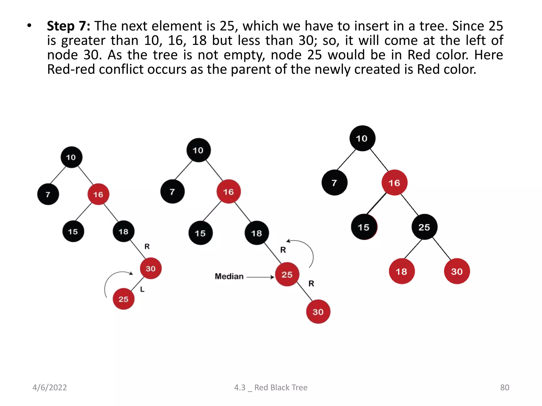
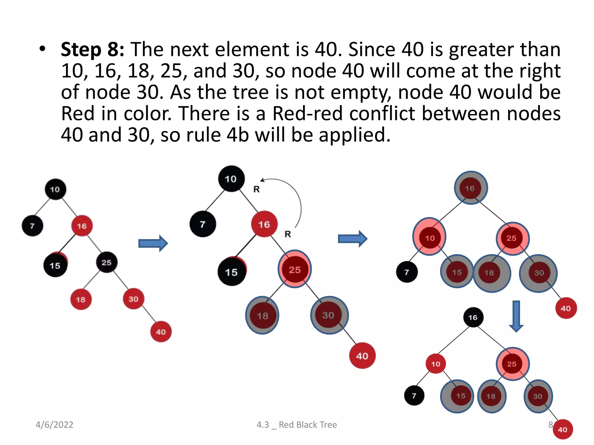
Comprehensive look at Red-Black Trees, including properties, insertion, deletion rules, and differences from AVL trees.
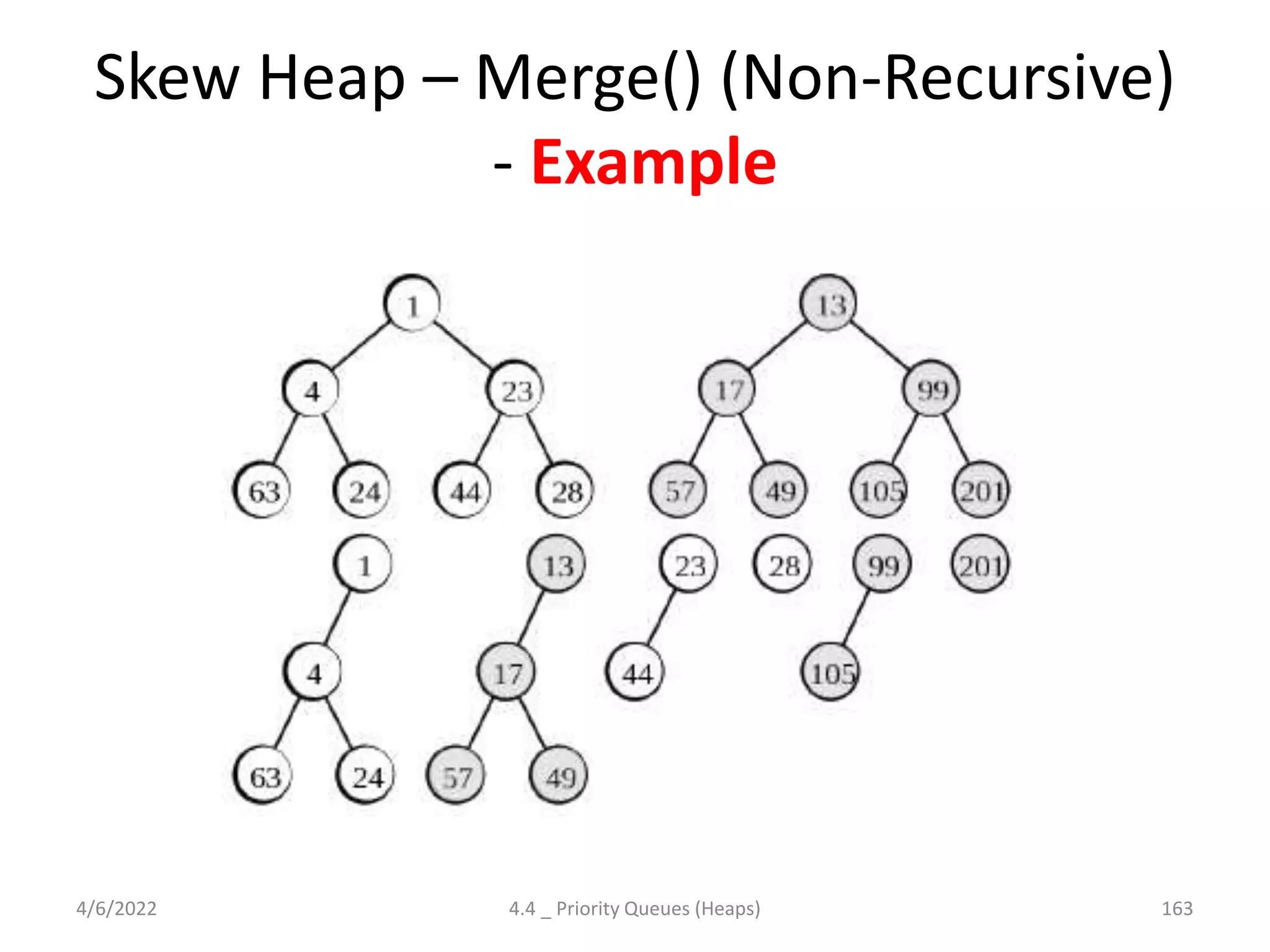
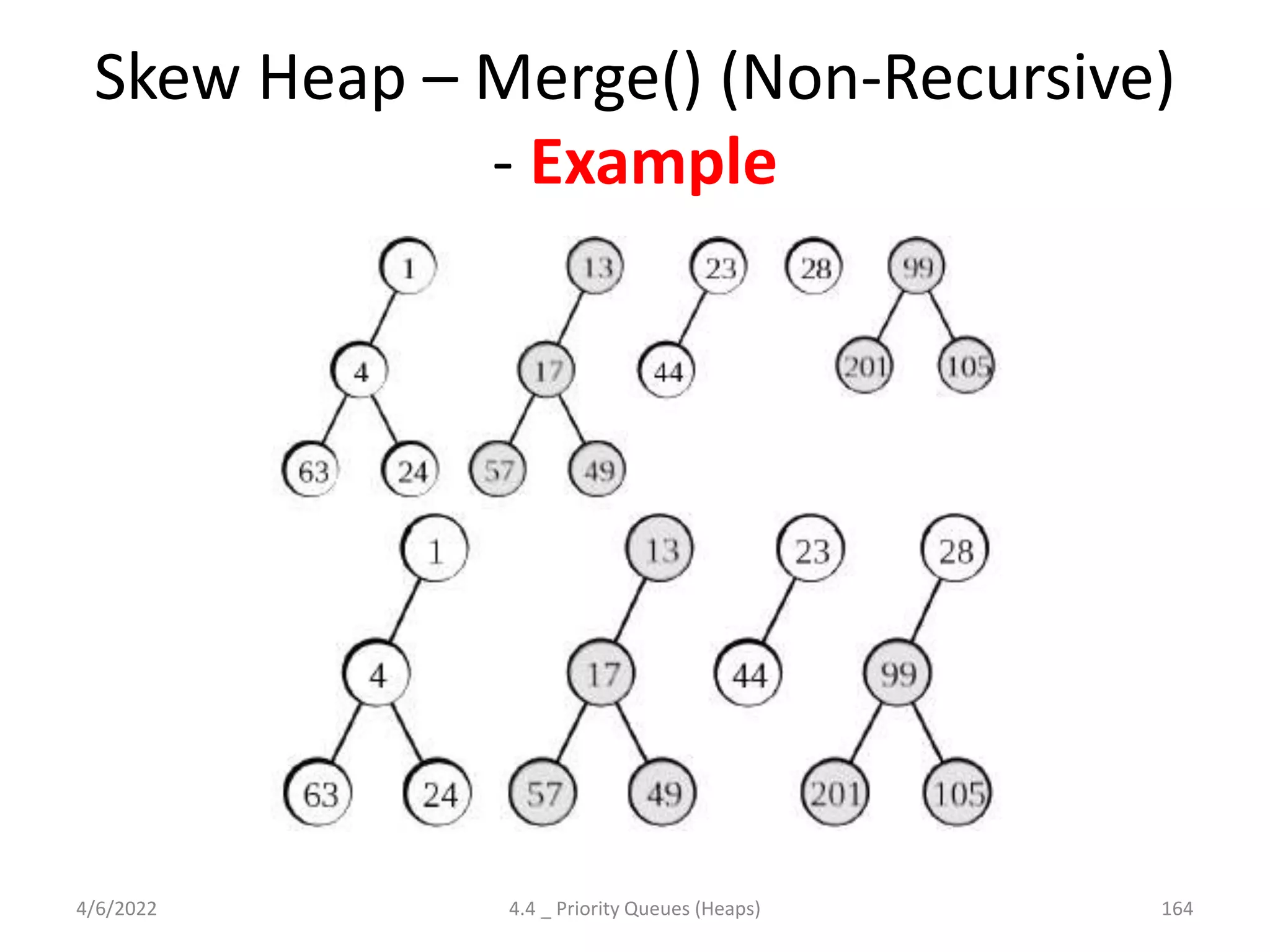
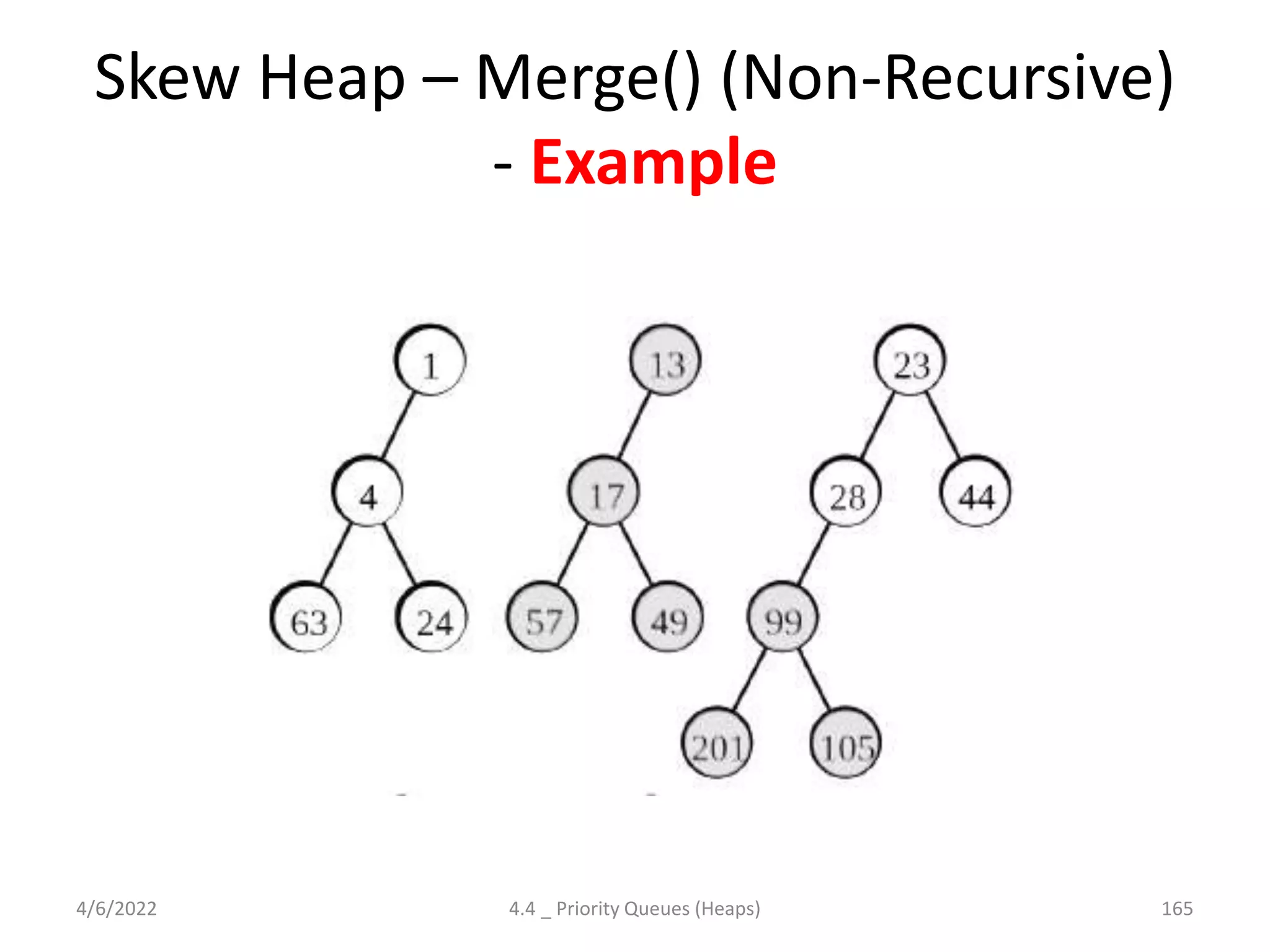
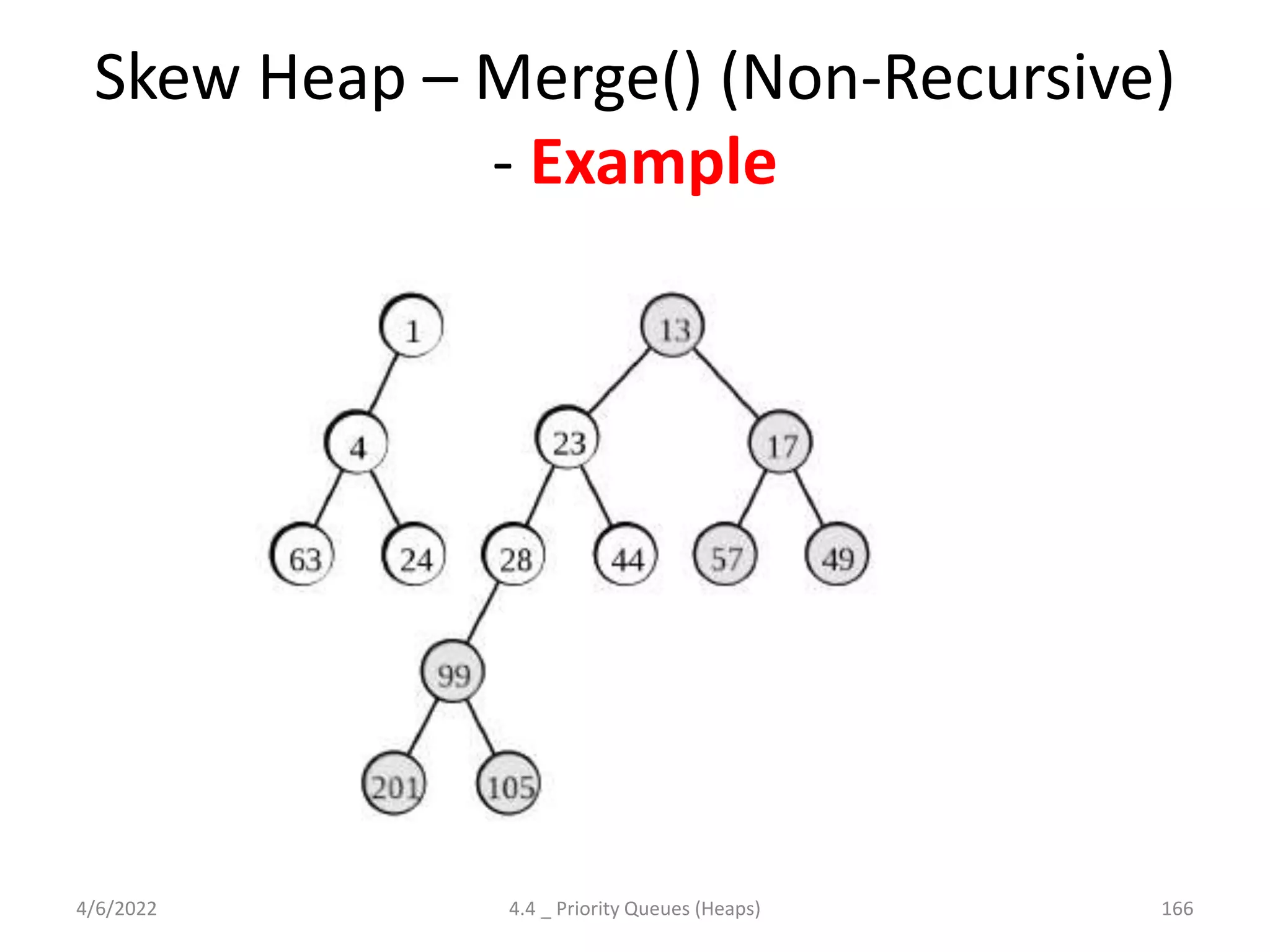
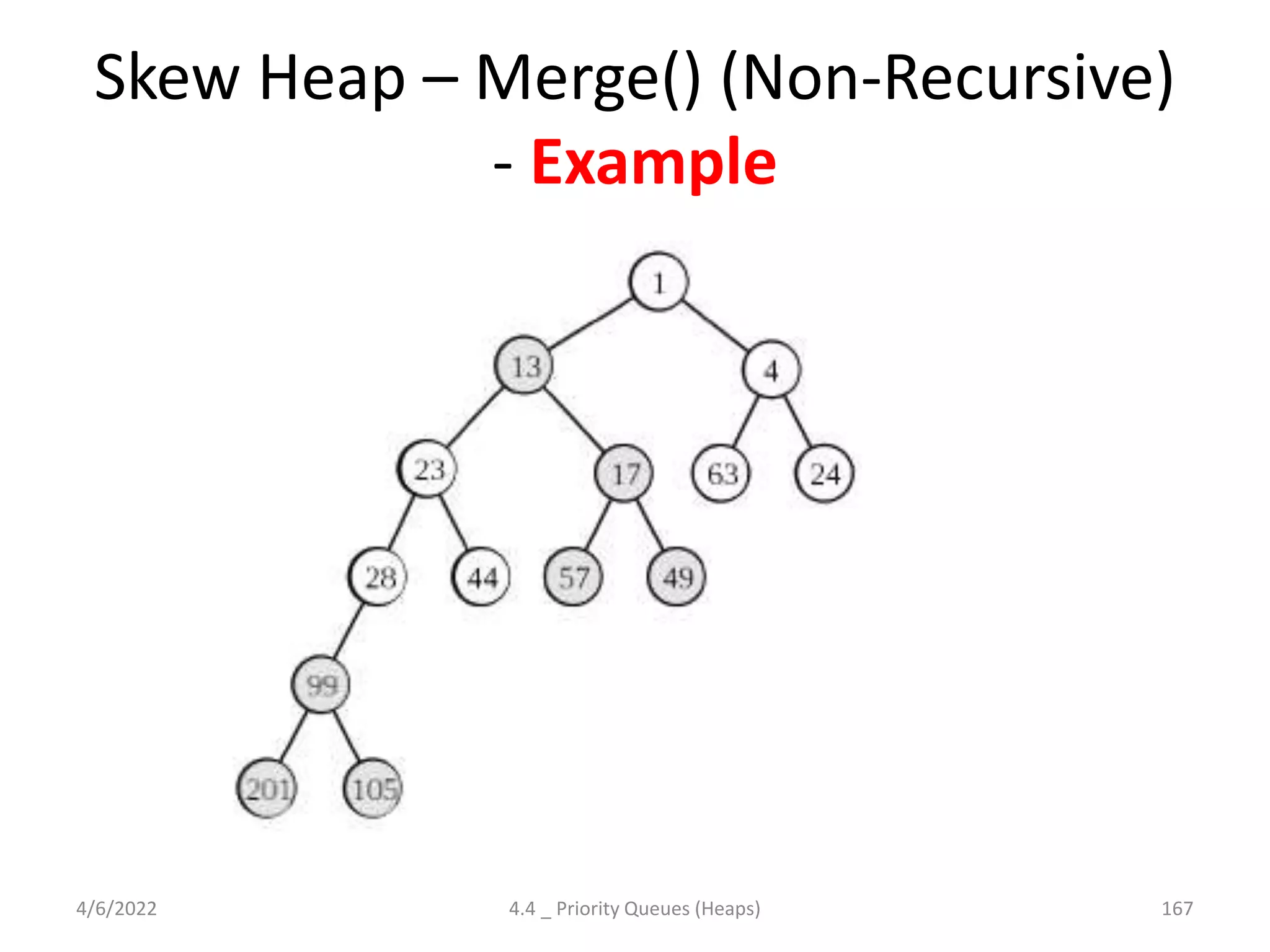
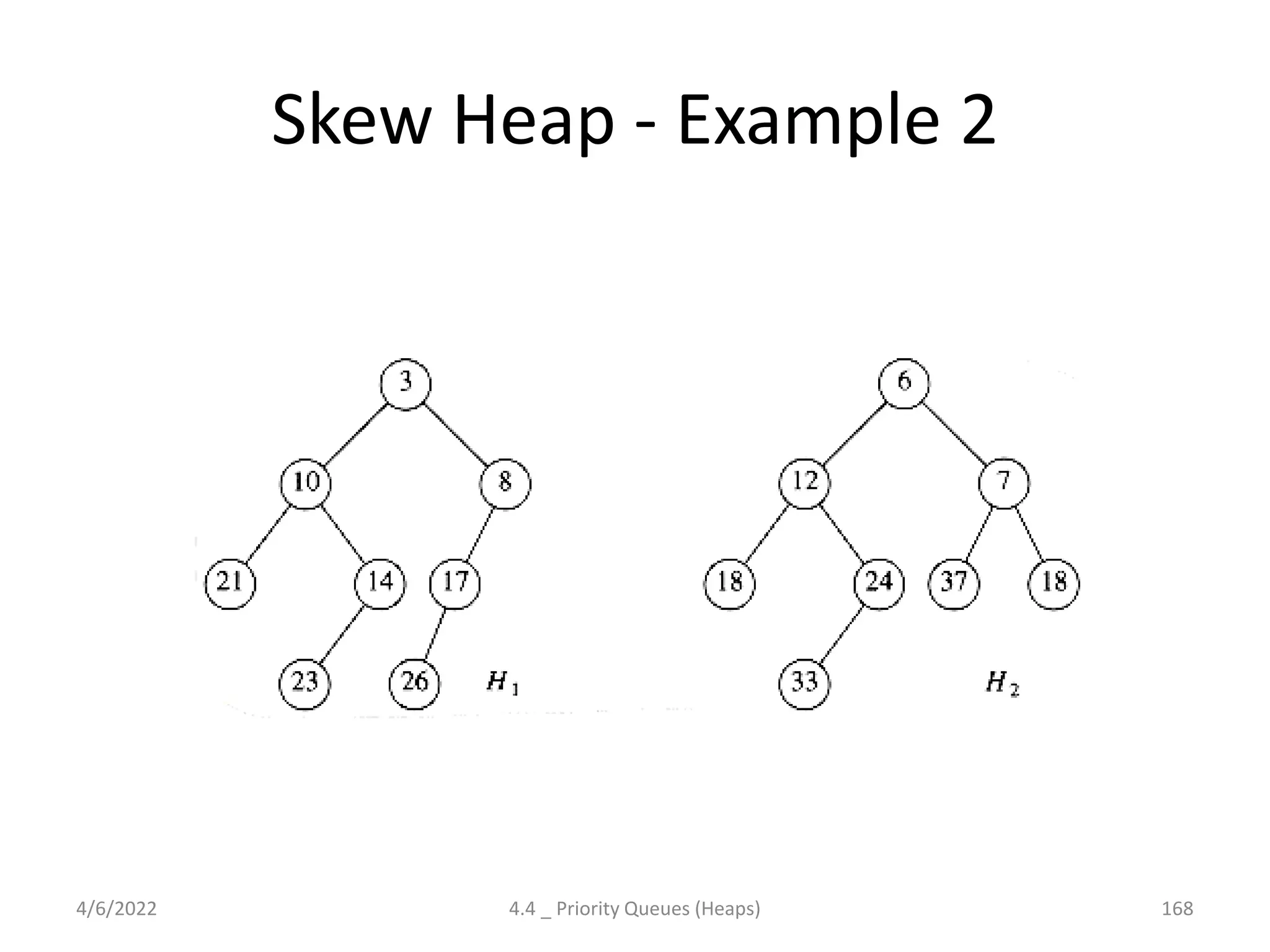
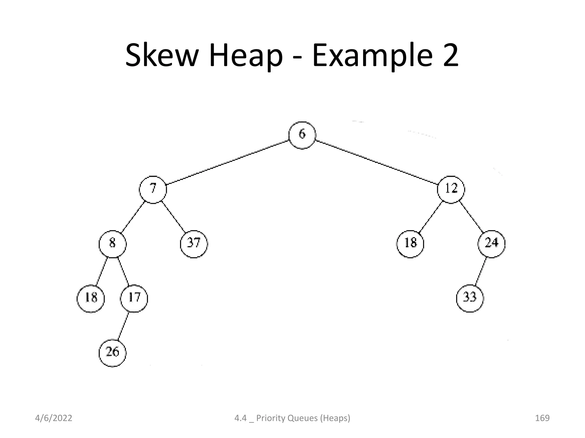
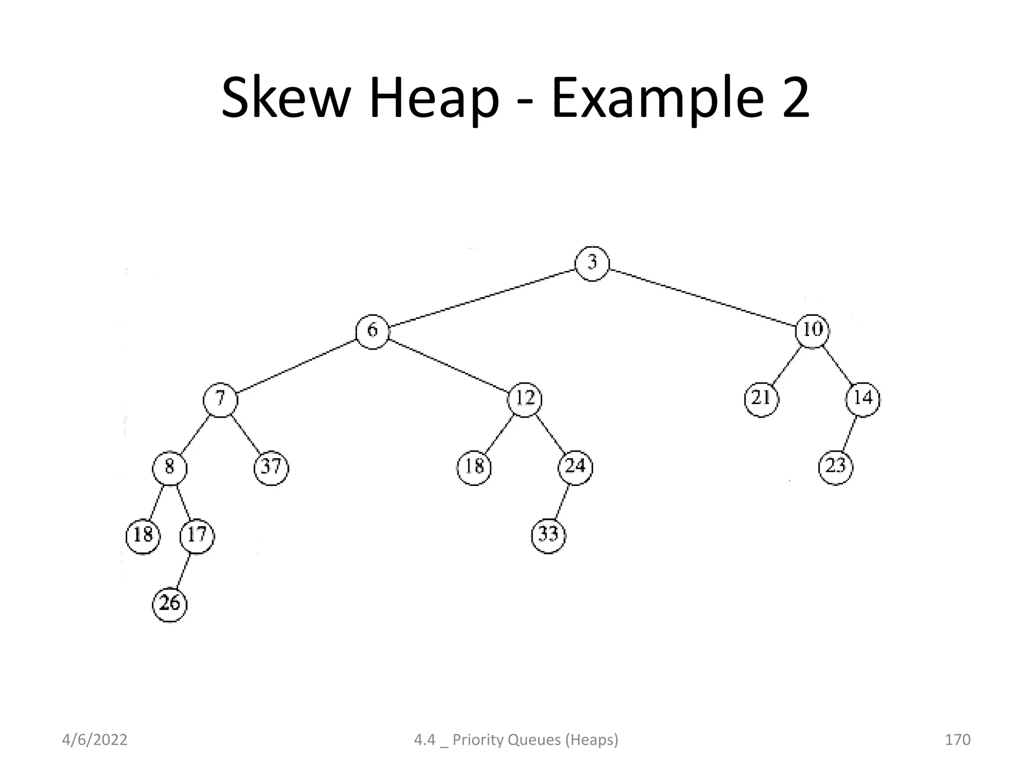
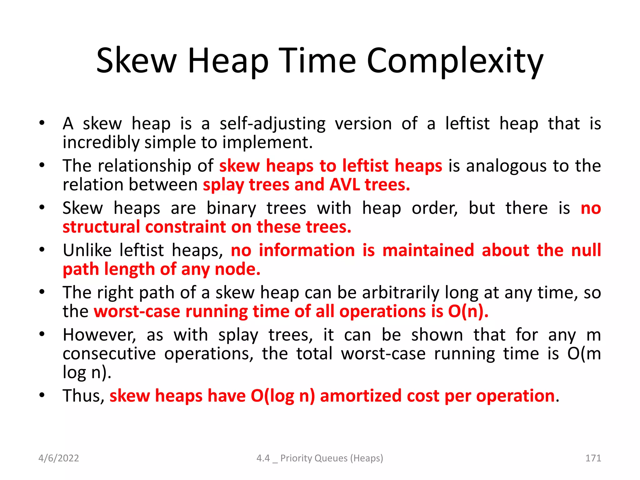
Discusses Priority Queues' necessity, implementations (Binary Heap, Leftist Heap, Skew Heap), time complexities, and applications.


![Depth first search [dfs]](https://cdn.slidesharecdn.com/ss_thumbnails/depthfirstsearchdfs-190926145304-thumbnail.jpg?width=640&height=640&fit=bounds)


![[PPT] _ Unit 2 _ 9.0 _ Domain Specific IoT _Home Automation.pdf](https://cdn.slidesharecdn.com/ss_thumbnails/pptunit29-220516115946-098632b6-thumbnail.jpg?width=640&height=640&fit=bounds)

![[PPT] _ UNIT 1 _ COMPLETE.pptx](https://cdn.slidesharecdn.com/ss_thumbnails/pptunit1complete-220516121012-45cab1a3-thumbnail.jpg?width=640&height=640&fit=bounds)
![[PPT] _ Unit 5 _ Evolve.pptx](https://cdn.slidesharecdn.com/ss_thumbnails/pptunit5evolve-220707120639-5c6df843-thumbnail.jpg?width=640&height=640&fit=bounds)


![[PPT] _ Unit 3 _ Experiment.pptx](https://cdn.slidesharecdn.com/ss_thumbnails/pptunit3experiment-220707114954-1996fe08-thumbnail.jpg?width=640&height=640&fit=bounds)
![[PPT] _ Unit 4 _ Engage.pptx](https://cdn.slidesharecdn.com/ss_thumbnails/pptunit4engage-220707115545-9dce3530-thumbnail.jpg?width=640&height=640&fit=bounds)


