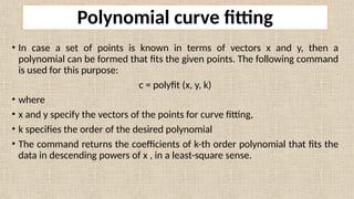
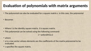
The document provides a comprehensive guide on polynomials in MATLAB, covering their definitions, evaluation, roots, addition, subtraction, multiplication, division, differentiation, integration, and curve fitting. It explains the use of various functions such as 'polyval', 'roots', 'polyder', 'polyint', and 'polyfit' with examples. Additionally, it demonstrates evaluating polynomials using matrix arguments through the function 'polyvalm'.

1. MATLAB
Module 03 Part 01
Prepared by: Amit Uniyal
THDC IHET
FOR LAB - Programming Practices

2. Polynomials
• A polynomials is an expression in which a finite number of constants and
variables are combined using addition, subtraction, multiplication and non-
negative whole number exponents (raise to power).
• Consider a polynomial
This can be entered as a row vector p(s) follows:
p = [1, 3, -15, -2, 9]
Elements of vector p are five in number with the last element being the
constant term. The order of the polynomial represented by vector p is four.

3. Polynomial Evaluation
• A polynomial can be evaluated for a given value of variable. By using the function
“polyval”. The general form of the function “polyval” is as follows:
polyval (c, s)
Where
c is a vector whose elements are the coefficients of a polynomial in descending order of
powers of variables s, and s is the value at which the polynomial is to be evaluated.
Exp - at s = 1
y = [2, 3, 4];
s = 1;
value = polyval (y, s)
value = 9

4. Roots of a Polynomial
• The roots of a polynomial can be found using the MATLAB function:
roots (p)
or , r = roots (p)
where “p” is a row vector containing the coefficients of a polynomial. It returns
a column vector “r” whose elements are the roots of the polynomial.
Exp-
p = [1 3 2];
r = roots(p);
r = -2, -1

5. Polynomial Addition and Subtraction
• Two polynomial can be added by using the arithmetic operator “+”, i.e. if
two polynomials x and y are to be added, the following command can be
used:
z = x + y
• Similarly, subtraction is done by using operator “-” and the syntax is given as
follows:
z = x - y

6. Polynomial Multiplication & Division
• Multiplication
z = conv(x, y)
x and y are the vectors of coefficients of polynomials to be multiplied, and z
contains the coefficients of the resultant polynomial.
• Division
[z, r] = deconv(x, y)
x is the dividend vector,
y is the divisor vector,
z specifies the vector of quotients obtained, and
r specifies the vector of remainders obtained.

7. Polynomial Differentiation
• The function polyder is used to compute the derivative of a polynomial. The
general form of this function is
dydx = polyder(y)
where
y represents the vector of the coefficients of the polynomials whose derivative
is to be obtained, and
dydx represents the vector of the coefficients of the derivative obtained.
Ex-
Solution:- y = [1 4 8 1 3];
dydx = polyder(y)
dxdy = 4 12 16 1 0

8. Polynomial integration
• The function polyint is used to compute the integration of a polynomial. The general
form of this function is:
polyint(y, k) or
x= polyint(y, k)
• where, y represents the vector of the coefficients of the polynomials whose
integration is to be obtained, and k is the scalar constant of integration and x
contains the result.
• Exp – Integrate the polynomial , take constant of integration as 3.
Sol.
y = [4 12 16 1]; x = polyint(y, 3)
x = 1 4 8 1 3
• The resultant vector gives the coefficients of the polynomial representing the
integral of polynomial y.

9. Polynomial curve fitting
• In case a set of points is known in terms of vectors x and y, then a
polynomial can be formed that fits the given points. The following command
is used for this purpose:
c = polyfit (x, y, k)
• where
• x and y specify the vectors of the points for curve fitting,
• k specifies the order of the desired polynomial
• The command returns the coefficients of k-th order polynomial that fits the
data in descending powers of x , in a least-square sense.

10. x 0 1 2 4
y 1 6 20 100
Exp- Find a polynomial of degree 2 to fit the following data:
Solution:-
x and y are represented by the following row vectors:
x = [0 1 2 4];
y = [1 6 20 100];
the command
c = polyfit(x, y, 2)
c = 7.3409 -4.8409 1.6818
hence, the polynomial is 7.3409x2 - 4.8409x + 1.6818

11. Evaluation of polynomials with matrix arguments
• The polynomial can also be evaluated for a square matrix s. in this case, the polynomial
• Becomes
• Where I is the identity square matrix, S is square matrix.
• This polynomial can be solved using the following command:
z = polyvalm(a,s)
• where
• a is a row vector whose elements are the coefficients of the matrix polynomial to be
evaluated
• s specifies the square matrix.

12. • Exp – Evaluate the matrix polynomial , given that the square matrix X is.
X = [2 3; 4 5]
• Solution
The commands used are:
A = [1 1 2];
X = {2 3; 4 5];
Z = polyvalm(A, X)
• Result – Z = 20 24; 32 44