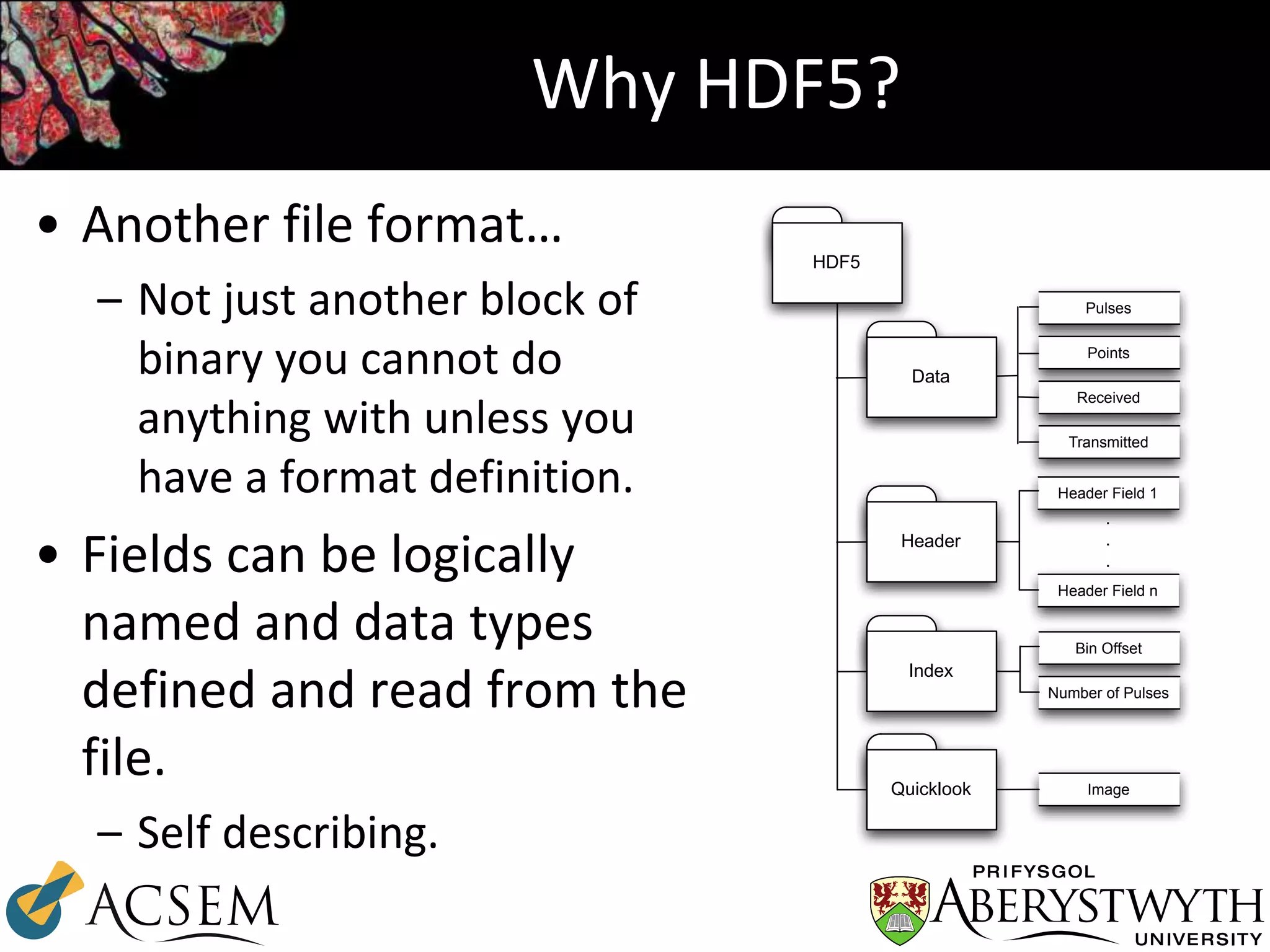
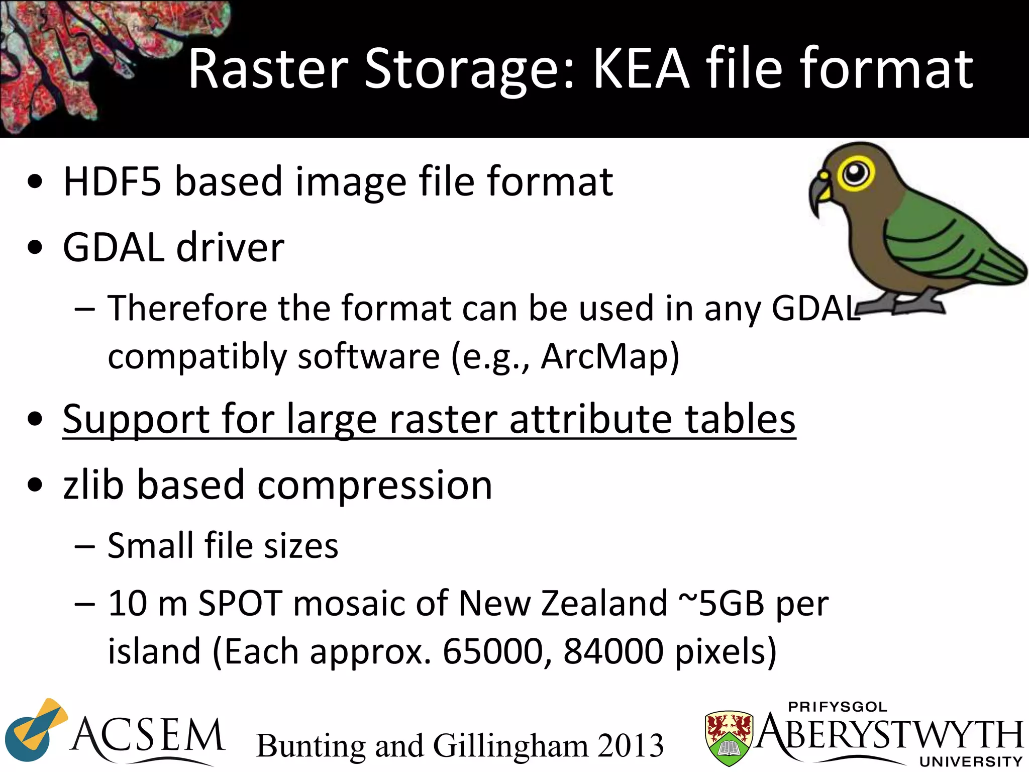
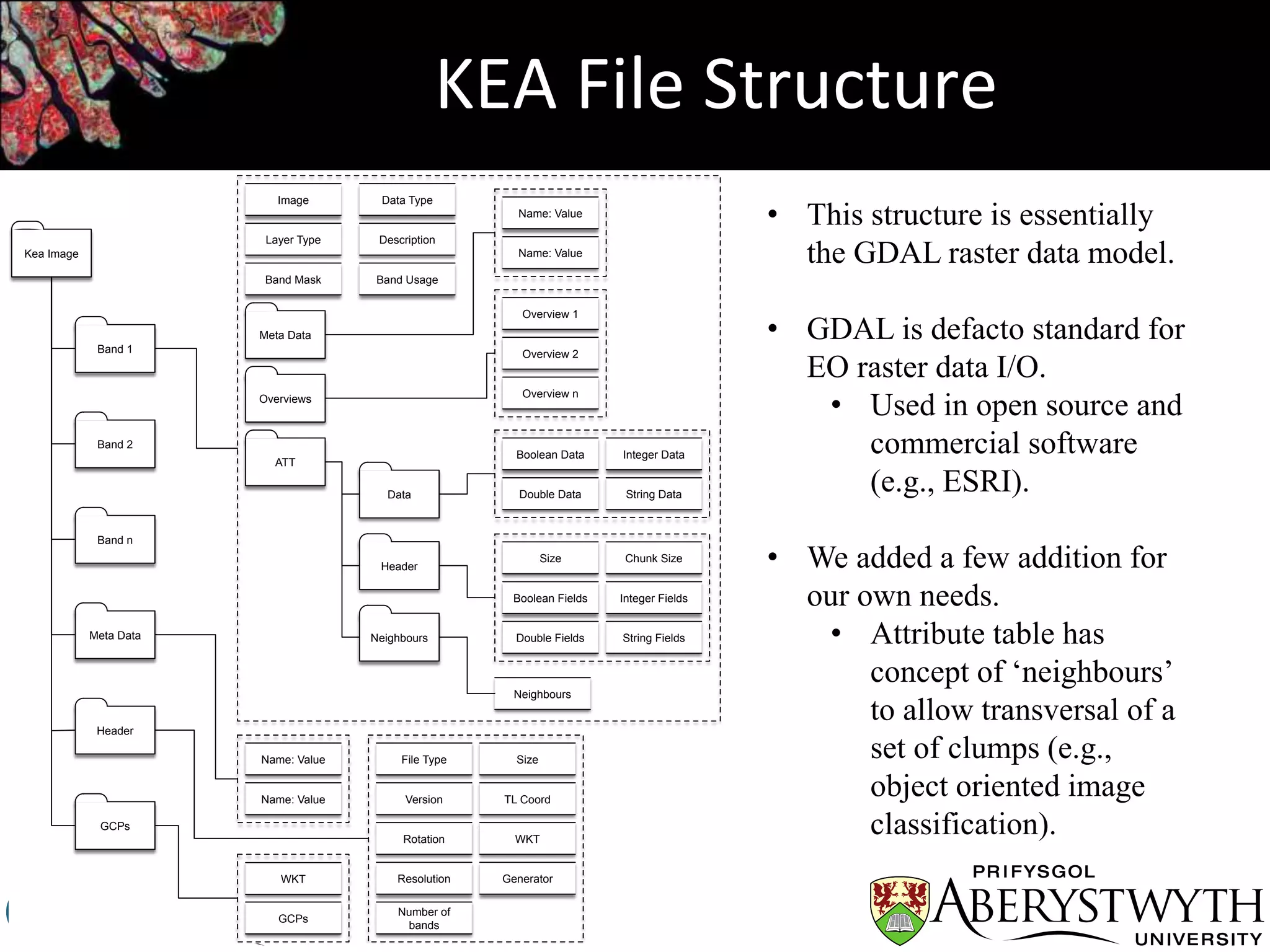
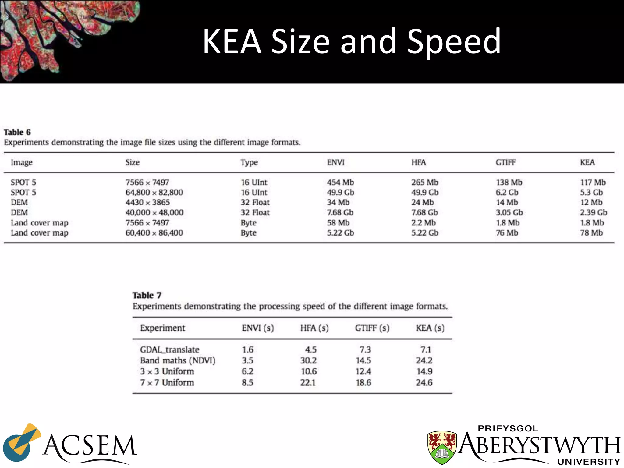
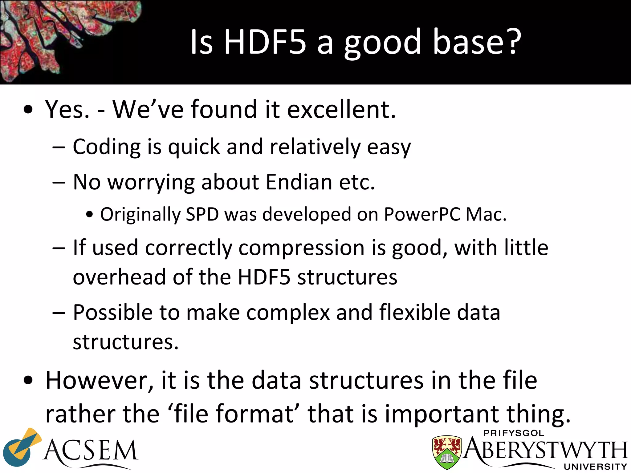
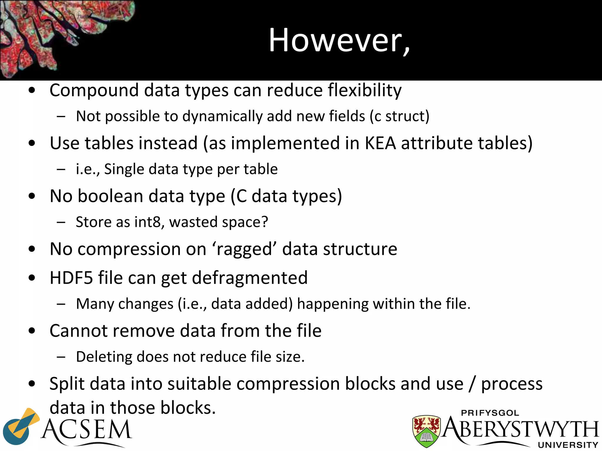
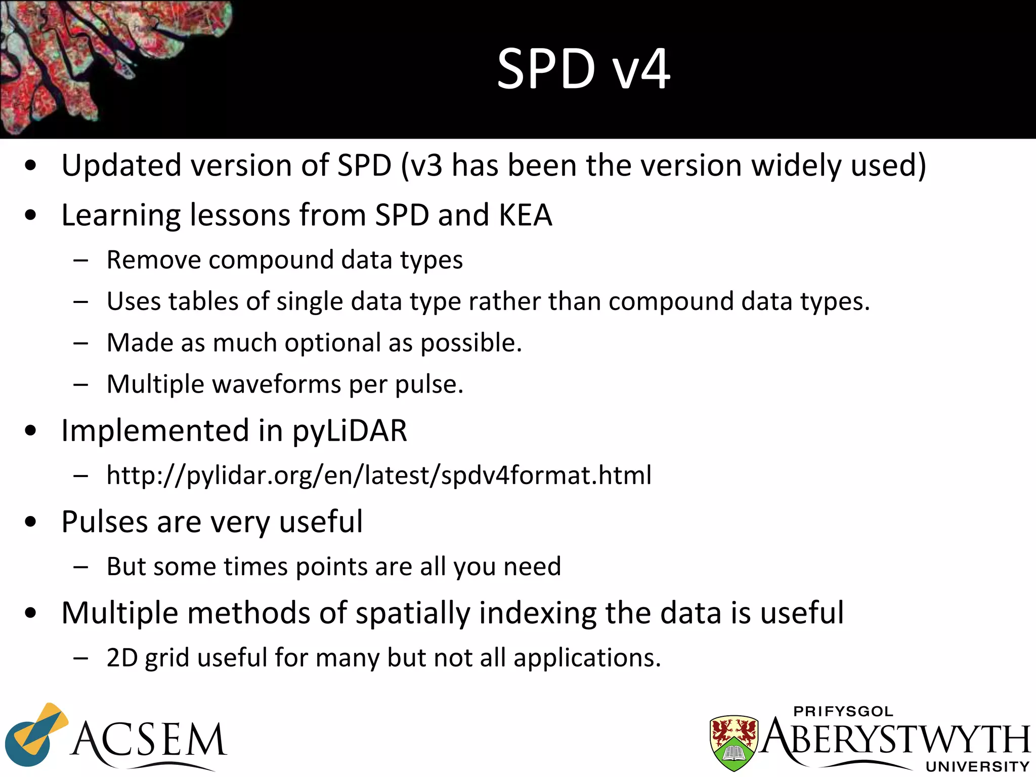
This document discusses two HDF5-based file formats for storing Earth observation data: 1. The Sorted Pulse Data (SPD) format stores laser scanning data including pulses and point data with attributes. It was created in 2008 and updated to version 4 to improve flexibility. 2. The KEA image file format implements the GDAL raster data model in HDF5, allowing large raster datasets and attribute tables to be stored together with compression. It was created in 2012 to address limitations of other formats. Both formats take advantage of HDF5 features like compression but also discuss some limitations and lessons learned for effectively designing scientific data formats.

1. @AU_EarthObs
SPD and KEA:
HDF5 based file formats for Earth
Observation
Pete Bunting1, John Armston2, Sam Gillingham3, Neil Flood4
1. Aberystwyth University, UK (pfb@aber.ac.uk)
2. University of Maryland, USA (armston@umd.edu)
3. Landcare Research, NZ (gillingham.sam@gmail.com)
4. Science Division, Queensland Government, Australia (neil.flood@dsiti.qld.gov.au)

2. Contents
• Sorted Pulse Data (SPD) Format
– For storing laser scanning data
• KEA Image File Format
– Implementation of the GDAL raster data
model.

3. SPD: Little History…
• The first version of ‘SPDLib’ was written in 2008
– ‘Sorted Point Data’, simply stored a 2D grid based index
alongside the points file.
• 2009 I was using a ENVI image file to store the header
information (as a 2 band image). Having multiple files per
datasets wasn’t ideal also LAS missing fields (e.g., height)
I wanted for processing.
– Colleague suggested looking at HDF5
• 2011 John Armston visited Aberystwyth with a set of full
waveform acquisitions for use in his PhD.
– ‘Sorted Pulse Data’ was born.

4. Why a Pulse?
Transmitted Received
Video created by John
Armston using SPDLib
Python binding.

5. SPD File Format
Pulse ID
GPSTime
Origin [X, Y, Z, H]
Index [X, Y]
Azimuth
Zenith
TransmitAmplitude
TransmitWidth
SourceID
Wavelength
NumberOfReturns
Returns
NumberOfTransmittedBins
TransmittedBins
NumberOfRecievedBins
RecievedBins
SPD Pulse
Point ID
GPSTime
Location [X, Y, Z, H]
Classification
Amplitude
Width
Range
Red
Green
Blue
WaveformOffset
SPD Point
Point ID
GPSTime
Location [X, Y, Z, H]
Classification
Amplitude
Width
Range
Red
Green
Blue
WaveformOffset
SPD Point
Point ID
GPSTime
Location [X, Y, Z, H]
Classification
Amplitude
Width
Range
Red
Green
Blue
WaveformOffset
SPD Point
Pulse ID
GPSTime
Origin [X, Y, Z, H]
Index [X, Y]
Azimuth
Zenith
TransmitAmplitude
TransmitWidth
SourceID
Wavelength
NumberOfReturns
Returns
NumberOfTransmittedBins
TransmittedBins
NumberOfRecievedBins
RecievedBins
SPD Pulse
Point ID
GPSTime
Location [X, Y, Z, H]
Classification
Amplitude
Width
Range
Red
Green
Blue
WaveformOffset
SPD Point
Point ID
GPSTime
Location [X, Y, Z, H]
Classification
Amplitude
Width
Range
Red
Green
Blue
WaveformOffset
SPD Point
Point ID
GPSTime
Location [X, Y, Z, H]
Classification
Amplitude
Width
Range
Red
Green
Blue
WaveformOffset
SPD Point
Pulse ID
GPSTime
Origin [X, Y, Z, H]
Index [X, Y]
Azimuth
Zenith
TransmitAmplitude
TransmitWidth
SourceID
Wavelength
NumberOfReturns
Returns
NumberOfTransmittedBins
TransmittedBins
NumberOfRecievedBins
RecievedBins
SPD Pulse
Point ID
GPSTime
Location [X, Y, Z, H]
Classification
Amplitude
Width
Range
Red
Green
Blue
WaveformOffset
SPD Point
Point ID
GPSTime
Location [X, Y, Z, H]
Classification
Amplitude
Width
Range
Red
Green
Blue
WaveformOffset
SPD Point
Point ID
GPSTime
Location [X, Y, Z, H]
Classification
Amplitude
Width
Range
Red
Green
Blue
WaveformOffset
SPD Point
Pulse ID
GPSTime
Origin [X, Y, Z, H]
Index [X, Y]
Azimuth
Zenith
TransmitAmplitude
TransmitWidth
SourceID
Wavelength
NumberOfReturns
Returns
NumberOfTransmittedBins
TransmittedBins
NumberOfRecievedBins
RecievedBins
SPD Pulse
Point ID
GPSTime
Location [X, Y, Z, H]
Classification
Amplitude
Width
Range
Red
Green
Blue
WaveformOffset
SPD Point
Point ID
GPSTime
Location [X, Y, Z, H]
Classification
Amplitude
Width
Range
Red
Green
Blue
WaveformOffset
SPD Point
Point ID
GPSTime
Location [X, Y, Z, H]
Classification
Amplitude
Width
Range
Red
Green
Blue
WaveformOffset
SPD Point
Pulse ID
GPSTime
Origin [X, Y, Z, H]
Index [X, Y]
Azimuth
Zenith
TransmitAmplitude
TransmitWidth
SourceID
Wavelength
NumberOfReturns
Returns
NumberOfTransmittedBins
TransmittedBins
NumberOfRecievedBins
RecievedBins
SPD Pulse
Point ID
GPSTime
Location [X, Y, Z, H]
Classification
Amplitude
Width
Range
Red
Green
Blue
WaveformOffset
SPD Point
Point ID
GPSTime
Location [X, Y, Z, H]
Classification
Amplitude
Width
Range
Red
Green
Blue
WaveformOffset
SPD Point
Point ID
GPSTime
Location [X, Y, Z, H]
Classification
Amplitude
Width
Range
Red
Green
Blue
WaveformOffset
SPD Point
Pulse ID
GPSTime
Origin [X, Y, Z, H]
Index [X, Y]
Azimuth
Zenith
TransmitAmplitude
TransmitWidth
SourceID
Wavelength
NumberOfReturns
Returns
NumberOfTransmittedBins
TransmittedBins
NumberOfRecievedBins
RecievedBins
SPD Pulse
Point ID
GPSTime
Location [X, Y, Z, H]
Classification
Amplitude
Width
Range
Red
Green
Blue
WaveformOffset
SPD Point
Point ID
GPSTime
Location [X, Y, Z, H]
Classification
Amplitude
Width
Range
Red
Green
Blue
WaveformOffset
SPD Point
Point ID
GPSTime
Location [X, Y, Z, H]
Classification
Amplitude
Width
Range
Red
Green
Blue
WaveformOffset
SPD Point
Pulse ID
GPSTime
Origin [X, Y, Z, H]
Index [X, Y]
Azimuth
Zenith
TransmitAmplitude
TransmitWidth
SourceID
Wavelength
NumberOfReturns
Returns
NumberOfTransmittedBins
TransmittedBins
NumberOfRecievedBins
RecievedBins
SPD Pulse
Point ID
GPSTime
Location [X, Y, Z, H]
Classification
Amplitude
Width
Range
Red
Green
Blue
WaveformOffset
SPD Point
Point ID
GPSTime
Location [X, Y, Z, H]
Classification
Amplitude
Width
Range
Red
Green
Blue
WaveformOffset
SPD Point
Point ID
GPSTime
Location [X, Y, Z, H]
Classification
Amplitude
Width
Range
Red
Green
Blue
WaveformOffset
SPD Point
Pulse ID
GPSTime
Origin [X, Y, Z, H]
Index [X, Y]
Azimuth
Zenith
TransmitAmplitude
TransmitWidth
SourceID
Wavelength
NumberOfReturns
Returns
NumberOfTransmittedBins
TransmittedBins
NumberOfRecievedBins
RecievedBins
SPD Pulse
Point ID
GPSTime
Location [X, Y, Z, H]
Classification
Amplitude
Width
Range
Red
Green
Blue
WaveformOffset
SPD Point
Point ID
GPSTime
Location [X, Y, Z, H]
Classification
Amplitude
Width
Range
Red
Green
Blue
WaveformOffset
SPD Point
Point ID
GPSTime
Location [X, Y, Z, H]
Classification
Amplitude
Width
Range
Red
Green
Blue
WaveformOffset
SPD Point

6. Sorted…
Indexing makes
processing faster
– Cartesian
– Spherical
– Polar
A)
B)
C)
X
Y
Azimuth
Zenith
Radius
Azimuth

7. SPD & HDF5

8. Why HDF5?
• Another file format…
– Not just another block of
binary you cannot do
anything with unless you
have a format definition.
• Fields can be logically
named and data types
defined and read from the
file.
– Self describing.
HDF5
Data
Header
Index
Quicklook Image
Pulses
Points
Received
Transmitted
Header Field 1
Header Field n
.
.
.
Bin Offset
Number of Pulses

9. Compression
• zlib compression is used by default
– Provided by HDF5 library
– Compression block size can be varied using SPD
header parameters
• File sizes are on average slight smaller than an
uncompressed LAS file but larger than LAZ.
– More complex data structures
– Two pieces of information pulse and point(s)

10. KEA: Little History…
• Created in 2012 and funded by Landcare Research, NZ.
• The problem:
“How to have large attribute tables of data alongside raster data?”
• Erdas Imagine format (HFA, *.img) supports attribute tables but compression is
only supported for 32bit file sizes (i.e., < 2Gb).
– Attribute tables are also uncompressed.
• BigTiff supports large raster imagery but not attribute tables.
• Initial implementation with a hdf5 file for attribute table with a separate image
file (e.g., tiff).
– This was untidy and having to keep track of multiple files is not desirable.
• “Why not just put the image in the HDF5 file with a gdal driver?”
– Result the KEA HDF5 schema.

11. Raster Storage: KEA file format
• HDF5 based image file format
• GDAL driver
– Therefore the format can be used in any GDAL
compatibly software (e.g., ArcMap)
• Support for large raster attribute tables
• zlib based compression
– Small file sizes
– 10 m SPOT mosaic of New Zealand ~5GB per
island (Each approx. 65000, 84000 pixels)
Bunting and Gillingham 2013

12. KEA File Structure
File Type
Number of
bands
GeneratorResolution
Rotation
Size
TL CoordVersion
WKT
Name: Value
Name: Value
Kea Image
Band 1
Band 2
Band n
Meta Data
Header
GCPs
GCPs
WKT
ATT
Image
Layer Type
Data Type
Description
Overviews
Meta Data
Name: Value
Name: Value
Overview 1
Overview 2
Overview n
Data
Header
Neighbours
Boolean Data Integer Data
String DataDouble Data
Size
Double Fields
Chunk Size
Integer FieldsBoolean Fields
String Fields
Neighbours
Band Mask Band Usage
• This structure is essentially
the GDAL raster data model.
• GDAL is defacto standard for
EO raster data I/O.
• Used in open source and
commercial software
(e.g., ESRI).
• We added a few addition for
our own needs.
• Attribute table has
concept of ‘neighbours’
to allow transversal of a
set of clumps (e.g.,
object oriented image
classification).

13. KEA Size and Speed

14. Is HDF5 a good base?
• Yes. - We’ve found it excellent.
– Coding is quick and relatively easy
– No worrying about Endian etc.
• Originally SPD was developed on PowerPC Mac.
– If used correctly compression is good, with little
overhead of the HDF5 structures
– Possible to make complex and flexible data
structures.
• However, it is the data structures in the file
rather the ‘file format’ that is important thing.

15. However,
• Compound data types can reduce flexibility
– Not possible to dynamically add new fields (c struct)
• Use tables instead (as implemented in KEA attribute tables)
– i.e., Single data type per table
• No boolean data type (C data types)
– Store as int8, wasted space?
• No compression on ‘ragged’ data structure
• HDF5 file can get defragmented
– Many changes (i.e., data added) happening within the file.
• Cannot remove data from the file
– Deleting does not reduce file size.
• Split data into suitable compression blocks and use / process
data in those blocks.

16. SPD v4
• Updated version of SPD (v3 has been the version widely used)
• Learning lessons from SPD and KEA
– Remove compound data types
– Uses tables of single data type rather than compound data types.
– Made as much optional as possible.
– Multiple waveforms per pulse.
• Implemented in pyLiDAR
– http://pylidar.org/en/latest/spdv4format.html
• Pulses are very useful
– But some times points are all you need
• Multiple methods of spatially indexing the data is useful
– 2D grid useful for many but not all applications.

17. Questions