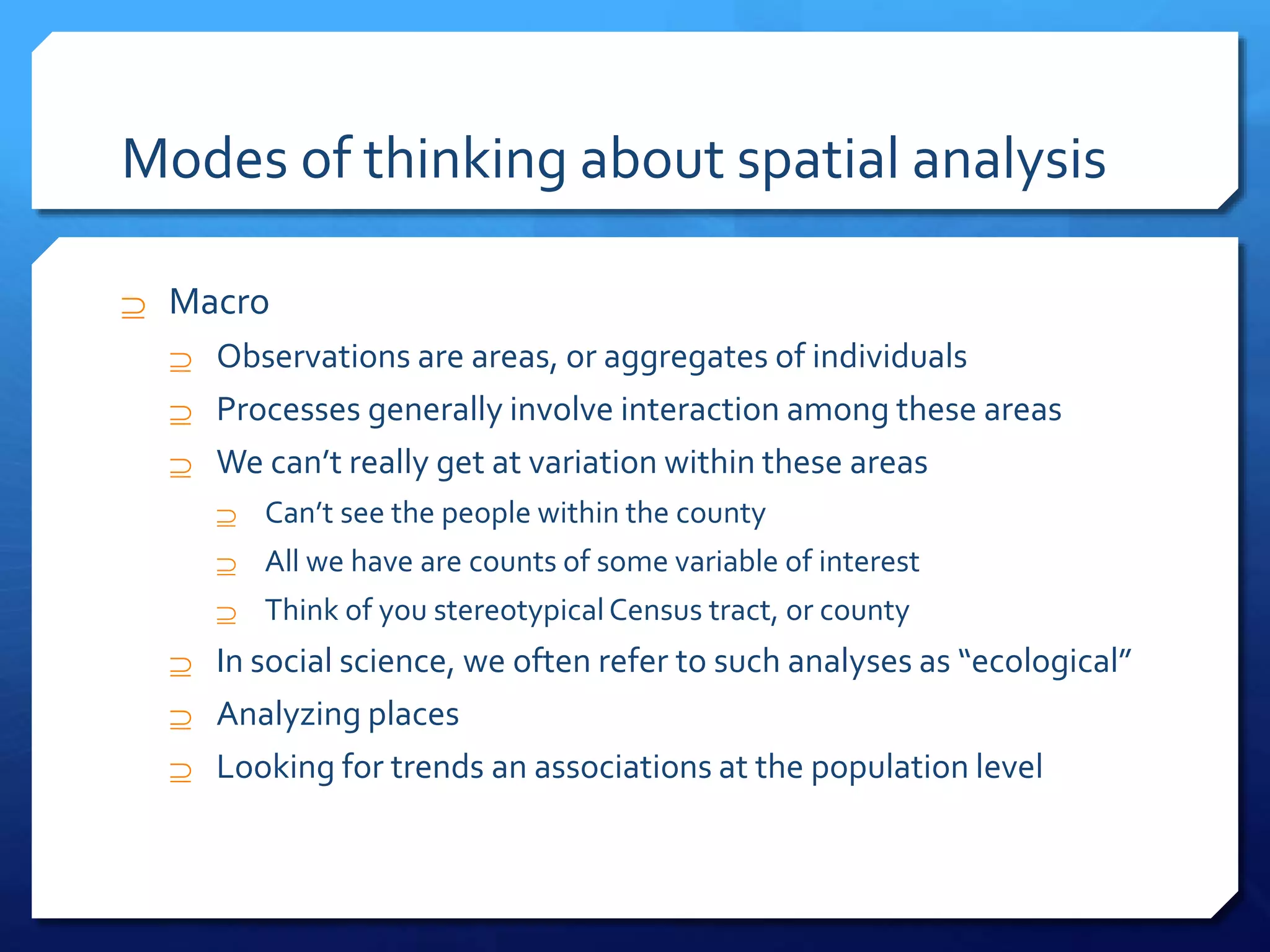
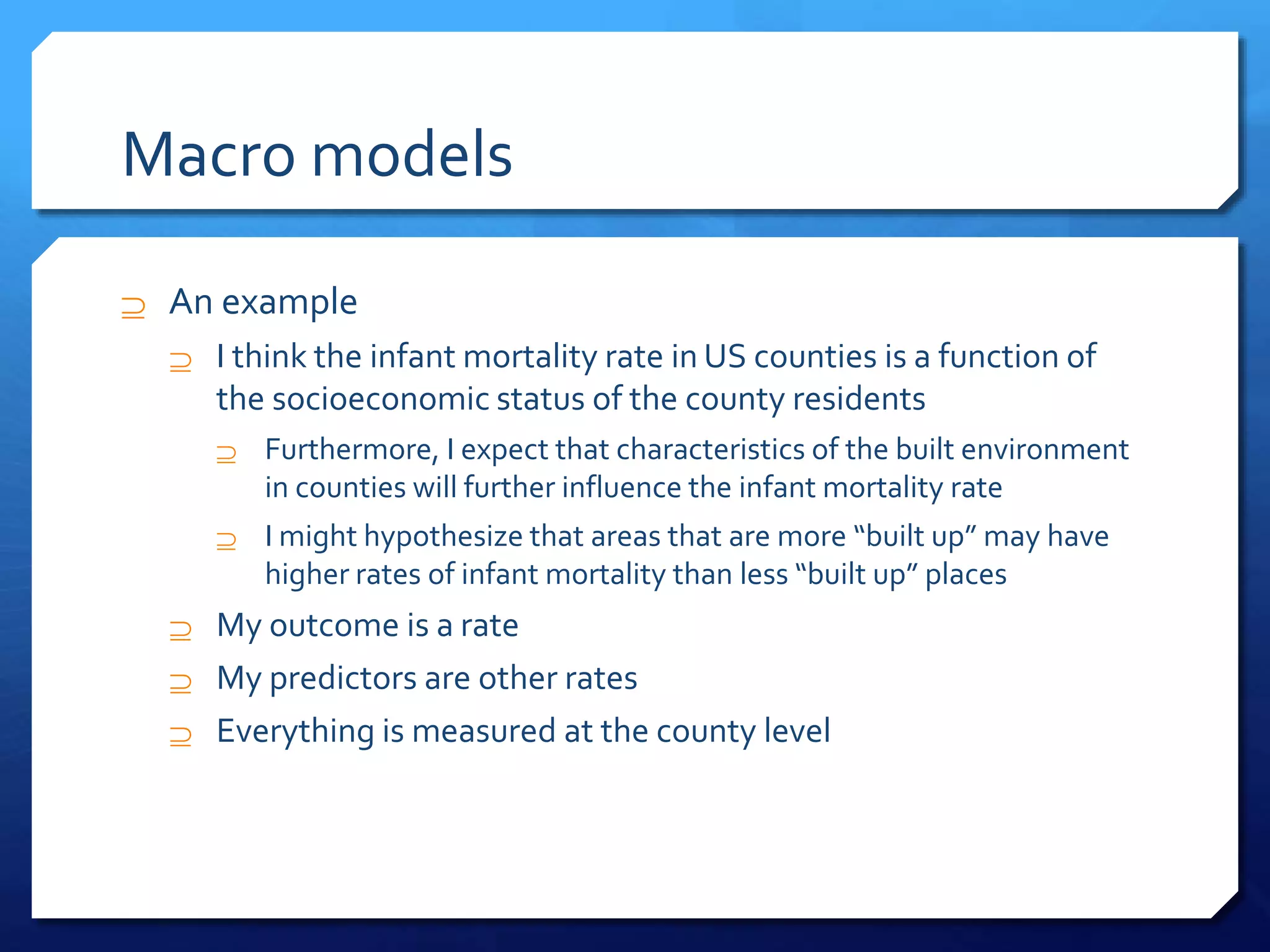
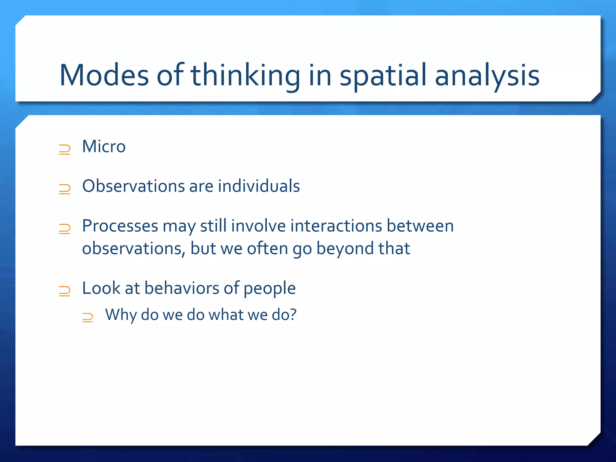
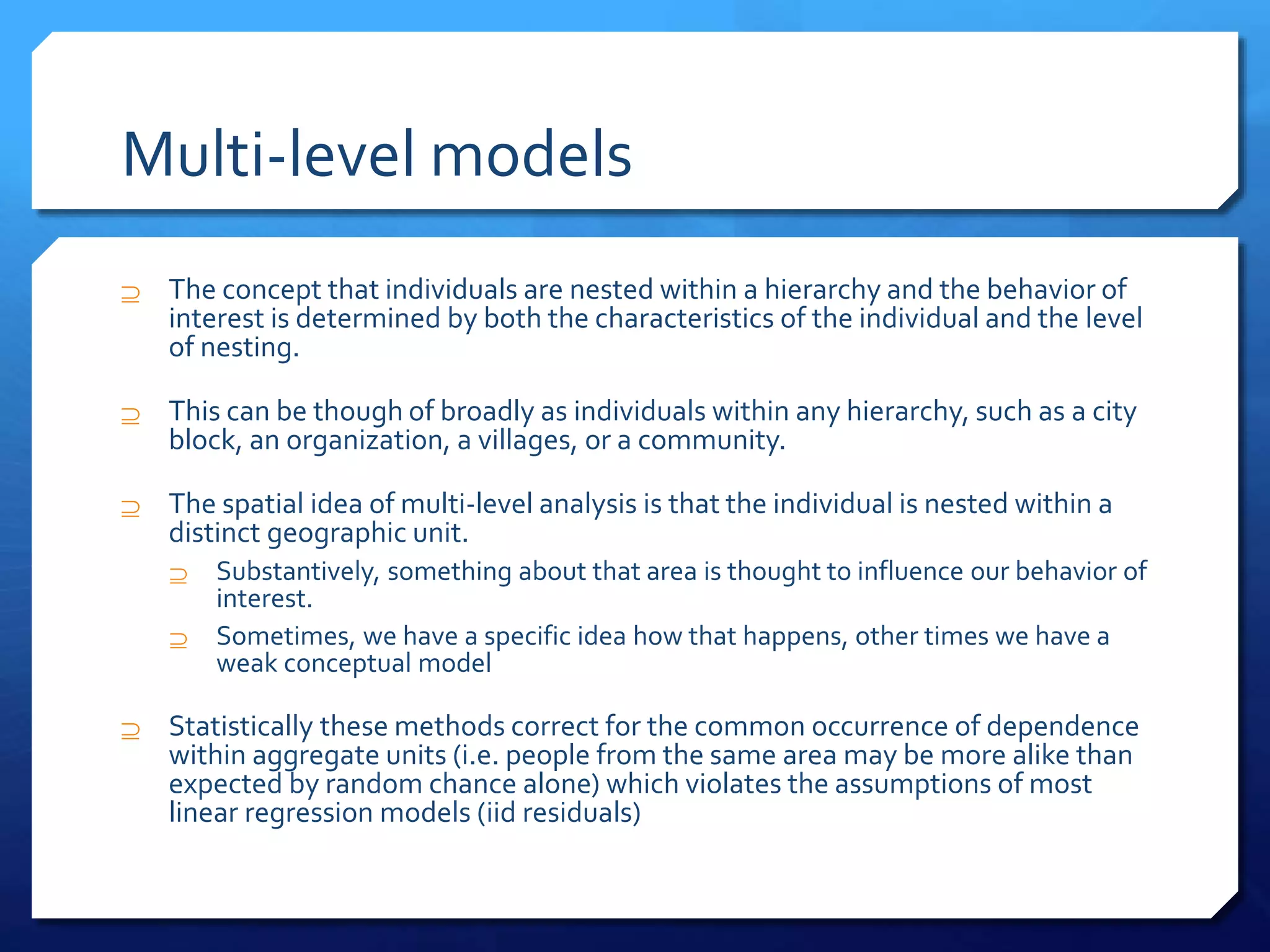
The purpose of this workshop is twofold. A primary goal is to provide researchers with a basic overview of spatial analysis. A secondary goal is to give attention to issues in GIS and spatial analysis that may be relevant to researchers planning to work with location data and unique geographies in confidential data sets in the Texas Census Research Data Center.
The workshop will consist of three sessions. Each session will be led by Dr. Corey Sparks, Assistant Professor at UTSA's College of Public Policy. Dr. Spark's research focuses on statistical demography, Geographic Information Systems and the application of modern statistical methods to problems in demography and health. His teaching interests focus on use and application of advanced statistical techniques including hazards analysis, multivariate methods and spatial statistics in human population analysis.
Multi agent paradigm for cognitive parameter based feature similarity for soc...eSAT Publishing House
IJRET : International Journal of Research in Engineering and Technology is an international peer reviewed, online journal published by eSAT Publishing House for the enhancement of research in various disciplines of Engineering and Technology. The aim and scope of the journal is to provide an academic medium and an important reference for the advancement and dissemination of research results that support high-level learning, teaching and research in the fields of Engineering and Technology. We bring together Scientists, Academician, Field Engineers, Scholars and Students of related fields of Engineering and Technology
Hybrid sentiment and network analysis of social opinion polarization icoictAndry Alamsyah
The rapid growth of social media and user generated contents (UGC) has provided a rich source of potentially relevant data. The problems arise on how to summarize those data to understand and transforming it into information. Twitter as one of the most popular social networking and micro-blogging service can be analyzed in terms of content produced with sentiment analysis. On the other hand, some types of networks can also be constructed to analyze the social network structure and network properties. This research intended to combine those content and structural approaches into hybrid approach for identifies social opinion polarization, this is in the form of conversation network. Sentiment analysis used to determine public sentiment, and social network analysis used to analyze the structure of the network, detecting communities and influential actors in the network. Using this hybrid approach, we have comprehensive understanding about social opinion polarization. As case study, we present real social opinion polarization about reclamation issue in Indonesia.
The world has moved on from 1973 when this paper appeared in the Journal of Sociology. At the core of human interaction is the desire to impart knowledge, that hasn't changed. If you want insight into how to strategically manage your networks to maximise knowledge exchange I have summarised the Granovetter's landmark paper here. The paper itself has been cited over 50,000 times and is seminal to the debate. You can access it here https://www.sciencedirect.com/science/article/pii/B9780124424500500250
The reason why we keep coming back to a paper like this is because no matter how far and fast we move forward, understanding why, is always an expression of interest and a depth of understanding
Social media network maps visualize the patterns of connection that form when people follow, reply and mention one another in Internet communication services like Twitter. When analyzed in aggregate collections of individual connections form web-like network structures.
As presented at the CASRO Digital Research Conference by Michael Lieberman of Multivariate Solutions.
Current trends of opinion mining and sentiment analysis in social networkseSAT Publishing House
IJRET : International Journal of Research in Engineering and Technology is an international peer reviewed, online journal published by eSAT Publishing House for the enhancement of research in various disciplines of Engineering and Technology. The aim and scope of the journal is to provide an academic medium and an important reference for the advancement and dissemination of research results that support high-level learning, teaching and research in the fields of Engineering and Technology. We bring together Scientists, Academician, Field Engineers, Scholars and Students of related fields of Engineering and Technology
Overview of analytic frameworks for complex adaptive systems and how those may apply to considerations of planning communities. Presented as graduate seminar in the School of Landscape Architecture at the University of New Mexico
Designs of epidemiological studies. Fundamentals of epidemiology for resident doctors and young researchers. Types of epidemiological studies, strengths and weaknesses. Language: Catalan
Predictive coding posits that neural systems make forward-looking predictions about incoming information.
Neural signals contain information not about the currently perceived stimulus, but about the difference
between the observed and the predicted stimulus. We propose to extend the predictive coding framework
from high-level sensory processing to the more abstract domain of theory of mind; that is, to inferences about
others’ goals, thoughts, and personalities. We review evidence that, across brain regions, neural responses
to depictions of human behavior, from biological motion to trait descriptions, exhibit a key signature of pre-
dictive coding: reduced activity to predictable stimuli. We discuss how future experiments could distinguish
predictive coding from alternative explanations of this response profile. This framework may provide an
important new window on the neural computations underlying theory of mind.
Spatial Reference Frames
Introduction to Spatial Planning
Exploratory Spatial Data Analysis Paper
Historical Features Of Spatial Data Essay
Research Paper On Spatial Inequality
Spatial Planning And Spatial Planning
Examples Of Visual-Spatial Abilities
Spatial And : Spatial Analysis
Spatial Memory
Edward T. Halls Four Spatial Zones
Spatial Specificity Analysis
Spatial Inequality
Definition Of Spatial Layout And Functionality
Spatial And Event-Based Design
Spatial Justice: The Concept Of Spatial Justice
The present study evaluates the possibility of spatial heterogeneity in the effects on municipal-level crime rates of both demographic and socio-economic variables. Geoggraphically weighted regression (GWR) is used for exploring spatial heterogeneity and confirms that place matters.
The emerging field of computational social science (CSS) is devoted to the pursuit of interdisciplinary social science research from an information processing perspective, through the medium of advanced computing and information technologies.
Presentation given at the HEA Social Sciences learning and teaching summit 'Exploring the implications of ‘the era of big data’ for learning and teaching'.
A blog post outlining the issues discussed at the summit is available via: http://bit.ly/1lCBUIB
APLIC 2014 - Social Observatories Coordinating NetworkAPLICwebmaster
NSF project looks to define social science research for the 21st century. The major objective of the SOCN is to continue exploration of ideas regarding the potential form and functioning of such a network of social observatories and to actively engage individuals and groups across the SBE research community in this process.
These slides are for my talk for the Somerville College Mathematics Reunion ("Somerville Maths Reunion", 6/24/17): http://www.some.ox.ac.uk/event/somerville-maths-reunion/
Patterns based information systems organization (@ InFuture 2015) Sergej Lugovic
Patterns-based Information Systems Organization
Sergej Lugović, Ivan Dunđer, Marko Horvat
Summary
The socio-technical systems research paradigm is about the complexity of real situations. It confronts us with the quest for variables that could provide us with insight into the behavior of such systems. Their behavior emerges according to internal system properties and adaptation of the system to external conditions.
In our view, behavioral patterns are one of those particular variables since machines can recognize them and their dynamics. Based on the synthesis of three different theoretical frameworks, this paper proposes a concept of patterns-based information system organization. The authors built the concept on the Deacon discussion of theory of information, Hofkirchner’s unified information theory and related system behavior, and Kelso’s explanation of pattern creation processes in self-organizing systems. All three researchers have included patterns in their theoretical proposal. According to this analysis of the existing theories and their synthesis, we conclude that in order to design machines that can automatically support new behavior, we have to analyze humans and machines as a complex whole with dynamic relationships and emerging patterns as a dependent variable of behavior. By developing this theoretical concept, we establish a departure point for future research and search for different variables that correlate with pattern formation.
The Complexity of Data: Computer Simulation and “Everyday” Social ScienceEdmund Chattoe-Brown
Although the existence of various forms of complexity in social systems is now widely recognised, this approach to explanation faces two major challenges that turn out to be intimately connected. The first is the existing conflict in social science between “micro” and “macro” styles of social explanation. The second is the relationship of complexity to the kind of data routinely collected in social science. In order to be accepted, complexity approaches need simultaneously to dodge the first conflict while making much better use of existing forms of data.
The first part of the talk will provide an introduction to the simulation approach and a discussion of various concepts in complexity with reference to simulation as a distinctive theory-building tool and methodology. The second part of the talk will develop these ideas in more depth using simulations by the author as case studies.
Similar to Spatial statistics presentation Texas A&M Census RDC (20)
These notes review fitting GLMs to aggregate data. Binomial, Poisson and Negative Binomial models are shown, with a few others. I also cover how to implement Moran Eigenvector filtering in a GLM. All data are for mortality rates for the state of Texas from the CDC Wonder.
Dem 7263 fall 2015 spatially autoregressive models 1Corey Sparks
These are notes for my Spatial Demography course. This lecture deals with the spatially autoregressive model. The model is reviewed and several applications are shown using real data for San Antonio, TX an US counties
Demography 7263 fall 2015 spatially autoregressive models 2Corey Sparks
This lecture describes alternative spatially autoregressive model specifications, and the use of specification testing. The model is reviewed and several applications are shown using real data for US counties
Recent research on residential segregation has focused on defining trends in areas outside of traditional metropolitan areas, including so-called new destinations and established immigrant gateways. Moreover a trend of decreasing black-white segregation between 1970 and 2009 has been described by recent work by Iceland and colleagues. In this paper, we go beyond the approach used in this recent work to investigate the county-level patterns of change in residential segregation between 1990 and 2010 using the most recent decennial census data available. We consider both black-white and Hispanic-Non-Hispanic patterns of segregation using measures of three dimensions of segregation: Evenness, Exposure and spatial clustering. Furthermore, we use tools of exploratory spatial data analysis and Geographic Information System (GIS) visualization to highlight areas of the country experiencing the most change over this period. This will allow us to see sub-regional trends in the dynamics of segregation, and understand the nature of segregation beyond the traditional black-white dichotomy, especially in areas of recent Hispanic immigration.
Sparks and Valencia PAA 2014 session107Corey Sparks
Intimate partner violence (IPV) is one of the most common forms of violence against women worldwide. The most recent WHO (2013) reports show that nearly one third (30%) of women reported ever experiencing either physical IPV, with regional figures as large as 38%. Risk factors exist at the individual, couple and ecological levels, but no systematic study of models at these various levels has been attempted. The goal of this analysis is to present a systematic evaluation of competing models of IPV risk. Using a Bayesian modeling framework, we compare models at various levels and evaluate their performance in terms of explaining IPV risk. In general, individual-centric models fit the data better than the couple-centric models, and the best fitting model considered woman’s and couple’s effects, plus heterogeneity at the region level. Overall, in the Peruvian setting, partner violence is largely a product of individual and couple-level dynamics.
This is a presentation I gave at Texas A&M University in November 2012. It is a talk that summarizes this publication: http://rd.springer.com/article/10.1007/s10708-011-9445-3
This is a presentation that we gave at the 2012 Population Association of America meeting in San Francisco, CA. In it, we describe a comparison between Bayesian county level poverty rate estimates and those of the SAIPE program of the US Census Bureau
San Antonio Food Insecurity AssessmentCorey Sparks
This is a presentation we gave at the first annual San Antonio Food Policy conference in May 2012. It goes through the results of a project funded by the city of San Antonio on assessing food insecurity in the city.
(May 29th, 2024) Advancements in Intravital Microscopy- Insights for Preclini...Scintica Instrumentation
Intravital microscopy (IVM) is a powerful tool utilized to study cellular behavior over time and space in vivo. Much of our understanding of cell biology has been accomplished using various in vitro and ex vivo methods; however, these studies do not necessarily reflect the natural dynamics of biological processes. Unlike traditional cell culture or fixed tissue imaging, IVM allows for the ultra-fast high-resolution imaging of cellular processes over time and space and were studied in its natural environment. Real-time visualization of biological processes in the context of an intact organism helps maintain physiological relevance and provide insights into the progression of disease, response to treatments or developmental processes.
In this webinar we give an overview of advanced applications of the IVM system in preclinical research. IVIM technology is a provider of all-in-one intravital microscopy systems and solutions optimized for in vivo imaging of live animal models at sub-micron resolution. The system’s unique features and user-friendly software enables researchers to probe fast dynamic biological processes such as immune cell tracking, cell-cell interaction as well as vascularization and tumor metastasis with exceptional detail. This webinar will also give an overview of IVM being utilized in drug development, offering a view into the intricate interaction between drugs/nanoparticles and tissues in vivo and allows for the evaluation of therapeutic intervention in a variety of tissues and organs. This interdisciplinary collaboration continues to drive the advancements of novel therapeutic strategies.
Seminar of U.V. Spectroscopy by SAMIR PANDASAMIR PANDA
Spectroscopy is a branch of science dealing the study of interaction of electromagnetic radiation with matter.
Ultraviolet-visible spectroscopy refers to absorption spectroscopy or reflect spectroscopy in the UV-VIS spectral region.
Ultraviolet-visible spectroscopy is an analytical method that can measure the amount of light received by the analyte.
Slide 1: Title Slide
Extrachromosomal Inheritance
Slide 2: Introduction to Extrachromosomal Inheritance
Definition: Extrachromosomal inheritance refers to the transmission of genetic material that is not found within the nucleus.
Key Components: Involves genes located in mitochondria, chloroplasts, and plasmids.
Slide 3: Mitochondrial Inheritance
Mitochondria: Organelles responsible for energy production.
Mitochondrial DNA (mtDNA): Circular DNA molecule found in mitochondria.
Inheritance Pattern: Maternally inherited, meaning it is passed from mothers to all their offspring.
Diseases: Examples include Leber’s hereditary optic neuropathy (LHON) and mitochondrial myopathy.
Slide 4: Chloroplast Inheritance
Chloroplasts: Organelles responsible for photosynthesis in plants.
Chloroplast DNA (cpDNA): Circular DNA molecule found in chloroplasts.
Inheritance Pattern: Often maternally inherited in most plants, but can vary in some species.
Examples: Variegation in plants, where leaf color patterns are determined by chloroplast DNA.
Slide 5: Plasmid Inheritance
Plasmids: Small, circular DNA molecules found in bacteria and some eukaryotes.
Features: Can carry antibiotic resistance genes and can be transferred between cells through processes like conjugation.
Significance: Important in biotechnology for gene cloning and genetic engineering.
Slide 6: Mechanisms of Extrachromosomal Inheritance
Non-Mendelian Patterns: Do not follow Mendel’s laws of inheritance.
Cytoplasmic Segregation: During cell division, organelles like mitochondria and chloroplasts are randomly distributed to daughter cells.
Heteroplasmy: Presence of more than one type of organellar genome within a cell, leading to variation in expression.
Slide 7: Examples of Extrachromosomal Inheritance
Four O’clock Plant (Mirabilis jalapa): Shows variegated leaves due to different cpDNA in leaf cells.
Petite Mutants in Yeast: Result from mutations in mitochondrial DNA affecting respiration.
Slide 8: Importance of Extrachromosomal Inheritance
Evolution: Provides insight into the evolution of eukaryotic cells.
Medicine: Understanding mitochondrial inheritance helps in diagnosing and treating mitochondrial diseases.
Agriculture: Chloroplast inheritance can be used in plant breeding and genetic modification.
Slide 9: Recent Research and Advances
Gene Editing: Techniques like CRISPR-Cas9 are being used to edit mitochondrial and chloroplast DNA.
Therapies: Development of mitochondrial replacement therapy (MRT) for preventing mitochondrial diseases.
Slide 10: Conclusion
Summary: Extrachromosomal inheritance involves the transmission of genetic material outside the nucleus and plays a crucial role in genetics, medicine, and biotechnology.
Future Directions: Continued research and technological advancements hold promise for new treatments and applications.
Slide 11: Questions and Discussion
Invite Audience: Open the floor for any questions or further discussion on the topic.
Nutraceutical market, scope and growth: Herbal drug technologyLokesh Patil
As consumer awareness of health and wellness rises, the nutraceutical market—which includes goods like functional meals, drinks, and dietary supplements that provide health advantages beyond basic nutrition—is growing significantly. As healthcare expenses rise, the population ages, and people want natural and preventative health solutions more and more, this industry is increasing quickly. Further driving market expansion are product formulation innovations and the use of cutting-edge technology for customized nutrition. With its worldwide reach, the nutraceutical industry is expected to keep growing and provide significant chances for research and investment in a number of categories, including vitamins, minerals, probiotics, and herbal supplements.
Deep Behavioral Phenotyping in Systems Neuroscience for Functional Atlasing a...Ana Luísa Pinho
Functional Magnetic Resonance Imaging (fMRI) provides means to characterize brain activations in response to behavior. However, cognitive neuroscience has been limited to group-level effects referring to the performance of specific tasks. To obtain the functional profile of elementary cognitive mechanisms, the combination of brain responses to many tasks is required. Yet, to date, both structural atlases and parcellation-based activations do not fully account for cognitive function and still present several limitations. Further, they do not adapt overall to individual characteristics. In this talk, I will give an account of deep-behavioral phenotyping strategies, namely data-driven methods in large task-fMRI datasets, to optimize functional brain-data collection and improve inference of effects-of-interest related to mental processes. Key to this approach is the employment of fast multi-functional paradigms rich on features that can be well parametrized and, consequently, facilitate the creation of psycho-physiological constructs to be modelled with imaging data. Particular emphasis will be given to music stimuli when studying high-order cognitive mechanisms, due to their ecological nature and quality to enable complex behavior compounded by discrete entities. I will also discuss how deep-behavioral phenotyping and individualized models applied to neuroimaging data can better account for the subject-specific organization of domain-general cognitive systems in the human brain. Finally, the accumulation of functional brain signatures brings the possibility to clarify relationships among tasks and create a univocal link between brain systems and mental functions through: (1) the development of ontologies proposing an organization of cognitive processes; and (2) brain-network taxonomies describing functional specialization. To this end, tools to improve commensurability in cognitive science are necessary, such as public repositories, ontology-based platforms and automated meta-analysis tools. I will thus discuss some brain-atlasing resources currently under development, and their applicability in cognitive as well as clinical neuroscience.
THE IMPORTANCE OF MARTIAN ATMOSPHERE SAMPLE RETURN.Sérgio Sacani
The return of a sample of near-surface atmosphere from Mars would facilitate answers to several first-order science questions surrounding the formation and evolution of the planet. One of the important aspects of terrestrial planet formation in general is the role that primary atmospheres played in influencing the chemistry and structure of the planets and their antecedents. Studies of the martian atmosphere can be used to investigate the role of a primary atmosphere in its history. Atmosphere samples would also inform our understanding of the near-surface chemistry of the planet, and ultimately the prospects for life. High-precision isotopic analyses of constituent gases are needed to address these questions, requiring that the analyses are made on returned samples rather than in situ.
Salas, V. (2024) "John of St. Thomas (Poinsot) on the Science of Sacred Theol...Studia Poinsotiana
I Introduction
II Subalternation and Theology
III Theology and Dogmatic Declarations
IV The Mixed Principles of Theology
V Virtual Revelation: The Unity of Theology
VI Theology as a Natural Science
VII Theology’s Certitude
VIII Conclusion
Notes
Bibliography
All the contents are fully attributable to the author, Doctor Victor Salas. Should you wish to get this text republished, get in touch with the author or the editorial committee of the Studia Poinsotiana. Insofar as possible, we will be happy to broker your contact.
Comparing Evolved Extractive Text Summary Scores of Bidirectional Encoder Rep...University of Maribor
Slides from:
11th International Conference on Electrical, Electronics and Computer Engineering (IcETRAN), Niš, 3-6 June 2024
Track: Artificial Intelligence
https://www.etran.rs/2024/en/home-english/
Comparing Evolved Extractive Text Summary Scores of Bidirectional Encoder Rep...
Spatial statistics presentation Texas A&M Census RDC
1. An Introduction to Spatial
Analysis in Socio-Economic and
Health Research
Corey S. Sparks, PhD
Department of Demography
The University ofTexas at San Antonio
2. Outline
1)What’s special about spatial?
Good news
Bad news
2) Modes of thinking about spatial analysis
Macro and Micro
3) Concepts of space
4) Spatial analysis is NOT statistics, but spatial statistics needs
spatial analysis
5) Using this for something meaningful
3. What’s special about spatial?
Spatial data have more information than ordinary data
Think of them as a triplet
Y, X, and Z, whereY is the variable of interest, X is some other
information that influencesY and Z is the geographic location
whereY occurred
If our data aren’t spatial, we don’t have Z
Spatial information is a key attribute of behavioral data
This adds a potentially interesting attribute to any data we
collect
4. What’s special about spatial?
Spatial data monkey with models
Most analytical models have assumptions, spatial structure can
violate these models
We typically want to jump into modeling, but without
acknowledging or handling directly, spatial data can make our
models meaningless
Some of the problems are..
5. The ecological fallacy
The tendency for aggregate data on a concept to show
correlations when individual data on a concept do not.
In general the effect of aggregation bias, whereby those
studying macro-level data try to make conclusions or
statements about individual-level behavior
This also is felt when you analyze data at a specific level, say
counties, your results are only generalizeable at that level,
not at the level of congressional districts, MSA’s or states.
The often-arbitrary nature of aggregate units also needs to
be considered in such analysis.
6. The modifiable area unit problem
(MAUP)
This is akin to the ecological fallacy and the notion of aggregation bias.
The MAUP occurs when inferences about data change when the spatial
scale of observation is modified.
i.e. at a county level there may be a significant association between income
and health, but at the state or national level this may become insignificant,
likewise at the individual level we may see the relationship disappear.
This problem also exists when we suspect that a characteristic of an
aggregate unit is influencing an individual behavior, but because the
level at which aggregate data are available, we are unable to properly
measure the variable at the aggregate level.
E.g. we suspect that neighborhood crime rates will the recidivism hazard
for a parolee, but we can only get crime rates at the census tract or county
level, so we cannot really measure the effect we want.
7. Spatial structure
Structure is the idea that your data have an organization to
them that has a specific spatial dimension
Think of a square grid
Each cell in the grid can be though of as being neighbors of
other cells base on their proximity, distance, direction, etc.
This structure generally influences data by making them non-
independent of one another
At best, you can have a correlation with your neighbor
At worst, your characteristics are a linear or nonlinear function
of your neighbors
8. Spatial heterogeneity
Spatial heterogeneity is the idea that characteristics of a
population or a sample vary by location
This can manifest itself by generating clusters of like
observations
Statistically, this is bad because many models assume
constant variance, but if like observations are spatially co-
incident, then variance is not constant
9. Modes of thinking about spatial analysis
Macro
Observations are areas, or aggregates of individuals
Processes generally involve interaction among these areas
We can’t really get at variation within these areas
Can’t see the people within the county
All we have are counts of some variable of interest
Think of you stereotypicalCensus tract, or county
In social science, we often refer to such analyses as “ecological”
Analyzing places
Looking for trends an associations at the population level
10. Macro models
An example
I think the infant mortality rate in US counties is a function of
the socioeconomic status of the county residents
Furthermore, I expect that characteristics of the built environment
in counties will further influence the infant mortality rate
I might hypothesize that areas that are more “built up” may have
higher rates of infant mortality than less “built up” places
My outcome is a rate
My predictors are other rates
Everything is measured at the county level
11. Modes of thinking in spatial analysis
Micro
Observations are individuals
Processes may still involve interactions between
observations, but we often go beyond that
Look at behaviors of people
Why do we do what we do?
12. Multi-level models
The concept that individuals are nested within a hierarchy and the behavior of
interest is determined by both the characteristics of the individual and the level
of nesting.
This can be though of broadly as individuals within any hierarchy, such as a city
block, an organization, a villages, or a community.
The spatial idea of multi-level analysis is that the individual is nested within a
distinct geographic unit.
Substantively, something about that area is thought to influence our behavior of
interest.
Sometimes, we have a specific idea how that happens, other times we have a
weak conceptual model
Statistically these methods correct for the common occurrence of dependence
within aggregate units (i.e. people from the same area may be more alike than
expected by random chance alone) which violates the assumptions of most
linear regression models (iid residuals)
13. Concepts of space
To start, let’s think about how to define space as a concept
i.e. what levels of space are important for human behavior?
Neighborhoods
Villages/towns
Social networks>social “space”
Households
Climatic zones
Political/administrative boundaries
14. What we really want to get at
What concept of space is important in my work?
That’s for you to decide
More often than not, as social scientists, we will undertake a macro
analysis or some form of nested micro analysis
At the macro level, we have to conceptualize the space of our units
Where are counties relative to one another
Is the spatial heterogeneity in my outcome at the county level
At the micro level, we have to justify why we believe the level of
nesting we can measure is in fact the right level in terms of our
outcome
Just because I know what MSA a child lives in, doesn’t tell me much about
the neighborhood in which they grew up
15. Spheres of social integration
Individuals exist within formal or more often informal
spheres of interaction.
You can think of these as areas where common ideas unite
people together, or the range (meaning distance) of social
norms.
Common ideology often unites individuals into groups and
groups into larger aggregates, look at the concept of
nationalism for example.
They can likewise have a strictly a-spatial representation, such
as a belief network.
16. Some parting thoughts about space
Realization that human behavior is a dynamic process, not a static
phenomena
Use of the cross-section as opposed to the cohort (longitudinal
data) or with respect to changes in the neighborhood.
Defining “meaningful” neighborhoods, not just available sampling
areas, how do individuals interact within these areas?
How do individuals interact with their neighborhood?
Ideas of agency and how an individual is an agent of change
Do people choose neighborhoods?Or are some chosen by the
neighborhoods they are born into, or only the ones they can afford?
17. Context or Composition?
Is it the places where people live that is important? (Context)
Or
Is it the nature of the people that live in the place?
(Composition)
Again, when justifying a spatially oriented analysis, these
things need to be addressed
18. Spatial analysis is NOT statistics
Enter the GIS
GIS is the manager of spatial information
Goes beyond the realm of relational databases by incorporating the
spatial context of all data
Uses this as the overarching infrastructure for organizing
information
The use of space as a tool
The GIS allows us to edit, merge, split, add, delete all types of
information based purely on the spatial location of the data
But, it is not statistics!
19. GIS operations as spatial analysis
We use the GIS to help us manage and visualize spatial data
There are thousands of specific tools offered in a standard GIS
We can organize the tools of spatial analysis by what type of data
they use:
Point patterns
Areas (polygons)
Images (raster)
Interactions
Networks
Sure I’m missing something
20. Spatial statistics needs spatial analysis
1)Without spatial analysis, we would miss out on the
interactions between our spatial information
Unable to construct important variables for statistical analysis
2) Without spatial analysis, we would be limited in our
visualization of our data, and our results
From maps to 3-D visualizations
21. Wrap Up
Spatial data is special
For better or for worse
Ignoring spatial structure can invalidate models
24. Exploratory Spatial DataAnalysis
What is ESDA?
In exploratory data analysis, we are looking for trends and patterns
in data
We are working under the assumption that the more one knows
about the data, the more effectively it may be used to develop,
test and refine theory
This generally requires we follow two principles: skepticism and
openness
25. One should be skeptical of measures that summarize data, since
they can conceal or misrepresent the most informative aspects of
data,
and..
We must be open to patterns in the data that we did not expect to
find, because these can often be the most revealing outcomes of
the analysis.
We must avoid the temptation to automatically jump to the
confirmatory model of data analysis.
26. The confirmatory model says: Do my data confirm the hypothesis
that X causesY.
We would normally fit a linear model (or something close to it) and
use summary measures (means and variances) to test if the
pattern we observe in the data is real.
The exploratory model says,
To the contrary, “What do the data I have tell me about the
relationship between X andY. This lends to a much more open
range of alternative explanations
27. The principle of EDA is explained best in the simple model:
Data = smooth + rough
The smooth bit is the underlying simplified structure of a set of observations.
This is the straight line that we expect a relationship to follow in linear
regression for example, or the smooth curve describing the distribution of
data: the pattern or regularity in the data.
You can also think of the smooth as a central parameter of a distribution, the
mean or median for example
The rough is the difference between our actual data, and the smooth. This
can be measured as the deviation of each point from the mean.
Outliers, for example are very rough data, they have a large difference from
the central tendency in a distribution, where all the other data points tend to
clump
28. Doing some ESDA
We will use new tools (namelyGeoDa) to do some Spatial EDA.
The way GeoDa differs from traditional ways of viewing data (on paper,
or with summary statistics), is that it goes beyond presenting the data, to
visualizing the data.
Data visualization is a dynamic process that incorporates multiple views
of the same information,
i.e. we can examine a histogram that is linked to a scatter plot that is
linked to a map to visualize the distribution of a single variable, how it is
related to another and how it is patterned over space.
We can also do what is called brushing the data, so we can select subsets
of the information and see if, there are distinct subsets of the data that
have different relational or spatial properties. This allows us to really
visualize how the processes we study unfolds over space and allows us to
see locations of potentially influential observations.
29. Some examples of ESDA items
Histograms
Boxplots
Scatter plots
Parallel coordinate plots
Area statistics/Local statistics
30. Histograms
Histograms are useful
tools for representing the
distribution of data
They can be used to judge
central tendency (mean,
median, mode), variation
(standard deviation,
variance), modality
(unimodal or multi-
modal), and graphical
assessment of
distributional
assumptions (Normality)
31. Box Plots
Box plots (or box and whisker
plots) are another useful tool for
examining the distribution of a
variable
You can visualize the 5 number
summary of a variable
Miniumum, Maximum, lower
quartile, Median, and upper
quartile
Upper
Quartile
Median
Lower
Quartile
Maximum
Minimum
IQR
32. Scatter Plots
Scatterplots show
bivariate relationships
This can give you a visual
indication of an
association between two
variables
Positive association
(positive correlation)
Negative association
(negative correlation)
Also allows you to see
potential outliers
(abnormal observations)
in the data
Slight
positive
association
Potential Outlier
33. Parallel Coordinate
Plots
Parallel coordinate
plots allow for
visualization of the
association between
multiple variables
(multivariate)
Each variable is
plotted according to
its “coordinates” or
values
34. Local Statistics
Local statistics allow
you to see how the
mean, or variation, of
a variable varies over
space
You can generate a
local statistic by
weighting an ordinary
statistic by some kind
of spatial weight
Example ->
Property crime in San
Antonio,TX
35. Global vs. Local Statistics
By global we imply that one statistic is used to adequately summarize
the data
i.e. the mean or median
Or, a regression model that is suitable for all areas in the data
Local statistics are useful when the process you are studying varies over
space,
i.e. different areas have different local values that might cluster together to
form a local deviation from the overall mean
Or a regression model that accounts for the same level of variation in the
outcome in all locations
36. Autocorrelation
This can occur in either space or time
Really boils down to the non-independence between neighboring
values
The values of our independent variable (or our dependent
variables) may be similar because
Our values occur
closely in time (temporal autocorrelation)
closely in space (spatial autocorrelation)
37. Preliminaries to assessing autocorrelation
Basic Assessment of Spatial Dependency
Before we can model the dependency in spatial data, we must
first cover the ideas of creating and modeling neighborhoods in
our data.
By neighborhoods, I mean the clustering or connectedness of
observations
The exploratory methods we will cover depend on us knowing
how our data are arranged in space, who is next to who.
This is important (as we will see later) because most correlation
in spatial data tends to die out as we get further away from a
specific location (Tobler’s law)
38. Tobler's first law of geography
WaldoTobler (1970) suggested the “jokingly” first law of
geography
“Everything is related to everything else, but near things are more
related than distant things”
We can see this better in graphical form: We expect the
correlation between the attributes of two points to diminish as the
distance between them grows
39. One thing about autocorrelation
Autocorrelation is
typically a local process
Meaning it typically
dies out as distance
between observations
increase
plot(exp(-.05*seq(1:100)), type="l", lwd=2,
ylab="Correlation", xlab="Distance")
40. W
To identify which observations are close to one another, we useW
W is the spatial weight matrix
Square n by n matrix with 1/0 entries identifying if any two
observations are spatial neighbors
How is this constructed?
There are two typical ways in which we measure spatial
relationships
Distance and contiguity
41. In a distance based connectivity method, features (generally
points) are considered to be contiguous if they are within a given
radius of another point.The radius is really left up to the researcher
to decide.
Likewise, we can calculate the distance matrix between a set of
points
This is usually measured using the standard Euclidean distance
Where x and y are coordinates (lat/long) of the point or polygon in
question, this is the as the crow flies distance
Distance based neighbors
42. More on distances
There are lots of distance measures
Manhattan distances
d = |x1 – x2| + |y1- y2|
These are city-block distances
We can use these distances to create a neighborhood of points
using certain criteria
43. Who is who's neighbor
There are many different criteria for deciding if two observations
are neighbors
Generally two observations must be within a critical distance, d, to
be considered neighbors.
This is the Minimum distance criteria, and is very popular.
This will generate a matrix of binary variables describing the
neighborhood.
We can also describe the neighborhoods in a continuous weighting
scheme based on the distance between them
Inverse Distance Weight wij=
1
dij
or
Inverse Squared Distance Weight wij=
1
dij
2
44. Contiguity/PolygonAdjacency
Polygons are contiguous if they share common topology, like
an edge (line segment) or a vertex (point)
Neighborhoods are created based on which observations are
judged “contiguous”
This is generally the best way to treat polygon features
Distances aren’t typically used for polygons for several
reasons
Spacing of observations
What centroid? Is it a good measure?
45. • Rook adjacency
• Neighbors must share
a line segment
• Queen adjacency
• Neighbors must share
a vertex or a line
segment
• If polygons share these
boundaries (based on the
specific definition: rook or
queen), they are given a
weight of 1 (adjacent), else
they are given a value 0,
(nonadjacent)
46. Order of adjacency
Observation of interest
First order neighbors (Rook)
Second Order neighbors (Rook)
Observation of interest
First order neighbors (Queen)
Second Order neighbors (Queen)
First and second order
Rook adjacency
First and second order
Queen adjacency
47. What does a spatial weight matrix look like?
Set of polygons
SpatialWeight Matrix,W
48. StandardizedW
Most times, in analytical work,W is standardized
Typically this is done by dividing each 1/0 element in the row
by the sum of the row, which would yield this matrix:
Polygon 1 2 3 4
1 0 0.5 0.5 0
2 0.5 0 0 0.5
3 0.5 0 0 0.5
4 0 0.5 0.5 0
49. Forms of autocorrelation
Positive autocorrelation
This means that a feature is positively associated with the values
of the surrounding area (as defined by the spatial weight matrix),
high values occur with high values, low with low
Negative autocorrelation
This means that a feature is negatively associated with the values
of the surrounding area (as defined by the spatial weight matrix),
high with low, low with high
The (probably) most popular global autocorrelation statistic is
Moran’s I
51. Moran's I
Measure of standardized spatial autocovariance
with xi being the value of the attribute at location i, xj being the value of the
attribute at location j,
S0 is the sum of all spatial weights
wij is the weight for location ij (0 if they are not neighbors, 1 otherwise)
Approximately bound on 0,1 with a similar interpretation as a Pearson or
Spearman correlation
52. Geary’s C
Measure of spatial covariance
with xi being the value of the attribute at location i, xj being the
value of the attribute at location j,
S0 is the sum of all spatial weights
wij is the weight for location ij (0 if they are not neighbors, 1
otherwise)
Bound on 0,2
0 to 1 = positive autocorrelation
1= no autocorrelation
1 to 2=negative autocorrelation
53. Getis – Ord G
Unlike I and C, the interpretation of G focuses on whether
high values of x tend to cluster with other high values of x
The measure is directional
Likewise, low with low
54. Local Moran’s I
We can also describe the local trends in autocorrelation in our
data by constructing local versions of our autocorrelation
statistics
Each has a local version
This is useful to see where the autocorrelation is high or low
within our data
Goes beyond the global statistics to help us visualize where in
our data associations are strong
55. How do you determine if the data
are in a cluster?
This is done via the Moran scatterplot.
If an observation is in the top right quadrant of the plot =
high-high
Bottom left quadrant = low – low
Top left quadrant = high – low
Bottom right quadrant = low-high
56. Moran scatterplot (univariate)
It is sometimes useful to visualize the relationship between the actual
values of the dependent variable and their lagged values. This is the so
called
Moran scatterplot
Lagged values are the average value of the surrounding neighborhood
around location I
lag(x) = wij*x = Wx in matrix terms
The Moran scatterplot shows the association between the observation of
interest and its neighborhood's average value
The variables are generally plotted as z-scores, to avoid scaling issues
58. Local Moran
cluster map
Significant high
neighborhood
deprivation on
the west, east
and south sides
Significant low
neighborhood
deprivation on
the north side
59. Spatially lagged values
If we have a value xi at location i and a spatial weight matrix wij
describing the spatial neighborhood around location i, we can find the
lagged value of the variable by:
Wxi = xi * wij
This calculates what is effectively, the neighborhood average value in
locations around location i, often stated x-i
60.
61. Moran scatterplot (Bivariate)
We can also compare the lagged value of one variable verses the
value of another variable
Wy versus x
This is the so-called “multivariate Moran scatterplot”
It is often useful in so-called space-time analysis, when we
compare the value of one variable measured at two different time
points. This will show the correlation between space over time.
63. What these methods tell you
Moran's I is a descriptive statistic
It simply indicates if there is spatial association/autocorrelation
in a variable
Local Moran's I tells you if there is significant localized
clustering of the variable
Where spatial clusters and what type of cluster is present
66. Goals
To show how you can use R, software that is free and
available in the RDC to:
1) Perform interesting spatially-oriented analysis
2) Merge spatial data from multiple sources
Spatial join
3)Visualize results from a spatial analysis much as you would in
a GIS environment
Without a GIS!
67. Residential Segregation and Crime in San
Antonio,TX
Four data sources:
American Community Survey 5 year summary file
Census tract level
Census 2000 Summary File 1
Block level
SanAntonio Police Department call data
Point data based on geocoded addresses
All calls received by the SAPD in a year
CensusTIGER file for SanAntonio tracts
68. Methods
1)Merge ACS calculated fields to shapefile based on tract FIPS code
2) Perform spatial join of crimes to tracts
Count # of crimes in each tract
3) Create a thematic map of the crime rate using quantile breaks
4) Create tract-level indices of residential segregation by
aggregating up from the block level
Merge these to the shapefile
5) Perform ESDA using Local Moran statistics on the segregation
index and crime rate
71. Spatial Disease Mapping
Application to crime data, but principles remain the same
Trying to locate areas of excess disease risk
Finding spatial clusters of disease
Kulldorff and Nagarwalla’s Spatial Scan Statistic
DCluster library
Modeling spatial relative risk
Bayesian Hierarchical Regression
Posterior model summaries
INLA library
Approximate Bayesian inference by Integrated Nested Laplace
Approximation
Great for Gaussian random field models
72. Methods
Spatial Scan Statistic
Constructs a grid over the area, centered on each observation
Using a set radius (defined based on a proportion of the
population size at risk), a circle is created on each point
The likelihood function
is used, and the area with the maximum value of the function is
the most likely cluster of cases
Allows for ranked clusters (primary, secondary, etc)
74. Basics of Bayesian Modeling
Some statistical ideas:
Likelihood
Usually we have some data that we assume follow some distribution
For counts, maybeY ~ Poisson(λ)
L (y, λ) is the joint probability distribution of the data and the
parameters
The model likelihood is the product of this distribution for all
observations
We get the estimate of λ that is the most likely to have generated our
data (y)
Maximum likelihood estimate of λ
This is traditional statistics
75. Bayesian statistics
Now, lets consider the case where we have some knowledge
about λ, say we believe it comes from a certain distribution,
so :
λ ~ Gamma(α,β)
And we can either assume some value for these parameters
(α=β=1) or allow them to also come from some distribution
α~Exp(u) ,β~Exp(p)
Why a Gamma distn? Because Gamma is >0, and we know θ is
>0 because it is a relative risk
76. Combining information
When we combine the likelihood and the prior, we form what
is called the posterior distribution
Thus we have BayesTheorem which in the continuous case
is:
Which states, the posterior distribution of θ, conditional on y
is the product of the likelihood and the prior distribution of θ
77. The denominator in Bayes theorem is a constant, and this is
generally written as:
Which says the posterior is proportional to the likelihood
times the prior
79. Simple Models
Let’s now consider a simple realistic model
yi~Poisson(ei θi)
Assume the usual log link function
log (θi) = C1+C2
C1=a0+x’β
Linear Poisson regression with intercept
C2=other terms
Could add random effect - > this would be like an individual frailty model, or a
group frailty model or a random intercept model
Generally this is called a Generalized Linear Mixed Model
Now we just need to code it up!
80. Mapping and spatial modeling
We just achieved a better, more accurate SMR map with a
simple Poisson model with a random effect
This model “drew strength” from counties with good data to
help smooth counties with poor data, but it didn’t account for
correlation between neighboring counties
We can also build a model that includes a spatially correlated
random effect between counties
Spatially smoothed rates
81. Building a Spatial Model
Take a Poisson-Lognormal model
y~Pois(ei θi)
θi=α+ x’β + ui
What if we introduce more interesting structure on u?
A common form of spatial correlation structure is the CAR model, or
also called the Besag model
This is:
82. More models
Another model that is commonly used in practice is the
convolution model, or the Besag,York and Mollie model
y~Pois(ei θi)
θi=α+ x’β + ui + vi
Where now ui is a correlated heterogeneity (CH) term and vi
is an Uncorrelated Heterogeneity (UH) term
84. Why Use R?
R is free (So are GeoDA and QGIS)
R is available in the RDC (So are GeoDA and QGIS)
R is extremely capable and flexible (So is QGIS)
R is a scripting and statistical language (Neither GeoDA or
QGIS are)
R is one stop shopping for many geospatial techniques
Spatial joins, projections, data merging, raster analysis, vector
operations