SPARQL Query Processing Techniques using Structural
Information of RDF Graphs in Relational RDF Store
Seoul National University
Internet Database Lab.
Kisung Kim
2013. 11. 22
Ph.D Defense Presentation
OUTLINE
• Introduction
– Motivation
– Existing Approaches
– Contributions
• R3F: RDF Triple Filtering for SPARQL Query Processing
• RP-Index: RDF Path index for Triple Filtering
• RG-index: RDF Graph index for Triple Filtering
• Conclusion & Future Work
2/39
INTRODUCTION (1/8)
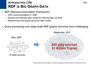
RDF IS BIG GRAPH DATA
• RDF (Resource Description Framework)
– W3C recommendation in 1998
– General and flexible data model for sharing data via Web
– Schema-less and graph-structure data model
• Query processing over large-scale RDF graphs becomes more challenging
Linking Open Data cloud diagram, by Richard Cyganiak and Anja Jentzsch. http://lod-cloud.net/
September, 2011
May, 2007
12 data sources
3/39
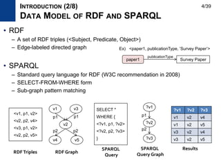
• RDF
– A set of RDF triples (<Subject, Predicate, Object>)
– Edge-labeled directed graph
• SPARQL
– Standard query language for RDF (W3C recommendation in 2008)
– SELECT-FROM-WHERE form
– Sub-graph pattern matching
SPARQL
Query
INTRODUCTION (2/8)
DATA MODEL OF RDF AND SPARQL
RDFTriples
<v1, p1, v2>
<v2, p2, v4>
<v3, p1, v2>
<v2, p2, v5>
v2
v4
v1
RDF Graph
?v1
?v2
?v3
SPARQL
Query Graph
SELECT *
WHERE {
<?v1, p1, ?v2>
<?v2, p2, ?v3>
}
v3
v5
?v1 ?v2 ?v3
v1 v2 v4
v1 v2 v5
v3 v2 v4
v3 v2 v5
Results
Ex) <paper1, publicationType, ‘Survey Paper’>
paper1 Survey Paper
publicationType
p1 p1
p2 p2
p1
p2
4/39
Relational RDF Store Graph RDF Store
Storage Relational table
Adjacent list
Mainly In-memory
Query
Processing
Relational operator
Join and scan
Sub-graph isomorphism algorithm
System
Jena [WWW2004] , Sesame [ISWC2002],
Oracle [VLDB2005], SW-store [VLDBJ2009],
RDF-3X [VLDBJ2010]
GRIN [AAAI2007], Dogma [ISWC2009],
PIG [SemData2010], gStore [VLDBJ2013]
Pros
Batch processing using Join operator
Large-scale RDF processing [VLDB2012]
Reduce search space of the graph
traversal using the graph structure
Cons Not using the graph structure
Not scalable
Inappropriate for large-scale
processing
INTRODUCTION (3/8)
TWO TYPES OF RDF STORES
5/39
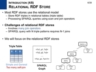
• Most RDF stores use the relational model
– Store RDF triples in relational tables (triple table)
– Processing SPARQL queries using scan and join operators
• Challenges of relational RDF stores
– Involves many join operators
– SPARQL query with N triple patterns requires N-1 joins
• We will focus on the relational RDF stores
INTRODUCTION (4/8)
RELATIONAL RDF STORE
Scan
p1
Scan
p2
Join1
Scan
p3
Join2
SPARQL
Graph
S P O
TripleTable
Too many self-join
Simple and General
<?v1, p1, ?v2>
<?v2, p2, ?v3>
….
<?vn, pn, ?vn+1>
Scan
pn
Joinn-1
….
6/39
• Storage approaches
– Clustered property table
– Jena [WWW2004] , Sesame [ISWC2002], Oracle [VLDB2005]
– Cluster properties which are accessed together frequently
– Sorted triple tables (multiple indexing)
– SW-store [VLDBJ2009], RDF-3X [VLDBJ2010]
– Store triples as sorted in a column-oriented store or clustered B+ trees
ID Name age gender
Clustered PropertyTable
S P O
SortedTripleTable
S
S P O
P
S P O
O
INTRODUCTION (5/8)
EXISTING RELATIONAL RDF STORE
Reduce joins
Limited flexibility, Cluster decision
Null value, Multi value
Fast retrieval of matching triples
Fast merge join
Storage overhead, update
7/39
• Handling intermediate results approaches
– Finding optimal plan
– Static and traditional approach
– Propose RDF-specific histograms
– RDF-3X [VLDBJ2010], Characteristics set [ICDE2011], ARQ [WWW2008]
– Dynamic filtering method
– Build dynamic filters and use subsequent operators
– U-SIP [SIGMOD2009]
• Existing methods do not exploit graph structure of RDF graphs
Scan
p1
Scan
p2
Merge Join
Scan
p3
Hash Join
Next Information
Domain Filter
Scan
p1
Scan
p2
Merge Join
Scan
p3
Hash Join
Finding Optimal Plan (static) Dynamic Filtering Method
INTRODUCTION (6/8)
EXISTING RELATIONAL RDF STORE
8/39
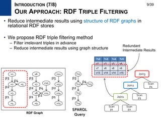
• Reduce intermediate results using structure of RDF graphs in
relational RDF stores
• We propose RDF triple filtering method
– Filter irrelevant triples in advance
– Reduce intermediate results using graph structure
INTRODUCTION (7/8)
OUR APPROACH: RDF TRIPLE FILTERING
v3
v4
v2 v5
v1
v8
v9
v7 v10
v6
v11 v14
v15
v13
v12
p3
p2
p1
p4
p3
p2
p1 p2
p4
p3
p2
p1
RDF Graph
Scan
p1
Scan
p2
Join1
Scan
p3
Join2
Scan
p4
Join3
?v2 ?v3 ?v4 ?v5
v2 v3 v3 v4
v7 v8 v8 v9
v13 v14 v14 v15
Redundant
Intermediate Results
?v3
?v4
?v2 ?v5
?v1
p3
p2
p4
p1
SPARQL
Query
9/39
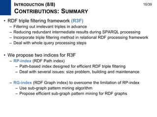
• RDF triple filtering framework (R3F)
– Filtering out irrelevant triples in advance
– Reducing redundant intermediate results during SPARQL processing
– Incorporate triple filtering method in relational RDF processing framework
– Deal with whole query processing steps
• We propose two indices for R3F
– RP-index (RDF Path index)
– Path-based index designed for efficient RDF triple filtering
– Deal with several issues: size problem, building and maintenance
– RG-index (RDF Graph index) to overcome the limitation of RP-index
– Use sub-graph pattern mining algorithm
– Propose efficient sub-graph pattern mining for RDF graphs
INTRODUCTION (8/8)
CONTRIBUTIONS: SUMMARY
10/39
OUTLINE
• Introduction
• R3F: RDF Triple Filtering for SPARQL Query Processing
– Motivation
– Overview of R3F
– Three components of R3F
• RP-Index: RDF Path Index for R3F
• RG-index: RDF Graph index for Triple Filtering
• Conclusion & Future Work
11/39
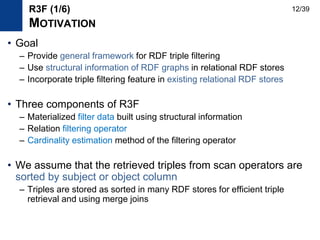
• Goal
– Provide general framework for RDF triple filtering
– Use structural information of RDF graphs in relational RDF stores
– Incorporate triple filtering feature in existing relational RDF stores
• Three components of R3F
– Materialized filter data built using structural information
– Relation filtering operator
– Cardinality estimation method of the filtering operator
• We assume that the retrieved triples from scan operators are
sorted by subject or object column
– Triples are stored as sorted in many RDF stores for efficient triple
retrieval and using merge joins
R3F (1/6)
MOTIVATION
12/39
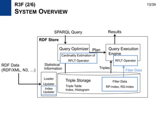
Query Execution
Engine
Query Optimizer
SPARQL Query
Plan
Statistical
Information
Triple Storage
Triples
Results
RDF Store
Filter Data
RP-index, RG-index
RFLT Operator
Cardinality Estimation of
RFLT Operator
Loader
Updater
RDF Data
(RDF/XML, N3, …)
Triple Table
Index, HistogramIndex
Updater
R3F (2/6)
SYSTEM OVERVIEW
Filter Data
13/39
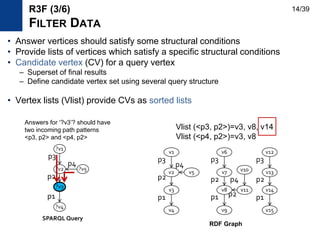
• Answer vertices should satisfy some structural conditions
• Provide lists of vertices which satisfy a specific structural conditions
• Candidate vertex (CV) for a query vertex
– Superset of final results
– Define candidate vertex set using several query structure
• Vertex lists (Vlist) provide CVs as sorted lists
?v3
?v4
?v2 ?v5
?v1
p3
p2
p4
p1
SPARQL Query
v3
v4
v2 v5
v1
v8
v9
v7 v10
v6
v11 v14
v15
v13
v12
p3
p2
p1
p4
p3
p2
p1 p2
p4
p3
p2
p1
Answers for ‘?v3’? should have
two incoming path patterns
<p3, p2> and <p4, p2>
Vlist (<p3, p2>)=v3, v8, v14
Vlist (<p4, p2>)=v3, v8
R3F (3/6)
FILTER DATA
RDF Graph
14/39
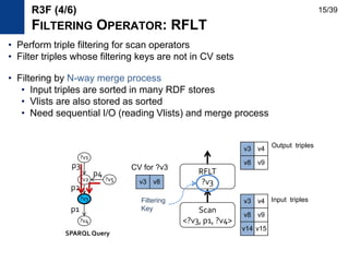
• Perform triple filtering for scan operators
• Filter triples whose filtering keys are not in CV sets
• Filtering by N-way merge process
• Input triples are sorted in many RDF stores
• Vlists are also stored as sorted
• Need sequential I/O (reading Vlists) and merge process
Scan
<?v3, p1, ?v4>
RFLT
?v3v3 v8
v3 v4
v8 v9
v14 v15
?v3
?v4
?v2 ?v5
?v1
p3
p2
p4
p1
SPARQL Query
CV for ?v3
v3 v4
v8 v9
R3F (4/6)
FILTERING OPERATOR: RFLT
Filtering
Key
Input triples
Output triples
15/39
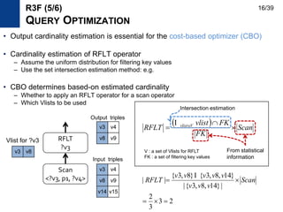
• Output cardinality estimation is essential for the cost-based optimizer (CBO)
• Cardinality estimation of RFLT operator
– Assume the uniform distribution for filtering key values
– Use the set intersection estimation method: e.g.
• CBO determines based-on estimated cardinality
– Whether to apply an RFLT operator for a scan operator
– Which Vlists to be used
Scan
<?v3, p1, ?v4>
RFLT
?v3
v3 v8
Vlist for ?v3
R3F (5/6)
QUERY OPTIMIZATION
v3 v4
v8 v9
v14 v15
v3 v4
v8 v9
Input triples
Output triples
  Scan
FK
FKvlist
RFLT Vvlist


 
V : a set of Vlists for RFLT
FK : a set of filtering key values
Intersection estimation
From statistical
information
23
3
2
|}14,8,3{|
}14,8,3{}8,3{
||

 Scan
vvv
vvvvv
RFLT

16/39
R3F (6/6)
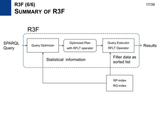
SUMMARY OF R3F
RP-index
RG-index
Filter data as
sorted list
Query Optimizer
SPARQL
Query
Optimized Plan
with RFLT operator
Query Executor
RFLT Operator
Results
Statistical information
R3F
17/39
OUTLINE
• Introduction
• R3F: RDF Triple Filtering
• RP-Index: RDF Path Index for R3F
– Design of RP-Index
– Size Problem
– Experimental Results
• RG-index: RDF Graph index for Triple Filtering
• Conclusion & Future Work
18/39
• Motivation
– Design an index to provide vertex lists having a specific path pattern
– Efficient and updatable index
• Related work: path-based index
– DataGuide [VLDB1997], 1-index [ICDT1999], A(k)-index [ICDE2002],
D(k)-index [SIGMOD2003], M(k)-index [ICDE2004]
– Provide a concise summary of the original data for query processing
– Handle size problem by store every vertex one time in the index
• Our goal is to provide filter data efficiently
– Vertices can be stored several times and stored as sorted
– We deal with the size problem differently
RP-INDEX (1/7)
MOTIVATION AND RELATED WORK
19/39
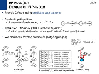
• Provide CV sets using predicate path patterns
• Predicate path pattern
– A sequence of predicate: e.g. <p1, p2, p3>
• Definition: RP-index (RDF Database D, maxL)
– A set of <ppath, Vlist(ppath)>, where ppath exists in D and |ppath| ≤ maxL
• We also index reverse predicates (outgoing edges)
v3
v4
v2 v5
v1
v8
v9
v7 v10
v6
v11 v14
v15
v13
v12
p3
p2
p1
p4
p3
p2
p1 p2
p4
p3
p2
p1
?v3
?v4
?v2 ?v5
?v1
p3
p2
p4
p1
SPARQL Query
CV for ?v3 =
Vlist(<p3, p2>) ∩ Vlist(p4, p2) =
{v3, v8}
RP-INDEX (2/7)
DESIGN OF RP-INDEX
?v1 ?v2 ?v3
p1 p2
?v4
p3
RDF Graph
Vlist (<p1>) = v4
Vlist (<p2>) = v3
Vlist (<p3>) = v2
Vlist (<p4>) = v2
Vlist (<p1R>) = v3
Vlist (<p2R>) = v2
Vlist (<p3R>) = v1
Vlist (<p4R>) = v5
Vlist (<p2, p1>) = v4
Vlist (<p3, p2>) = v3
Vlist (<p4, p2>) = v3
Vlist (<p1R,p2R>) = v2
Vlist (<p2R,p3R>) = v1
Vlist (<p2R,p4R>) = v5
Vlist(<p2,p2R>)=v11
Vlist(<p3,p4R>)=v5
RP–index (D, 2) with reverse predicate
20/39
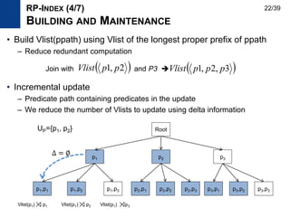
• Exponential number of predicate paths
, where |P| is the number of predicates
• Solution
– Choose effective predicate path for filtering
• Two criteria for choosing predicate paths
– Discriminative predicate path: use a replaceable predicate path
– Frequent predicate path: infrequent Vlists are rarely used
)||( 1
maxL
i
i
PO
r1 r2 r3 r4 r5 r6 r7 r2 r3 r4 r6 r7
Vlist(<p2, p3>) Vlist(<p1,p2,p3>)
|Vlist(<p2,p3>)| / |Vlist(<p1,p2,p3>)| = 5/7 = 0.71
∩
RP-INDEX (3/7)
SIZE PROBLEM OF RP-INDEX
If discriminative ratio is 0.7, then
Vlist(<p1, p2, p3>) is not stored
If minimum frequency is 7, then
Vlist(<p1, p2, p3>) is not stored
r2 r3 r4 r6 r7
Vlist(<p1,p2,p3>)
Discriminative Predicate Path Frequent Predicate Path
21/39
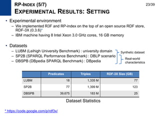
• Build Vlist(ppath) using Vlist of the longest proper prefix of ppath
– Reduce redundant computation
• Incremental update
– Predicate path containing predicates in the update
– We reduce the number of Vlists to update using delta information
RP-INDEX (4/7)
BUILDING AND MAINTENANCE
 3,2,1 pppVlist 2,1 ppVlistJoin with and P3 
Root
p1 p2 p3
p1,p1 p1,p2 p1,p3 p2,p1 p2,p2 p2,p3 p3,p1 p3,p2 p3,p3
UP={p1, p2}
Vlist(p1) p1 Vlist(p1) p2 Vlist(p1) p3
22/39
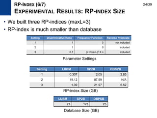
• Experimental environment
– We implemented R3F and RP-index on the top of an open source RDF store,
RDF-3X (0.3.6)*
– IBM machine having 8 Intel Xeon 3.0 GHz cores, 16 GB memory
• Datasets
– LUBM (Leihigh University Benchmark) : university domain
– SP2B (SPARQL Performance Benchmark) : DBLP scenario
– DBSPB (DBpedia SPARQL Benchmark) : DBpedia
Predicates Triples RDF-3X Size (GB)
LUBM 18 1,335 M 77
SP2B 77 1,399 M 123
DBSPB 39,675 183 M 25
Dataset Statistics
RP-INDEX (5/7)
EXPERIMENTAL RESULTS: SETTING
Synthetic dataset
Real-world
characteristics
* https://code.google.com/p/rdf3x/
23/39
• We built three RP-indices (maxL=3)
• RP-index is much smaller than database
Setting LUBM SP2B DBSPB
1 0.307 2.05 2.85
2 19.12 87.99 N/A
3 1.39 21.97 6.52
Setting Discriminative Ratio Frequency Function Reverse Predicate
1 1 0 not included
2 1 0 included
3 0.7 (l-1/maxL)2 X n included
Parameter Settings
RP-index Size (GB)
RP-INDEX (6/7)
EXPERIMENTAL RESULTS: RP-INDEX SIZE
LUBM SP2B DBPSB
77 123 25
Database Size (GB)
24/39
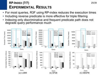
• For most queries, R3F using RP-index reduces the execution times
• Including reverse predicate is more effective for triple filtering
• Indexing only discriminative and frequent predicate path does not
degrade query performance much
RP-INDEX (7/7)
EXPERIMENTAL RESULTS
(a) LUBM (b) SP2B (C) DBSPB
25/39
OUTLINE
• Introduction
• R3F: RDF Triple Filtering using RG-index
• RP-Index: RDF Path Index for R3F
• RG-index: RDF Graph index for Triple Filtering
– Motivation
– Design of RG-index
– Building RG-index
– Evaluaion Results
• Conclusion & Future Work
26/39
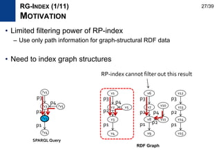
• Limited filtering power of RP-index
– Use only path information for graph-structural RDF data
• Need to index graph structures
RP-index cannot filter out this result
?v3
?v4
?v2 ?v5
?v1
p3
p2
p4
p1
SPARQL Query
v3
v4
v2 v5
v1
v8
v9
v7 v10
v6
v11 v14
v15
v13
v12
p3
p2
p1
p4
p3
p2
p1 p2
p4
p3
p2
p1
RG-INDEX (1/11)
MOTIVATION
RDF Graph
27/39
• Graph index
– Graph-transactional setting (many small graphs)
– GraphGrep [PODS2002], gIndex [SIGMOD2004], C-tree [ICDE2006],
QuckSI [VLDB2008], Tale [ICDE2008]
– A single large graph
– GraphQL [SIGMOD2008], GADDI [EDBT2009], SPath [VLDB2010]
– For reducing the search space of the graph traversal
– Non-trivial to apply to relational RDF stores
• Subgraph pattern mining
– Graph-transactional setting
– gSpan [ICDM2002], Gaston [KDD2004]
– A single large graph
– HSIGRAM, VSIGRAM [JDMKD2005]
– Not scalable for large RDF graphs
– We need to adapt existing algorithm for RDF graphs
RG-INDEX (2/11)
RELATED WORK
28/39
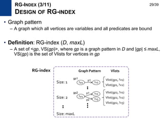
• Graph pattern
– A graph which all vertices are variables and all predicates are bound
• Definition: RG-index (D, maxL)
– A set of <gp, VS(gp)>, where gp is a graph pattern in D and |gp| ≤ maxL,
VS(gp) is the set of Vlists for vertices in gp
Graph Pattern
?v1 ?v2Size: 1
?v1
?v2
Size: 2
Size: maxL
?v3
VlistsRG-index
Vlist(gp1, ?v1)
RG-INDEX (3/11)
DESIGN OF RG-INDEX
p1
p1
p2
gp1
gp2
Vlist(gp1, ?v2)
Vlist(gp2, ?v1)
Vlist(gp2, ?v2)
Vlist(gp2, ?v3)
29/39
• Use subgraph mining due to the size problem of RG-index
– Indexing only frequent subgraph patterns  Frequent subgraph mining
• Adapt gSpan [Yan and Han, ICDM ’02] algorithm for RDF graphs
• gSpan
– Transactional setting
– Depth-first pattern growth approach
– Use anti-monocity property of support
– Use DFS encoding and edge extension
to prevent duplicate pattern generation
RG-INDEX (4/11)
BUILDING RG-INDEX USING SUBGRAPH MINING
size-2
size-1
size-maxL
Edge extension
pruning infrequent
or duplicate pattern
30/39
• Pattern representation
– Use DFS code and extend it to directed edge-label graph [SIGKDD2003]
• Support definition
– Should satisfy anti-monotonicity property for efficient mining
– Most mining algorithm use MIS (maximum independent set) approach,
which is NP-hard for the single large setting
– We use support definition in [Bringmann and Nijssen, PAKDD ‘08]
as minimum matching vertex number
– Very efficient to compute and upper-bound of MIS approaches
(mining more patterns)
|)),((|min)sup( vGVlistG Vv
RG-INDEX (5/11)
ADAPTING GSPAN FOR RDF GRAPHS
31/39
• Redundant subgraph patterns
– Graph patterns with same Vlists
– Graphs having non-trivial automorphisms
• Compute occurrences of graph pattern
– Exploit depth-first style pattern generation similarly to VSIGRAM [JDMKD2005]
– Store all occurrences of a pattern to compute child patterns
– Store occurrences from root to a leaf (depth-first approach)
– We propose efficient occurrence computation method
RG-INDEX (6/11)
ADAPTING GSPAN FOR RDF GRAPHS
Redundant
patterns
32/39
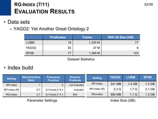
• Data sets
– YAGO2: Yet Another Great Ontology 2
• Index build
RG-INDEX (7/11)
EVALUATION RESULTS
Predicates Triples RDF-3X Size (GB)
LUBM 18 1,335 M 77
YAGO2 93 37 M 9
SP2B 77 1,399 M 123
Dataset Statistics
Setting YAGO2 LUBM SP2B
RP-index 341 MB 1.4 GB 1.3 GB
RP-index (R) 2.3 G 1.7 G 3.1 GB
RG-index 880 MB 1.1 G 1.3 GB
Setting
Discriminative
Ratio
Frequency
Function
Reverse
Predicate
RP-index 1 0 not included
RP-index (R) 0.7 (l-1/maxL)2 X n included
RG-index 0.7 (l-1/maxL)2 X n N/A
Parameter Settings Index Size (GB)
33/39
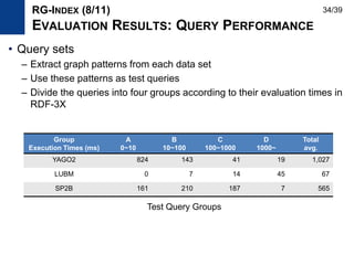
• Query sets
– Extract graph patterns from each data set
– Use these patterns as test queries
– Divide the queries into four groups according to their evaluation times in
RDF-3X
RG-INDEX (8/11)
EVALUATION RESULTS: QUERY PERFORMANCE
Test Query Groups
Group
Execution Times (ms)
A
0~10
B
10~100
C
100~1000
D
1000~
Total
avg.
YAGO2 824 143 41 19 1,027
LUBM 0 7 14 45 67
SP2B 161 210 187 7 565
34/39
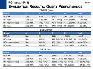
Group A B C D Total
RDF-3X 2.76 29.02 244.62 1383.42 108.65
RP-index 2.38 (13%) 25.2 (13%) 182.72 (25%) 555.42 (59%) 76.08 (30%)
RP-index (reverse) 2.39 (13%) 25.2 (13%) 153.92 (37%) 127 (91%) 61.06 (43.8%)
RG-index 2.33 (15%) 16.39 (43%) 122.8 (49%) 106.85 (92%) 44.34 (59.19%)
RG-INDEX (9/11)
EVALUATION RESULTS: QUERY PERFORMANCE
Group A B C D Total
RDF-3X N/A 59 444.6 2158.6 1548.8
RP-index N/A 58 (1%) 441. 6 (0.6%) 2126.9 (0.1%) 1526.8 (1%)
RP-index (reverse) N/A 50 (15%) 420 (5%) 1274.1 (40%) 946.4 (38%)
RG-index N/A 50 (15%) 406 (8%) 1250.2 (42%) 929.7 (40%)
Group A B C D Total
RDF-3X 3.53 34.18 240.43 16671.261 325.62
RP-index 2.75 (22%) 11.83 (65%) 94.73 (60%) 9194.21 (44%) 177.73 (45%)
RP-index (reverse) 3.00 (15%) 17.82 (47%) 79.78 (66%) 4747.26 (71%) 95.90 (70%)
RG-index 2.32 (34%) 8.65 (74%) 27.60 (88%) 581.36 (96%) 14.92 (95%)
SP2B (ms)
LUBM (ms)
YAGO2 (ms)
35/39
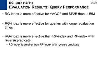
• RG-index is more effective for YAGO2 and SP2B than LUBM
• RG-index is more effective for queries with longer evaluation
times
• RG-index is more effective than RP-index and RP-index with
reverse predicate
– RG-index is smaller than RP-index with reverse predicate
RG-INDEX (10/11)
EVALUATION RESULTS: QUERY PERFORMANCE
36/39
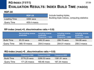
Frequency=1000 Frequency=2000 Frequency=4000
Build Time 5776.25 secs 3290.53 secs 1381.61 secs
Query Time 171.25 msecs 169.46 msec 187.34 msecs
Not including reverse
predicates
including reverse
predicates
(frequency = 1000)
including reverse
predicates
(frequency = 2000)
including reverse
predicates
(frequency = 4000)
Build Time 93.33 secs 449.33 secs 299.79 secs 164.88 secs
Query Time 368.19 msecs 254.0 msecs 254.01 msecs 258.3 msecs
RDF-3X
Loading Time 4264 secs
Query Time 409.4 msecs
RP-index (maxL=5, discriminative ratio = 0.8)
RG-index (maxL=5 , discriminative ratio = 0.8)
Include loading triples,
Building triple indices, computing statistics
RG-INDEX (11/11)
EVALUATION RESULTS: INDEX BUILD TIME (YAGO2)
37/39
RDF-3X
CONCLUSIONS
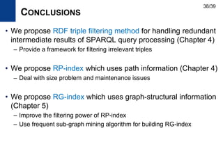
• We propose RDF triple filtering method for handling redundant
intermediate results of SPARQL query processing (Chapter 4)
– Provide a framework for filtering irrelevant triples
• We propose RP-index which uses path information (Chapter 4)
– Deal with size problem and maintenance issues
• We propose RG-index which uses graph-structural information
(Chapter 5)
– Improve the filtering power of RP-index
– Use frequent sub-graph mining algorithm for building RG-index
38/39
FUTURE WORK
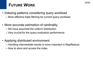
• Indexing patterns considering query workload
– More effective triple filtering for current query workload
• More accurate estimation of cardinality
– We have assumed the uniform distribution
– Very crucial for the query evaluation performance
• Applying distributed environment
– Handling intermediate results is more important in MapReduce
– How to store and access the index
39/39
PAPERS
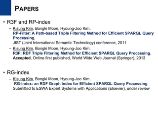
• R3F and RP-index
– Kisung Kim, Bongki Moon, Hyoung-Joo Kim,
RP-Filter: A Path-based Triple Filtering Method for Efficient SPARQL Query
Processing,
JIST (Joint International Semantic Technology) conference, 2011
– Kisung Kim, Bongki Moon, Hyoung-Joo Kim,
R3F: RDF Triple Filtering Method for Efficient SPARQL Query Processing,
Accepted, Online first published, World Wide Web Journal (Springer), 2013
• RG-index
– Kisung Kim, Bongki Moon, Hyoung-Joo Kim,
RG-index: an RDF Graph Index for Efficient SPARQL Query Processing
Submitted to ESWA Expert Systems with Applications (Elsevier), under review
Thank You
Any Questions?
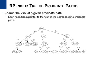
RP-INDEX: TRIE OF PREDICATE PATHS
• Search the Vlist of a given predicate path
– Each node has a pointer to the Vlist of the corresponding predicate
paths
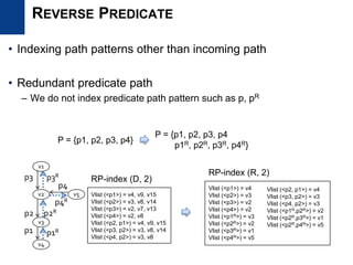
• Indexing path patterns other than incoming path
• Redundant predicate path
– We do not index predicate path pattern such as p, pR
v3
v4
v2 v5
v1
p3
p2
p1
p4
RP-index (R, 2)
Vlist (<p1>) = v4
Vlist (<p2>) = v3
Vlist (<p3>) = v2
Vlist (<p4>) = v2
Vlist (<p1R>) = v3
Vlist (<p2R>) = v2
Vlist (<p3R>) = v1
Vlist (<p4R>) = v5
P = {p1, p2, p3, p4}
P = {p1, p2, p3, p4
p1R, p2R, p3R, p4R}
p3R
p2R
p1R
p4R
Vlist (<p2, p1>) = v4
Vlist (<p3, p2>) = v3
Vlist (<p4, p2>) = v3
Vlist (<p1R,p2R>) = v2
Vlist (<p2R,p3R>) = v1
Vlist (<p2R,p4R>) = v5
REVERSE PREDICATE
RP-index (D, 2)
Vlist (<p1>) = v4, v9, v15
Vlist (<p2>) = v3, v8, v14
Vlist (<p3>) = v2, v7, v13
Vlist (<p4>) = v2, v8
Vlist (<p2, p1>) = v4, v9, v15
Vlist (<p3, p2>) = v3, v8, v14
Vlist (<p4, p2>) = v3, v8
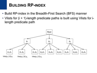
BUILDING RP-INDEX
• Build RP-index in the Breadth-First Search (BFS) manner
• Vlists for (i + 1)-length predicate paths is built using Vlists for i-
length predicate path
Root
p1 p2 p3
p1,p1 p1,p2 p1,p3 p2,p1 p2,p2 p2,p3 p3,p1 p3,p2 p3,p3
Vlist(p1) p1 Vlist(p1) p2 Vlist(p1) p3
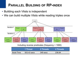
PARALLEL BUILDING OF RP-INDEX
• Building each Vlists is independent
• We can build multiple Vlists while reading triples once
1 Thread 2 Threads 4 Threads
Build Time 503.43 secs 349 secs 238.84
Including reverse predicates (frequency = 1000)
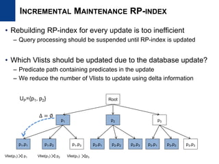
INCREMENTAL MAINTENANCE RP-INDEX
• Rebuilding RP-index for every update is too inefficient
– Query processing should be suspended until RP-index is updated
• Which Vlists should be updated due to the database update?
– Predicate path containing predicates in the update
– We reduce the number of Vlists to update using delta information
Root
p1 p2 p3
p1,p1 p1,p2 p1,p3 p2,p1 p2,p2 p2,p3 p3,p1 p3,p2 p3,p3
Δ = ∅
UP={p1, p2}
Vlist(p1) p1 Vlist(p1) p2 Vlist(p1) p3
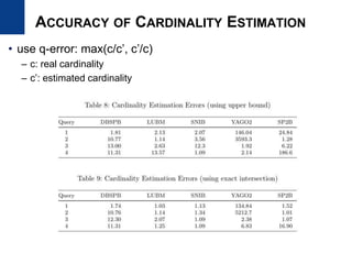
ACCURACY OF CARDINALITY ESTIMATION
• use q-error: max(c/c’, c’/c)
– c: real cardinality
– c’: estimated cardinality
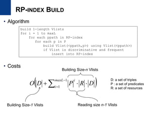
RP-INDEX BUILD
• Algorithm
• Costs
 



1
1
maxL
i
i
DRPDO
build 1-length Vlists
for i = 1 to maxL
for each ppath in RP-index
for each p in P
build Vlist(<ppath,p>) using Vlist(<ppath>)
if Vlist is discriminative and frequent
insert into RP-index
Building Size-1 Vlists Reading size n-1 Vlists
Building Size-n Vlists
D: a set of triples
P : a set of predicates
R: a set of resources
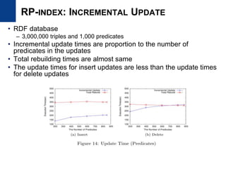
RP-INDEX: INCREMENTAL UPDATE
• RDF database
– 3,000,000 triples and 1,000 predicates
• Incremental update times are proportion to the number of
predicates in the updates
• Total rebuilding times are almost same
• The update times for insert updates are less than the update times
for delete updates
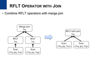
RFLT OPERATOR WITH JOIN
• Combine RFLT operators with merge join
Scan
<?v1, p1, ?v2>
RFLT
?v1
Merge Join
?v1
Scan
<?v1, p2, ?v3>
RFLT
?v1
Scan
<?v1, p1, ?v2>
RFLT with Join
?v1
Scan
<?v1, p2, ?v3>
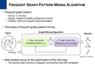
FREQUENT GRAPH PATTERN MINING ALGORITHM
• Frequent graph pattern
– 𝑆𝑢𝑝 𝑔 ≥ 𝑚𝑖𝑛𝑆𝑢𝑝
– Sup(g): support of graph g (frequency count)
– minSup: minimum support (input parameter)
• Two steps of frequent graph pattern mining
• Most studies focus on the optimization of the first step
– The second step involves a subgraph isomorphism test (NP-complete)
2nd step: check the
frequency of g, Sup(g)
1st step: generate
candidate pattern, g
Input
minSup
Graph Mining Algorithm
Results
𝑆𝑢𝑝 𝑔 ≥ 𝑚𝑖𝑛𝑆𝑢𝑝
OVERVIEW OF GSPAN
• X.Yan and J. Han, gSpan: Graph-based substructure pattern
mining, ICDM, 2002
• Popular algorithm for graph pattern mining
• Graph-transaction setting
– A set of relatively small graphs
• Depth-first style pattern generation
• Use DFS code
– To represent graph patterns
– To reduce redundant pattern generation
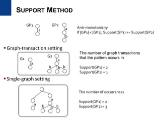
SUPPORT METHOD
Graph-transaction setting
Single-graph setting
a a
b
GP1 GP2
Anti-monotonicity
If |GP1| < |GP2|, Support(GP1) >= Support(GP2)
a
G2
G1 a
b b
The number of graph transactions
that the pattern occurs in
Support(GP1) = 2
Support(GP2) = 1
a
The number of occurrences
Support(GP1) = 2
Support(GP2) = 3
b
a
b bb
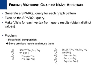
FINDING MATCHING GRAPHS: NAÏVE APPROACH
• Generate a SPARQL query for each graph pattern
• Execute the SPARQL query
• Make Vlists for each vertex from query results (obtain distinct
values)
• Problem
– Redundant computation
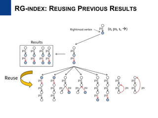
Store previous results and reuse them
p1
p1
p1 SELECT ?v1, ?v2, ?v3, ?v4
WHERE {
?v1 <p1> ?v2.
?v2 <p1> ?v3.
?v3 <p1> ?v4. }
p1
p1
SELECT ?v1, ?v2, ?v3
WHERE {
?v1 <p1> ?v2.
?v2 <p1> ?v3.}
RG-INDEX: REUSING PREVIOUS RESULTS
p1
p1
p1
p1
p1
p2
p1
p1
p1
p1
p1
p1
p1
p1
p2 p1
p1
p2
p2
p1
p1
p1p1
p1
p1p1
p1
(0, p1, 1, )Rightmost vertex
Results
p1
p1
p1
p1
p1
p1
p1
p1
Reuse
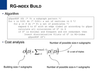
RG-INDEX BUILD
• Algorithm
• Cost analysis
gSpanRDF (G) /* V: a subgraph pattern */
for v in G(V) do /* G(V): a set of vertices in G */
for p in P do /* P: a set of predicates */
expand G to G’ with an edge (label p) according to gSpan
calculate all occurrences of G’ in D
if G’ is minimal and frequent and not redundant then
Insert discriminative Vlists of G’ in RG-index
gSpanRDF (G’)
 



1
1
maxL
i
i
DDDO
Building size-1 subgraphs Number of possible size-n-1 subgraphs
D: a set of triples
Number of possible size-n subgraphs
Clustered Property
Table
Sorted Triple Storage
Reducing Intermediate
Results
Method
Reducing joins using
materialized views
Store triples as sorted and use
merge joins
Build dynamic filters for join
variables
Pros
Reduce the number of joins •Efficient retrieval of matching
triples
•Fast merge join
Reduce redundant intermediate
results
Cons
•Need user’s clustering
decision
•Incur null and multi-values
which are hard to process
•Storage overhead
•Do not handle redundant
intermediate results
Do not exploit structural
information of RDF graphs
System
Jena
[Carroll et al., WWW 2004]
Oracle
[Chong et al., VLDB 2005]
SW-store
[Abadi et al., VLDB 2007]
RDF-3X
[Neumann and Weikum, VLDB 2008]
U-SIP
[Neumann and Weikum, SIGMOD’09]
EXISTING RELATIONAL RDF STORE
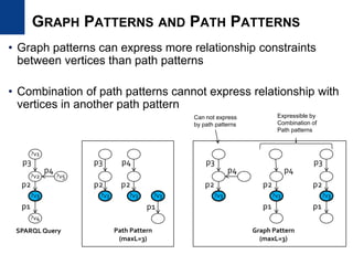
• Graph patterns can express more relationship constraints
between vertices than path patterns
• Combination of path patterns cannot express relationship with
vertices in another path pattern
?v3
?v4
?v2 ?v5
?v1
p3
p2
p4
p1
SPARQL Query
?v3
Path Pattern
(maxL=3)
Graph Pattern
(maxL=3)
p3
p2
p4
p2
p1
?v3 ?v3 ?v3
p3
p2
p4
?v3
p2
p4
p1
?v3
p3
p2
p1
Expressible by
Combination of
Path patterns
Can not express
by path patterns
GRAPH PATTERNS AND PATH PATTERNS
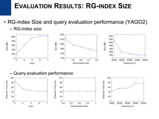
• RG-index Size and query evaluation performance (YAGO2)
– RG-index size
– Query evaluation performance
EVALUATION RESULTS: RG-INDEX SIZE
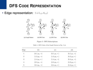
DFS CODE REPRESENTATION
• Edge representation:
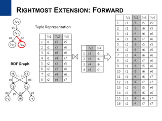
RIGHTMOST EXTENSION: FORWARD
?v2
?v1
p1
r3
r1
p1
r4
r5
r2
p1
p2 p2
RDF Graph
r6
p2
r7
p1
p1
p2
?v3 ?v4
p2 p2
Tuple Representation
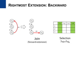
RIGHTMOST EXTENSION: BACKWARD
?v2
?v1
p1
?v3
p2
p2 ?v2
?v1
p1
?v3
p2
p2
?v4
Selection
?v1=?v4
Join
(forward extension)
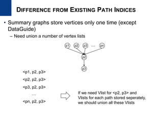
DIFFERENCE FROM EXISTING PATH INDICES
• Summary graphs store vertices only one time (except
DataGuide)
– Need union a number of vertex lists
<p1, p2, p3>
<p2, p2, p3>
<p3, p2, p3>
<pn, p2, p3>
… If we need Vlist for <p2, p3> and
Vlists for each path stored seperately,
we should union all these Vlists
p1
p2
p3
p2 p3 pn…

SPARQL and RDF query optimization

  • 1.
    SPARQL Query ProcessingTechniques using Structural Information of RDF Graphs in Relational RDF Store Seoul National University Internet Database Lab. Kisung Kim 2013. 11. 22 Ph.D Defense Presentation
  • 2.
    OUTLINE • Introduction – Motivation –Existing Approaches – Contributions • R3F: RDF Triple Filtering for SPARQL Query Processing • RP-Index: RDF Path index for Triple Filtering • RG-index: RDF Graph index for Triple Filtering • Conclusion & Future Work 2/39
  • 3.
    INTRODUCTION (1/8) RDF ISBIG GRAPH DATA • RDF (Resource Description Framework) – W3C recommendation in 1998 – General and flexible data model for sharing data via Web – Schema-less and graph-structure data model • Query processing over large-scale RDF graphs becomes more challenging Linking Open Data cloud diagram, by Richard Cyganiak and Anja Jentzsch. http://lod-cloud.net/ September, 2011 May, 2007 12 data sources 3/39
  • 4.
    • RDF – Aset of RDF triples (<Subject, Predicate, Object>) – Edge-labeled directed graph • SPARQL – Standard query language for RDF (W3C recommendation in 2008) – SELECT-FROM-WHERE form – Sub-graph pattern matching SPARQL Query INTRODUCTION (2/8) DATA MODEL OF RDF AND SPARQL RDFTriples <v1, p1, v2> <v2, p2, v4> <v3, p1, v2> <v2, p2, v5> v2 v4 v1 RDF Graph ?v1 ?v2 ?v3 SPARQL Query Graph SELECT * WHERE { <?v1, p1, ?v2> <?v2, p2, ?v3> } v3 v5 ?v1 ?v2 ?v3 v1 v2 v4 v1 v2 v5 v3 v2 v4 v3 v2 v5 Results Ex) <paper1, publicationType, ‘Survey Paper’> paper1 Survey Paper publicationType p1 p1 p2 p2 p1 p2 4/39
  • 5.
    Relational RDF StoreGraph RDF Store Storage Relational table Adjacent list Mainly In-memory Query Processing Relational operator Join and scan Sub-graph isomorphism algorithm System Jena [WWW2004] , Sesame [ISWC2002], Oracle [VLDB2005], SW-store [VLDBJ2009], RDF-3X [VLDBJ2010] GRIN [AAAI2007], Dogma [ISWC2009], PIG [SemData2010], gStore [VLDBJ2013] Pros Batch processing using Join operator Large-scale RDF processing [VLDB2012] Reduce search space of the graph traversal using the graph structure Cons Not using the graph structure Not scalable Inappropriate for large-scale processing INTRODUCTION (3/8) TWO TYPES OF RDF STORES 5/39
  • 6.
    • Most RDFstores use the relational model – Store RDF triples in relational tables (triple table) – Processing SPARQL queries using scan and join operators • Challenges of relational RDF stores – Involves many join operators – SPARQL query with N triple patterns requires N-1 joins • We will focus on the relational RDF stores INTRODUCTION (4/8) RELATIONAL RDF STORE Scan p1 Scan p2 Join1 Scan p3 Join2 SPARQL Graph S P O TripleTable Too many self-join Simple and General <?v1, p1, ?v2> <?v2, p2, ?v3> …. <?vn, pn, ?vn+1> Scan pn Joinn-1 …. 6/39
  • 7.
    • Storage approaches –Clustered property table – Jena [WWW2004] , Sesame [ISWC2002], Oracle [VLDB2005] – Cluster properties which are accessed together frequently – Sorted triple tables (multiple indexing) – SW-store [VLDBJ2009], RDF-3X [VLDBJ2010] – Store triples as sorted in a column-oriented store or clustered B+ trees ID Name age gender Clustered PropertyTable S P O SortedTripleTable S S P O P S P O O INTRODUCTION (5/8) EXISTING RELATIONAL RDF STORE Reduce joins Limited flexibility, Cluster decision Null value, Multi value Fast retrieval of matching triples Fast merge join Storage overhead, update 7/39
  • 8.
    • Handling intermediateresults approaches – Finding optimal plan – Static and traditional approach – Propose RDF-specific histograms – RDF-3X [VLDBJ2010], Characteristics set [ICDE2011], ARQ [WWW2008] – Dynamic filtering method – Build dynamic filters and use subsequent operators – U-SIP [SIGMOD2009] • Existing methods do not exploit graph structure of RDF graphs Scan p1 Scan p2 Merge Join Scan p3 Hash Join Next Information Domain Filter Scan p1 Scan p2 Merge Join Scan p3 Hash Join Finding Optimal Plan (static) Dynamic Filtering Method INTRODUCTION (6/8) EXISTING RELATIONAL RDF STORE 8/39
  • 9.
    • Reduce intermediateresults using structure of RDF graphs in relational RDF stores • We propose RDF triple filtering method – Filter irrelevant triples in advance – Reduce intermediate results using graph structure INTRODUCTION (7/8) OUR APPROACH: RDF TRIPLE FILTERING v3 v4 v2 v5 v1 v8 v9 v7 v10 v6 v11 v14 v15 v13 v12 p3 p2 p1 p4 p3 p2 p1 p2 p4 p3 p2 p1 RDF Graph Scan p1 Scan p2 Join1 Scan p3 Join2 Scan p4 Join3 ?v2 ?v3 ?v4 ?v5 v2 v3 v3 v4 v7 v8 v8 v9 v13 v14 v14 v15 Redundant Intermediate Results ?v3 ?v4 ?v2 ?v5 ?v1 p3 p2 p4 p1 SPARQL Query 9/39
  • 10.
    • RDF triplefiltering framework (R3F) – Filtering out irrelevant triples in advance – Reducing redundant intermediate results during SPARQL processing – Incorporate triple filtering method in relational RDF processing framework – Deal with whole query processing steps • We propose two indices for R3F – RP-index (RDF Path index) – Path-based index designed for efficient RDF triple filtering – Deal with several issues: size problem, building and maintenance – RG-index (RDF Graph index) to overcome the limitation of RP-index – Use sub-graph pattern mining algorithm – Propose efficient sub-graph pattern mining for RDF graphs INTRODUCTION (8/8) CONTRIBUTIONS: SUMMARY 10/39
  • 11.
    OUTLINE • Introduction • R3F:RDF Triple Filtering for SPARQL Query Processing – Motivation – Overview of R3F – Three components of R3F • RP-Index: RDF Path Index for R3F • RG-index: RDF Graph index for Triple Filtering • Conclusion & Future Work 11/39
  • 12.
    • Goal – Providegeneral framework for RDF triple filtering – Use structural information of RDF graphs in relational RDF stores – Incorporate triple filtering feature in existing relational RDF stores • Three components of R3F – Materialized filter data built using structural information – Relation filtering operator – Cardinality estimation method of the filtering operator • We assume that the retrieved triples from scan operators are sorted by subject or object column – Triples are stored as sorted in many RDF stores for efficient triple retrieval and using merge joins R3F (1/6) MOTIVATION 12/39
  • 13.
    Query Execution Engine Query Optimizer SPARQLQuery Plan Statistical Information Triple Storage Triples Results RDF Store Filter Data RP-index, RG-index RFLT Operator Cardinality Estimation of RFLT Operator Loader Updater RDF Data (RDF/XML, N3, …) Triple Table Index, HistogramIndex Updater R3F (2/6) SYSTEM OVERVIEW Filter Data 13/39
  • 14.
    • Answer verticesshould satisfy some structural conditions • Provide lists of vertices which satisfy a specific structural conditions • Candidate vertex (CV) for a query vertex – Superset of final results – Define candidate vertex set using several query structure • Vertex lists (Vlist) provide CVs as sorted lists ?v3 ?v4 ?v2 ?v5 ?v1 p3 p2 p4 p1 SPARQL Query v3 v4 v2 v5 v1 v8 v9 v7 v10 v6 v11 v14 v15 v13 v12 p3 p2 p1 p4 p3 p2 p1 p2 p4 p3 p2 p1 Answers for ‘?v3’? should have two incoming path patterns <p3, p2> and <p4, p2> Vlist (<p3, p2>)=v3, v8, v14 Vlist (<p4, p2>)=v3, v8 R3F (3/6) FILTER DATA RDF Graph 14/39
  • 15.
    • Perform triplefiltering for scan operators • Filter triples whose filtering keys are not in CV sets • Filtering by N-way merge process • Input triples are sorted in many RDF stores • Vlists are also stored as sorted • Need sequential I/O (reading Vlists) and merge process Scan <?v3, p1, ?v4> RFLT ?v3v3 v8 v3 v4 v8 v9 v14 v15 ?v3 ?v4 ?v2 ?v5 ?v1 p3 p2 p4 p1 SPARQL Query CV for ?v3 v3 v4 v8 v9 R3F (4/6) FILTERING OPERATOR: RFLT Filtering Key Input triples Output triples 15/39
  • 16.
    • Output cardinalityestimation is essential for the cost-based optimizer (CBO) • Cardinality estimation of RFLT operator – Assume the uniform distribution for filtering key values – Use the set intersection estimation method: e.g. • CBO determines based-on estimated cardinality – Whether to apply an RFLT operator for a scan operator – Which Vlists to be used Scan <?v3, p1, ?v4> RFLT ?v3 v3 v8 Vlist for ?v3 R3F (5/6) QUERY OPTIMIZATION v3 v4 v8 v9 v14 v15 v3 v4 v8 v9 Input triples Output triples   Scan FK FKvlist RFLT Vvlist     V : a set of Vlists for RFLT FK : a set of filtering key values Intersection estimation From statistical information 23 3 2 |}14,8,3{| }14,8,3{}8,3{ ||   Scan vvv vvvvv RFLT  16/39
  • 17.
    R3F (6/6) SUMMARY OFR3F RP-index RG-index Filter data as sorted list Query Optimizer SPARQL Query Optimized Plan with RFLT operator Query Executor RFLT Operator Results Statistical information R3F 17/39
  • 18.
    OUTLINE • Introduction • R3F:RDF Triple Filtering • RP-Index: RDF Path Index for R3F – Design of RP-Index – Size Problem – Experimental Results • RG-index: RDF Graph index for Triple Filtering • Conclusion & Future Work 18/39
  • 19.
    • Motivation – Designan index to provide vertex lists having a specific path pattern – Efficient and updatable index • Related work: path-based index – DataGuide [VLDB1997], 1-index [ICDT1999], A(k)-index [ICDE2002], D(k)-index [SIGMOD2003], M(k)-index [ICDE2004] – Provide a concise summary of the original data for query processing – Handle size problem by store every vertex one time in the index • Our goal is to provide filter data efficiently – Vertices can be stored several times and stored as sorted – We deal with the size problem differently RP-INDEX (1/7) MOTIVATION AND RELATED WORK 19/39
  • 20.
    • Provide CVsets using predicate path patterns • Predicate path pattern – A sequence of predicate: e.g. <p1, p2, p3> • Definition: RP-index (RDF Database D, maxL) – A set of <ppath, Vlist(ppath)>, where ppath exists in D and |ppath| ≤ maxL • We also index reverse predicates (outgoing edges) v3 v4 v2 v5 v1 v8 v9 v7 v10 v6 v11 v14 v15 v13 v12 p3 p2 p1 p4 p3 p2 p1 p2 p4 p3 p2 p1 ?v3 ?v4 ?v2 ?v5 ?v1 p3 p2 p4 p1 SPARQL Query CV for ?v3 = Vlist(<p3, p2>) ∩ Vlist(p4, p2) = {v3, v8} RP-INDEX (2/7) DESIGN OF RP-INDEX ?v1 ?v2 ?v3 p1 p2 ?v4 p3 RDF Graph Vlist (<p1>) = v4 Vlist (<p2>) = v3 Vlist (<p3>) = v2 Vlist (<p4>) = v2 Vlist (<p1R>) = v3 Vlist (<p2R>) = v2 Vlist (<p3R>) = v1 Vlist (<p4R>) = v5 Vlist (<p2, p1>) = v4 Vlist (<p3, p2>) = v3 Vlist (<p4, p2>) = v3 Vlist (<p1R,p2R>) = v2 Vlist (<p2R,p3R>) = v1 Vlist (<p2R,p4R>) = v5 Vlist(<p2,p2R>)=v11 Vlist(<p3,p4R>)=v5 RP–index (D, 2) with reverse predicate 20/39
  • 21.
    • Exponential numberof predicate paths , where |P| is the number of predicates • Solution – Choose effective predicate path for filtering • Two criteria for choosing predicate paths – Discriminative predicate path: use a replaceable predicate path – Frequent predicate path: infrequent Vlists are rarely used )||( 1 maxL i i PO r1 r2 r3 r4 r5 r6 r7 r2 r3 r4 r6 r7 Vlist(<p2, p3>) Vlist(<p1,p2,p3>) |Vlist(<p2,p3>)| / |Vlist(<p1,p2,p3>)| = 5/7 = 0.71 ∩ RP-INDEX (3/7) SIZE PROBLEM OF RP-INDEX If discriminative ratio is 0.7, then Vlist(<p1, p2, p3>) is not stored If minimum frequency is 7, then Vlist(<p1, p2, p3>) is not stored r2 r3 r4 r6 r7 Vlist(<p1,p2,p3>) Discriminative Predicate Path Frequent Predicate Path 21/39
  • 22.
    • Build Vlist(ppath)using Vlist of the longest proper prefix of ppath – Reduce redundant computation • Incremental update – Predicate path containing predicates in the update – We reduce the number of Vlists to update using delta information RP-INDEX (4/7) BUILDING AND MAINTENANCE  3,2,1 pppVlist 2,1 ppVlistJoin with and P3  Root p1 p2 p3 p1,p1 p1,p2 p1,p3 p2,p1 p2,p2 p2,p3 p3,p1 p3,p2 p3,p3 UP={p1, p2} Vlist(p1) p1 Vlist(p1) p2 Vlist(p1) p3 22/39
  • 23.
    • Experimental environment –We implemented R3F and RP-index on the top of an open source RDF store, RDF-3X (0.3.6)* – IBM machine having 8 Intel Xeon 3.0 GHz cores, 16 GB memory • Datasets – LUBM (Leihigh University Benchmark) : university domain – SP2B (SPARQL Performance Benchmark) : DBLP scenario – DBSPB (DBpedia SPARQL Benchmark) : DBpedia Predicates Triples RDF-3X Size (GB) LUBM 18 1,335 M 77 SP2B 77 1,399 M 123 DBSPB 39,675 183 M 25 Dataset Statistics RP-INDEX (5/7) EXPERIMENTAL RESULTS: SETTING Synthetic dataset Real-world characteristics * https://code.google.com/p/rdf3x/ 23/39
  • 24.
    • We builtthree RP-indices (maxL=3) • RP-index is much smaller than database Setting LUBM SP2B DBSPB 1 0.307 2.05 2.85 2 19.12 87.99 N/A 3 1.39 21.97 6.52 Setting Discriminative Ratio Frequency Function Reverse Predicate 1 1 0 not included 2 1 0 included 3 0.7 (l-1/maxL)2 X n included Parameter Settings RP-index Size (GB) RP-INDEX (6/7) EXPERIMENTAL RESULTS: RP-INDEX SIZE LUBM SP2B DBPSB 77 123 25 Database Size (GB) 24/39
  • 25.
    • For mostqueries, R3F using RP-index reduces the execution times • Including reverse predicate is more effective for triple filtering • Indexing only discriminative and frequent predicate path does not degrade query performance much RP-INDEX (7/7) EXPERIMENTAL RESULTS (a) LUBM (b) SP2B (C) DBSPB 25/39
  • 26.
    OUTLINE • Introduction • R3F:RDF Triple Filtering using RG-index • RP-Index: RDF Path Index for R3F • RG-index: RDF Graph index for Triple Filtering – Motivation – Design of RG-index – Building RG-index – Evaluaion Results • Conclusion & Future Work 26/39
  • 27.
    • Limited filteringpower of RP-index – Use only path information for graph-structural RDF data • Need to index graph structures RP-index cannot filter out this result ?v3 ?v4 ?v2 ?v5 ?v1 p3 p2 p4 p1 SPARQL Query v3 v4 v2 v5 v1 v8 v9 v7 v10 v6 v11 v14 v15 v13 v12 p3 p2 p1 p4 p3 p2 p1 p2 p4 p3 p2 p1 RG-INDEX (1/11) MOTIVATION RDF Graph 27/39
  • 28.
    • Graph index –Graph-transactional setting (many small graphs) – GraphGrep [PODS2002], gIndex [SIGMOD2004], C-tree [ICDE2006], QuckSI [VLDB2008], Tale [ICDE2008] – A single large graph – GraphQL [SIGMOD2008], GADDI [EDBT2009], SPath [VLDB2010] – For reducing the search space of the graph traversal – Non-trivial to apply to relational RDF stores • Subgraph pattern mining – Graph-transactional setting – gSpan [ICDM2002], Gaston [KDD2004] – A single large graph – HSIGRAM, VSIGRAM [JDMKD2005] – Not scalable for large RDF graphs – We need to adapt existing algorithm for RDF graphs RG-INDEX (2/11) RELATED WORK 28/39
  • 29.
    • Graph pattern –A graph which all vertices are variables and all predicates are bound • Definition: RG-index (D, maxL) – A set of <gp, VS(gp)>, where gp is a graph pattern in D and |gp| ≤ maxL, VS(gp) is the set of Vlists for vertices in gp Graph Pattern ?v1 ?v2Size: 1 ?v1 ?v2 Size: 2 Size: maxL ?v3 VlistsRG-index Vlist(gp1, ?v1) RG-INDEX (3/11) DESIGN OF RG-INDEX p1 p1 p2 gp1 gp2 Vlist(gp1, ?v2) Vlist(gp2, ?v1) Vlist(gp2, ?v2) Vlist(gp2, ?v3) 29/39
  • 30.
    • Use subgraphmining due to the size problem of RG-index – Indexing only frequent subgraph patterns  Frequent subgraph mining • Adapt gSpan [Yan and Han, ICDM ’02] algorithm for RDF graphs • gSpan – Transactional setting – Depth-first pattern growth approach – Use anti-monocity property of support – Use DFS encoding and edge extension to prevent duplicate pattern generation RG-INDEX (4/11) BUILDING RG-INDEX USING SUBGRAPH MINING size-2 size-1 size-maxL Edge extension pruning infrequent or duplicate pattern 30/39
  • 31.
    • Pattern representation –Use DFS code and extend it to directed edge-label graph [SIGKDD2003] • Support definition – Should satisfy anti-monotonicity property for efficient mining – Most mining algorithm use MIS (maximum independent set) approach, which is NP-hard for the single large setting – We use support definition in [Bringmann and Nijssen, PAKDD ‘08] as minimum matching vertex number – Very efficient to compute and upper-bound of MIS approaches (mining more patterns) |)),((|min)sup( vGVlistG Vv RG-INDEX (5/11) ADAPTING GSPAN FOR RDF GRAPHS 31/39
  • 32.
    • Redundant subgraphpatterns – Graph patterns with same Vlists – Graphs having non-trivial automorphisms • Compute occurrences of graph pattern – Exploit depth-first style pattern generation similarly to VSIGRAM [JDMKD2005] – Store all occurrences of a pattern to compute child patterns – Store occurrences from root to a leaf (depth-first approach) – We propose efficient occurrence computation method RG-INDEX (6/11) ADAPTING GSPAN FOR RDF GRAPHS Redundant patterns 32/39
  • 33.
    • Data sets –YAGO2: Yet Another Great Ontology 2 • Index build RG-INDEX (7/11) EVALUATION RESULTS Predicates Triples RDF-3X Size (GB) LUBM 18 1,335 M 77 YAGO2 93 37 M 9 SP2B 77 1,399 M 123 Dataset Statistics Setting YAGO2 LUBM SP2B RP-index 341 MB 1.4 GB 1.3 GB RP-index (R) 2.3 G 1.7 G 3.1 GB RG-index 880 MB 1.1 G 1.3 GB Setting Discriminative Ratio Frequency Function Reverse Predicate RP-index 1 0 not included RP-index (R) 0.7 (l-1/maxL)2 X n included RG-index 0.7 (l-1/maxL)2 X n N/A Parameter Settings Index Size (GB) 33/39
  • 34.
    • Query sets –Extract graph patterns from each data set – Use these patterns as test queries – Divide the queries into four groups according to their evaluation times in RDF-3X RG-INDEX (8/11) EVALUATION RESULTS: QUERY PERFORMANCE Test Query Groups Group Execution Times (ms) A 0~10 B 10~100 C 100~1000 D 1000~ Total avg. YAGO2 824 143 41 19 1,027 LUBM 0 7 14 45 67 SP2B 161 210 187 7 565 34/39
  • 35.
    Group A BC D Total RDF-3X 2.76 29.02 244.62 1383.42 108.65 RP-index 2.38 (13%) 25.2 (13%) 182.72 (25%) 555.42 (59%) 76.08 (30%) RP-index (reverse) 2.39 (13%) 25.2 (13%) 153.92 (37%) 127 (91%) 61.06 (43.8%) RG-index 2.33 (15%) 16.39 (43%) 122.8 (49%) 106.85 (92%) 44.34 (59.19%) RG-INDEX (9/11) EVALUATION RESULTS: QUERY PERFORMANCE Group A B C D Total RDF-3X N/A 59 444.6 2158.6 1548.8 RP-index N/A 58 (1%) 441. 6 (0.6%) 2126.9 (0.1%) 1526.8 (1%) RP-index (reverse) N/A 50 (15%) 420 (5%) 1274.1 (40%) 946.4 (38%) RG-index N/A 50 (15%) 406 (8%) 1250.2 (42%) 929.7 (40%) Group A B C D Total RDF-3X 3.53 34.18 240.43 16671.261 325.62 RP-index 2.75 (22%) 11.83 (65%) 94.73 (60%) 9194.21 (44%) 177.73 (45%) RP-index (reverse) 3.00 (15%) 17.82 (47%) 79.78 (66%) 4747.26 (71%) 95.90 (70%) RG-index 2.32 (34%) 8.65 (74%) 27.60 (88%) 581.36 (96%) 14.92 (95%) SP2B (ms) LUBM (ms) YAGO2 (ms) 35/39
  • 36.
    • RG-index ismore effective for YAGO2 and SP2B than LUBM • RG-index is more effective for queries with longer evaluation times • RG-index is more effective than RP-index and RP-index with reverse predicate – RG-index is smaller than RP-index with reverse predicate RG-INDEX (10/11) EVALUATION RESULTS: QUERY PERFORMANCE 36/39
  • 37.
    Frequency=1000 Frequency=2000 Frequency=4000 BuildTime 5776.25 secs 3290.53 secs 1381.61 secs Query Time 171.25 msecs 169.46 msec 187.34 msecs Not including reverse predicates including reverse predicates (frequency = 1000) including reverse predicates (frequency = 2000) including reverse predicates (frequency = 4000) Build Time 93.33 secs 449.33 secs 299.79 secs 164.88 secs Query Time 368.19 msecs 254.0 msecs 254.01 msecs 258.3 msecs RDF-3X Loading Time 4264 secs Query Time 409.4 msecs RP-index (maxL=5, discriminative ratio = 0.8) RG-index (maxL=5 , discriminative ratio = 0.8) Include loading triples, Building triple indices, computing statistics RG-INDEX (11/11) EVALUATION RESULTS: INDEX BUILD TIME (YAGO2) 37/39 RDF-3X
  • 38.
    CONCLUSIONS • We proposeRDF triple filtering method for handling redundant intermediate results of SPARQL query processing (Chapter 4) – Provide a framework for filtering irrelevant triples • We propose RP-index which uses path information (Chapter 4) – Deal with size problem and maintenance issues • We propose RG-index which uses graph-structural information (Chapter 5) – Improve the filtering power of RP-index – Use frequent sub-graph mining algorithm for building RG-index 38/39
  • 39.
    FUTURE WORK • Indexingpatterns considering query workload – More effective triple filtering for current query workload • More accurate estimation of cardinality – We have assumed the uniform distribution – Very crucial for the query evaluation performance • Applying distributed environment – Handling intermediate results is more important in MapReduce – How to store and access the index 39/39
  • 40.
    PAPERS • R3F andRP-index – Kisung Kim, Bongki Moon, Hyoung-Joo Kim, RP-Filter: A Path-based Triple Filtering Method for Efficient SPARQL Query Processing, JIST (Joint International Semantic Technology) conference, 2011 – Kisung Kim, Bongki Moon, Hyoung-Joo Kim, R3F: RDF Triple Filtering Method for Efficient SPARQL Query Processing, Accepted, Online first published, World Wide Web Journal (Springer), 2013 • RG-index – Kisung Kim, Bongki Moon, Hyoung-Joo Kim, RG-index: an RDF Graph Index for Efficient SPARQL Query Processing Submitted to ESWA Expert Systems with Applications (Elsevier), under review
  • 41.
  • 42.
    RP-INDEX: TRIE OFPREDICATE PATHS • Search the Vlist of a given predicate path – Each node has a pointer to the Vlist of the corresponding predicate paths
  • 43.
    • Indexing pathpatterns other than incoming path • Redundant predicate path – We do not index predicate path pattern such as p, pR v3 v4 v2 v5 v1 p3 p2 p1 p4 RP-index (R, 2) Vlist (<p1>) = v4 Vlist (<p2>) = v3 Vlist (<p3>) = v2 Vlist (<p4>) = v2 Vlist (<p1R>) = v3 Vlist (<p2R>) = v2 Vlist (<p3R>) = v1 Vlist (<p4R>) = v5 P = {p1, p2, p3, p4} P = {p1, p2, p3, p4 p1R, p2R, p3R, p4R} p3R p2R p1R p4R Vlist (<p2, p1>) = v4 Vlist (<p3, p2>) = v3 Vlist (<p4, p2>) = v3 Vlist (<p1R,p2R>) = v2 Vlist (<p2R,p3R>) = v1 Vlist (<p2R,p4R>) = v5 REVERSE PREDICATE RP-index (D, 2) Vlist (<p1>) = v4, v9, v15 Vlist (<p2>) = v3, v8, v14 Vlist (<p3>) = v2, v7, v13 Vlist (<p4>) = v2, v8 Vlist (<p2, p1>) = v4, v9, v15 Vlist (<p3, p2>) = v3, v8, v14 Vlist (<p4, p2>) = v3, v8
  • 44.
    BUILDING RP-INDEX • BuildRP-index in the Breadth-First Search (BFS) manner • Vlists for (i + 1)-length predicate paths is built using Vlists for i- length predicate path Root p1 p2 p3 p1,p1 p1,p2 p1,p3 p2,p1 p2,p2 p2,p3 p3,p1 p3,p2 p3,p3 Vlist(p1) p1 Vlist(p1) p2 Vlist(p1) p3
  • 45.
    PARALLEL BUILDING OFRP-INDEX • Building each Vlists is independent • We can build multiple Vlists while reading triples once 1 Thread 2 Threads 4 Threads Build Time 503.43 secs 349 secs 238.84 Including reverse predicates (frequency = 1000)
  • 46.
    INCREMENTAL MAINTENANCE RP-INDEX •Rebuilding RP-index for every update is too inefficient – Query processing should be suspended until RP-index is updated • Which Vlists should be updated due to the database update? – Predicate path containing predicates in the update – We reduce the number of Vlists to update using delta information Root p1 p2 p3 p1,p1 p1,p2 p1,p3 p2,p1 p2,p2 p2,p3 p3,p1 p3,p2 p3,p3 Δ = ∅ UP={p1, p2} Vlist(p1) p1 Vlist(p1) p2 Vlist(p1) p3
  • 47.
    ACCURACY OF CARDINALITYESTIMATION • use q-error: max(c/c’, c’/c) – c: real cardinality – c’: estimated cardinality
  • 48.
    RP-INDEX BUILD • Algorithm •Costs      1 1 maxL i i DRPDO build 1-length Vlists for i = 1 to maxL for each ppath in RP-index for each p in P build Vlist(<ppath,p>) using Vlist(<ppath>) if Vlist is discriminative and frequent insert into RP-index Building Size-1 Vlists Reading size n-1 Vlists Building Size-n Vlists D: a set of triples P : a set of predicates R: a set of resources
  • 49.
    RP-INDEX: INCREMENTAL UPDATE •RDF database – 3,000,000 triples and 1,000 predicates • Incremental update times are proportion to the number of predicates in the updates • Total rebuilding times are almost same • The update times for insert updates are less than the update times for delete updates
  • 50.
    RFLT OPERATOR WITHJOIN • Combine RFLT operators with merge join Scan <?v1, p1, ?v2> RFLT ?v1 Merge Join ?v1 Scan <?v1, p2, ?v3> RFLT ?v1 Scan <?v1, p1, ?v2> RFLT with Join ?v1 Scan <?v1, p2, ?v3>
  • 51.
    FREQUENT GRAPH PATTERNMINING ALGORITHM • Frequent graph pattern – 𝑆𝑢𝑝 𝑔 ≥ 𝑚𝑖𝑛𝑆𝑢𝑝 – Sup(g): support of graph g (frequency count) – minSup: minimum support (input parameter) • Two steps of frequent graph pattern mining • Most studies focus on the optimization of the first step – The second step involves a subgraph isomorphism test (NP-complete) 2nd step: check the frequency of g, Sup(g) 1st step: generate candidate pattern, g Input minSup Graph Mining Algorithm Results 𝑆𝑢𝑝 𝑔 ≥ 𝑚𝑖𝑛𝑆𝑢𝑝
  • 52.
    OVERVIEW OF GSPAN •X.Yan and J. Han, gSpan: Graph-based substructure pattern mining, ICDM, 2002 • Popular algorithm for graph pattern mining • Graph-transaction setting – A set of relatively small graphs • Depth-first style pattern generation • Use DFS code – To represent graph patterns – To reduce redundant pattern generation
  • 53.
    SUPPORT METHOD Graph-transaction setting Single-graphsetting a a b GP1 GP2 Anti-monotonicity If |GP1| < |GP2|, Support(GP1) >= Support(GP2) a G2 G1 a b b The number of graph transactions that the pattern occurs in Support(GP1) = 2 Support(GP2) = 1 a The number of occurrences Support(GP1) = 2 Support(GP2) = 3 b a b bb
  • 54.
    FINDING MATCHING GRAPHS:NAÏVE APPROACH • Generate a SPARQL query for each graph pattern • Execute the SPARQL query • Make Vlists for each vertex from query results (obtain distinct values) • Problem – Redundant computation Store previous results and reuse them p1 p1 p1 SELECT ?v1, ?v2, ?v3, ?v4 WHERE { ?v1 <p1> ?v2. ?v2 <p1> ?v3. ?v3 <p1> ?v4. } p1 p1 SELECT ?v1, ?v2, ?v3 WHERE { ?v1 <p1> ?v2. ?v2 <p1> ?v3.}
  • 55.
    RG-INDEX: REUSING PREVIOUSRESULTS p1 p1 p1 p1 p1 p2 p1 p1 p1 p1 p1 p1 p1 p1 p2 p1 p1 p2 p2 p1 p1 p1p1 p1 p1p1 p1 (0, p1, 1, )Rightmost vertex Results p1 p1 p1 p1 p1 p1 p1 p1 Reuse
  • 56.
    RG-INDEX BUILD • Algorithm •Cost analysis gSpanRDF (G) /* V: a subgraph pattern */ for v in G(V) do /* G(V): a set of vertices in G */ for p in P do /* P: a set of predicates */ expand G to G’ with an edge (label p) according to gSpan calculate all occurrences of G’ in D if G’ is minimal and frequent and not redundant then Insert discriminative Vlists of G’ in RG-index gSpanRDF (G’)      1 1 maxL i i DDDO Building size-1 subgraphs Number of possible size-n-1 subgraphs D: a set of triples Number of possible size-n subgraphs
  • 57.
    Clustered Property Table Sorted TripleStorage Reducing Intermediate Results Method Reducing joins using materialized views Store triples as sorted and use merge joins Build dynamic filters for join variables Pros Reduce the number of joins •Efficient retrieval of matching triples •Fast merge join Reduce redundant intermediate results Cons •Need user’s clustering decision •Incur null and multi-values which are hard to process •Storage overhead •Do not handle redundant intermediate results Do not exploit structural information of RDF graphs System Jena [Carroll et al., WWW 2004] Oracle [Chong et al., VLDB 2005] SW-store [Abadi et al., VLDB 2007] RDF-3X [Neumann and Weikum, VLDB 2008] U-SIP [Neumann and Weikum, SIGMOD’09] EXISTING RELATIONAL RDF STORE
  • 58.
    • Graph patternscan express more relationship constraints between vertices than path patterns • Combination of path patterns cannot express relationship with vertices in another path pattern ?v3 ?v4 ?v2 ?v5 ?v1 p3 p2 p4 p1 SPARQL Query ?v3 Path Pattern (maxL=3) Graph Pattern (maxL=3) p3 p2 p4 p2 p1 ?v3 ?v3 ?v3 p3 p2 p4 ?v3 p2 p4 p1 ?v3 p3 p2 p1 Expressible by Combination of Path patterns Can not express by path patterns GRAPH PATTERNS AND PATH PATTERNS
  • 59.
    • RG-index Sizeand query evaluation performance (YAGO2) – RG-index size – Query evaluation performance EVALUATION RESULTS: RG-INDEX SIZE
  • 60.
    DFS CODE REPRESENTATION •Edge representation:
  • 61.
    RIGHTMOST EXTENSION: FORWARD ?v2 ?v1 p1 r3 r1 p1 r4 r5 r2 p1 p2p2 RDF Graph r6 p2 r7 p1 p1 p2 ?v3 ?v4 p2 p2 Tuple Representation
  • 62.
    RIGHTMOST EXTENSION: BACKWARD ?v2 ?v1 p1 ?v3 p2 p2?v2 ?v1 p1 ?v3 p2 p2 ?v4 Selection ?v1=?v4 Join (forward extension)
  • 63.
    DIFFERENCE FROM EXISTINGPATH INDICES • Summary graphs store vertices only one time (except DataGuide) – Need union a number of vertex lists <p1, p2, p3> <p2, p2, p3> <p3, p2, p3> <pn, p2, p3> … If we need Vlist for <p2, p3> and Vlists for each path stored seperately, we should union all these Vlists p1 p2 p3 p2 p3 pn…

Editor's Notes

  • #8 relational rdf store의 문제점 해결 방안
  • #10 우리는 relational rdf store에 graph index를 적용하는 방안으로 triple filtering을 제안한다.
  • #42 And that ends my talk Thank you for your attention.