Download as PDF, PPTX
![Lambda calculus [Church’36]
Formal system to study the defini-
tion of function
f (x) ∼ tx
x → f (x) ∼ λx.tx
(x → f (x))r ∼ (λx.tx ) r
(x → f (x))r = f (r ) ∼ (λx.tx ) r → tx [r /x]
t, r ::= x | λx.t | (t) r
(λx.t) r → t[r/x]
2 / 24](https://image.slidesharecdn.com/du-typage-vectoriel-slides-120329081738-phpapp01/75/Slides-used-during-my-thesis-defense-Du-typage-vectoriel-2-2048.jpg)
![Lambda calculus [Church’36] Type system [Church’40]
Formal system to study the defini- “a tractable syntactic framework
tion of function for classifying phrases according to
f (x) ∼ tx the kinds of values they compute”
x → f (x) ∼ λx.tx –[Pierce’02]
(x → f (x))r ∼ (λx.tx ) r
(x → f (x))r = f (r ) ∼ (λx.tx ) r → tx [r /x] λx.tx : T → R r:T
t, r ::= x | λx.t | (t) r (λx.tx ) r : R
(λx.t) r → t[r/x]
2 / 24](https://image.slidesharecdn.com/du-typage-vectoriel-slides-120329081738-phpapp01/75/Slides-used-during-my-thesis-defense-Du-typage-vectoriel-3-2048.jpg)
![Lambda calculus [Church’36] Type system [Church’40]
Formal system to study the defini- “a tractable syntactic framework
tion of function for classifying phrases according to
f (x) ∼ tx the kinds of values they compute”
x → f (x) ∼ λx.tx –[Pierce’02]
(x → f (x))r ∼ (λx.tx ) r
(x → f (x))r = f (r ) ∼ (λx.tx ) r → tx [r /x] λx.tx : T → R r:T
t, r ::= x | λx.t | (t) r (λx.tx ) r : R
(λx.t) r → t[r/x]
System F [Girard’71]
TS with a universal quantification
over types
λx.x : Int → Int
λx.x : Bool → Bool
...
λx.x : ∀X .X → X
2 / 24](https://image.slidesharecdn.com/du-typage-vectoriel-slides-120329081738-phpapp01/75/Slides-used-during-my-thesis-defense-Du-typage-vectoriel-4-2048.jpg)
![Lambda calculus [Church’36] Type system [Church’40]
Formal system to study the defini- “a tractable syntactic framework
tion of function for classifying phrases according to
f (x) ∼ tx the kinds of values they compute”
x → f (x) ∼ λx.tx –[Pierce’02]
(x → f (x))r ∼ (λx.tx ) r
(x → f (x))r = f (r ) ∼ (λx.tx ) r → tx [r /x] λx.tx : T → R r:T
t, r ::= x | λx.t | (t) r (λx.tx ) r : R
(λx.t) r → t[r/x]
System F [Girard’71] Curry-Howard correspondence
TS with a universal quantification Correspondence between type sys-
over types tems and logic
λx.x : Int → Int λx.tx : T → R r:T
λx.x : Bool → Bool (λx.tx ) r : R
...
T ⇒R T
λx.x : ∀X .X → X
R
2 / 24](https://image.slidesharecdn.com/du-typage-vectoriel-slides-120329081738-phpapp01/75/Slides-used-during-my-thesis-defense-Du-typage-vectoriel-5-2048.jpg)
![Lambda calculus [Church’36] Type system [Church’40]
Formal system to study the defini- “a tractable syntactic framework
tion of function for classifying phrases according to
f (x) ∼ tx the kinds of values they compute”
x → f (x) ∼ λx.tx –[Pierce’02]
(x → f (x))r ∼ (λx.tx ) r
(x → f (x))r = f (r ) ∼ (λx.tx ) r → tx [r /x] λx.tx : T → R r:T
t, r ::= x | λx.t | (t) r (λx.tx ) r : R
(λx.t) r → t[r/x]
System F [Girard’71] Curry-Howard correspondence
TS with a universal quantification Correspondence between type sys-
over types tems and logic
λx Int .x : Int → Int λx.tx : T → R r:T
λx Bool .x : Bool → Bool (λx.tx ) r : R
...
T ⇒R T
ΛX .λx X .x : ∀X .X → X
R
Church vs. Curry style whether the types are part of the terms or not
2 / 24](https://image.slidesharecdn.com/du-typage-vectoriel-slides-120329081738-phpapp01/75/Slides-used-during-my-thesis-defense-Du-typage-vectoriel-6-2048.jpg)
![To capture probabilistic/quantum/quantitative constructions:
algebraic extensions
t, r ::= x | λx.t | (t) r | t + r | α.t | 0 α ∈ (S, +, ×), a ring.
Two origins:
Differential λ-calculus [Ehrhard’03]: linearity à la Linear Logic
Removing the differential operator : Algebraic λ-calculus (λalg ) [Vaux’09]
Quantum computing: superposition of programs
Linearity as in algebra: Linear-algebraic λ-calculus (λlin ) [Arrighi,Dowek’08]
3 / 24](https://image.slidesharecdn.com/du-typage-vectoriel-slides-120329081738-phpapp01/75/Slides-used-during-my-thesis-defense-Du-typage-vectoriel-7-2048.jpg)
![To capture probabilistic/quantum/quantitative constructions:
algebraic extensions
t, r ::= x | λx.t | (t) r | t + r | α.t | 0 α ∈ (S, +, ×), a ring.
Two origins:
Differential λ-calculus [Ehrhard’03]: linearity à la Linear Logic
Removing the differential operator : Algebraic λ-calculus (λalg ) [Vaux’09]
Quantum computing: superposition of programs
Linearity as in algebra: Linear-algebraic λ-calculus (λlin ) [Arrighi,Dowek’08]
Beta reduction:
(λx.t) r → t[r/x]
“Algebraic” reductions:
α.t + β.t → (α + β).t,
α.β.t → (α × β).t,
(t) (r1 + r2 ) → (t) r1 + (t) r2 ,
(t1 + t2 ) r → (t1 ) r + (t2 ) r,
...
(oriented version of the axioms of
vectorial spaces)[Arrighi,Dowek’07]
3 / 24](https://image.slidesharecdn.com/du-typage-vectoriel-slides-120329081738-phpapp01/75/Slides-used-during-my-thesis-defense-Du-typage-vectoriel-8-2048.jpg)
![To capture probabilistic/quantum/quantitative constructions:
algebraic extensions
t, r ::= x | λx.t | (t) r | t + r | α.t | 0 α ∈ (S, +, ×), a ring.
Two origins:
Differential λ-calculus [Ehrhard’03]: linearity à la Linear Logic
Removing the differential operator : Algebraic λ-calculus (λalg ) [Vaux’09]
Quantum computing: superposition of programs
Linearity as in algebra: Linear-algebraic λ-calculus (λlin ) [Arrighi,Dowek’08]
Beta reduction:
(λx.t) r → t[r/x]
“Algebraic” reductions:
α.t + β.t → (α + β).t, Vectorial space of values
α.β.t → (α × β).t, B = {ti : ti var. or abs. }
(t) (r1 + r2 ) → (t) r1 + (t) r2 ,
(t1 + t2 ) r → (t1 ) r + (t2 ) r, Set of values ::= Span(B)
...
(oriented version of the axioms of
vectorial spaces)[Arrighi,Dowek’07]
3 / 24](https://image.slidesharecdn.com/du-typage-vectoriel-slides-120329081738-phpapp01/75/Slides-used-during-my-thesis-defense-Du-typage-vectoriel-9-2048.jpg)
![To capture probabilistic/quantum/quantitative constructions:
algebraic extensions
t, r ::= x | λx.t | (t) r | t + r | α.t | 0 α ∈ (S, +, ×), a ring.
λalg λlin
Origin Linear Logic Quantum computing
Evaluation strategy Call-by-name Call-by-base
Algebraic part Equalities Rewrite system
Contribution: CPS simulation [Díaz-Caro,Perdrix,Tasson,Valiron’10]
Beta reduction:
(λx.t) r → t[r/x]
“Algebraic” reductions:
α.t + β.t → (α + β).t, Vectorial space of values
α.β.t → (α × β).t, B = {ti : ti var. or abs. }
(t) (r1 + r2 ) → (t) r1 + (t) r2 ,
(t1 + t2 ) r → (t1 ) r + (t2 ) r, Set of values ::= Span(B)
...
(oriented version of the axioms of
vectorial spaces)[Arrighi,Dowek’07]
3 / 24](https://image.slidesharecdn.com/du-typage-vectoriel-slides-120329081738-phpapp01/75/Slides-used-during-my-thesis-defense-Du-typage-vectoriel-10-2048.jpg)
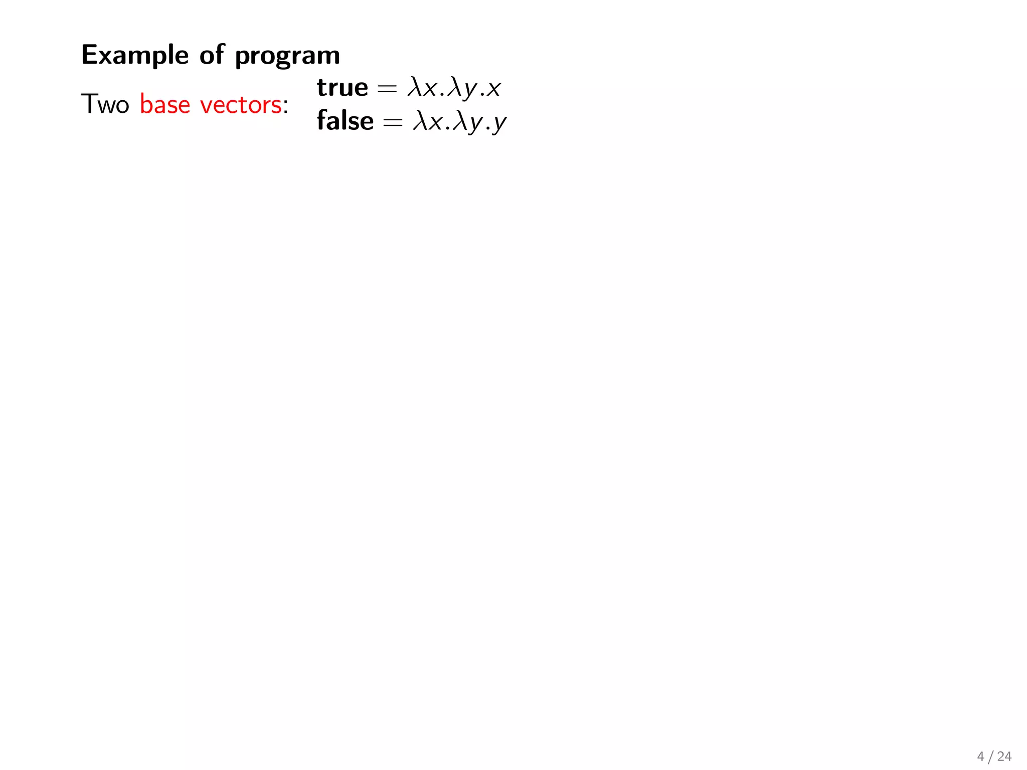
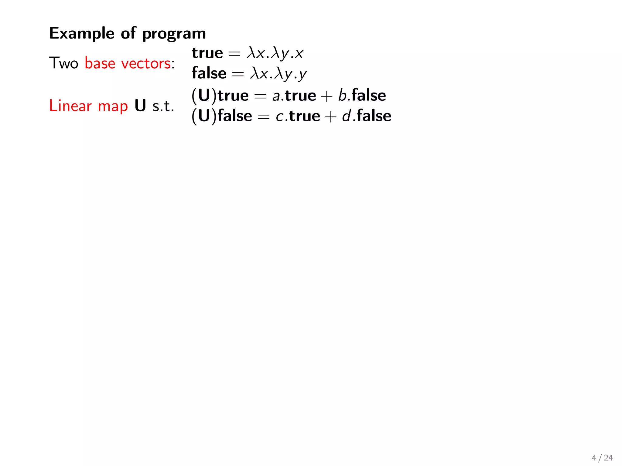
![Example of program
true = λx.λy .x
Two base vectors:
false = λx.λy .y
(U)true = a.true + b.false
Linear map U s.t.
(U)false = c.true + d .false
U := λx.{((x) [a.true + b.false]) [c.true + d .false]}
4 / 24](https://image.slidesharecdn.com/du-typage-vectoriel-slides-120329081738-phpapp01/75/Slides-used-during-my-thesis-defense-Du-typage-vectoriel-13-2048.jpg)
![Example of program
true = λx.λy .x
Two base vectors:
false = λx.λy .y
(U)true = a.true + b.false
Linear map U s.t.
(U)false = c.true + d .false
U := λx.{((x) [a.true + b.false]) [c.true + d .false]}
Aim:
To provide a type system capturing the “vectorial” structure of terms
. . . to check for properties of probabilistic processes
. . . to check for properties of quantum processes
. . . or whatever application needing the structure of the vector
in normal form
. . . understand what it means “linear combination of types”
. . . a Curry-Howard approach to defining
Fuzzy/Quantum/Probabilistic logics from
Fuzzy/Quantum/Probabilistic programming languages.
4 / 24](https://image.slidesharecdn.com/du-typage-vectoriel-slides-120329081738-phpapp01/75/Slides-used-during-my-thesis-defense-Du-typage-vectoriel-14-2048.jpg)
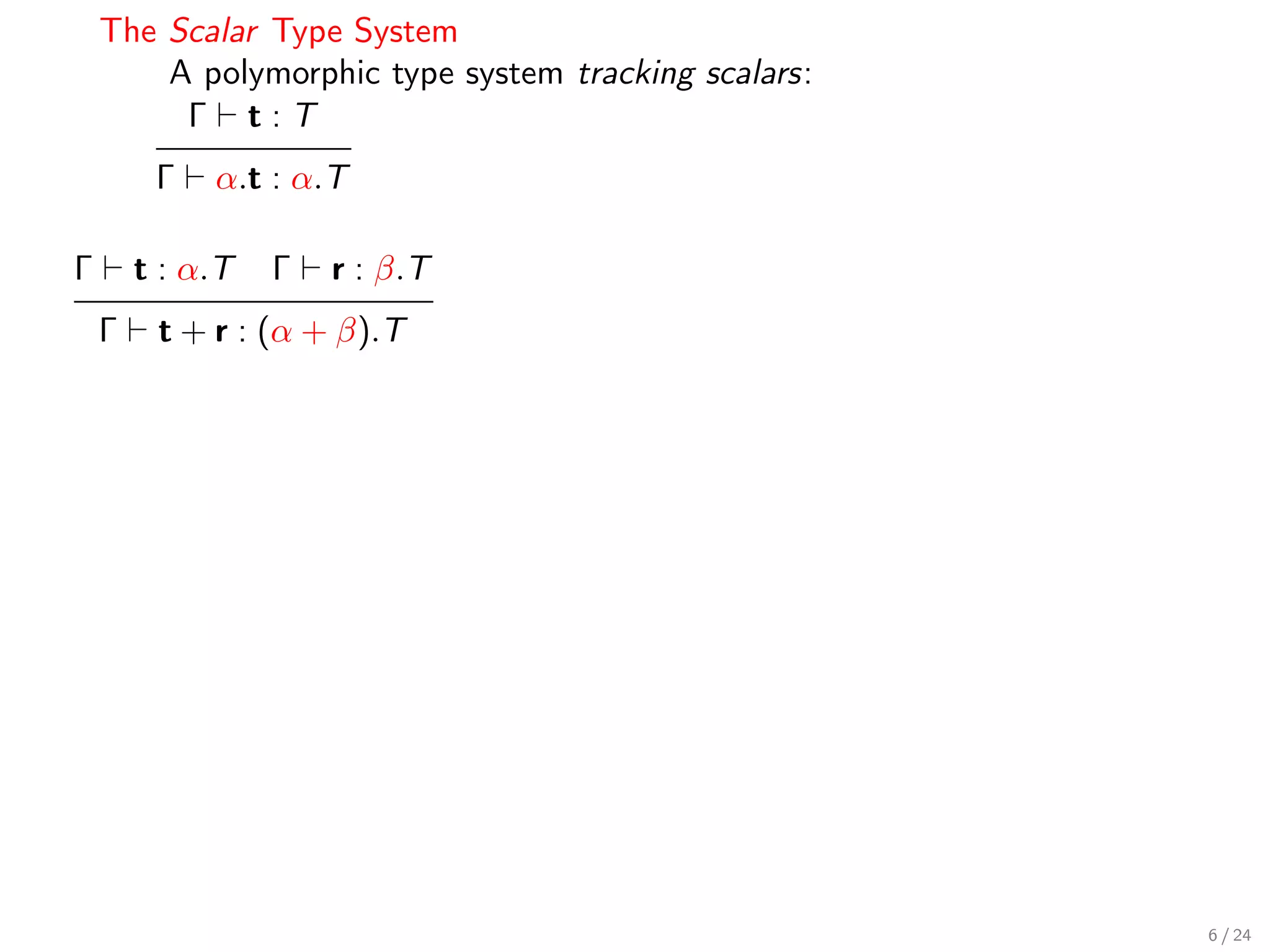
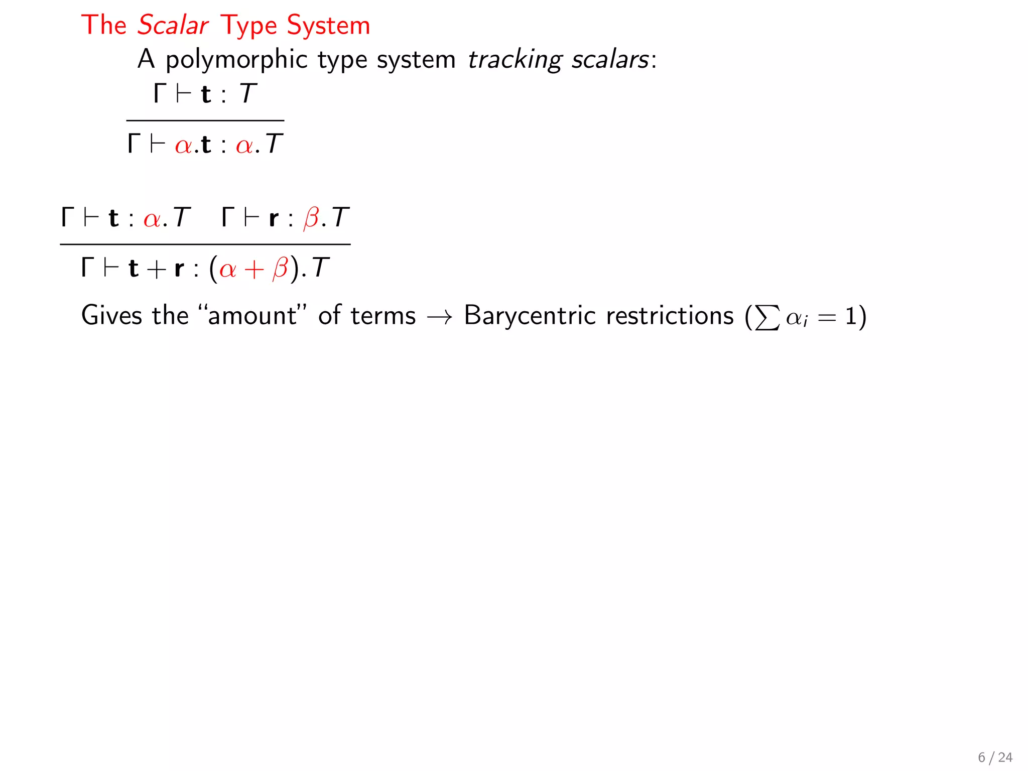
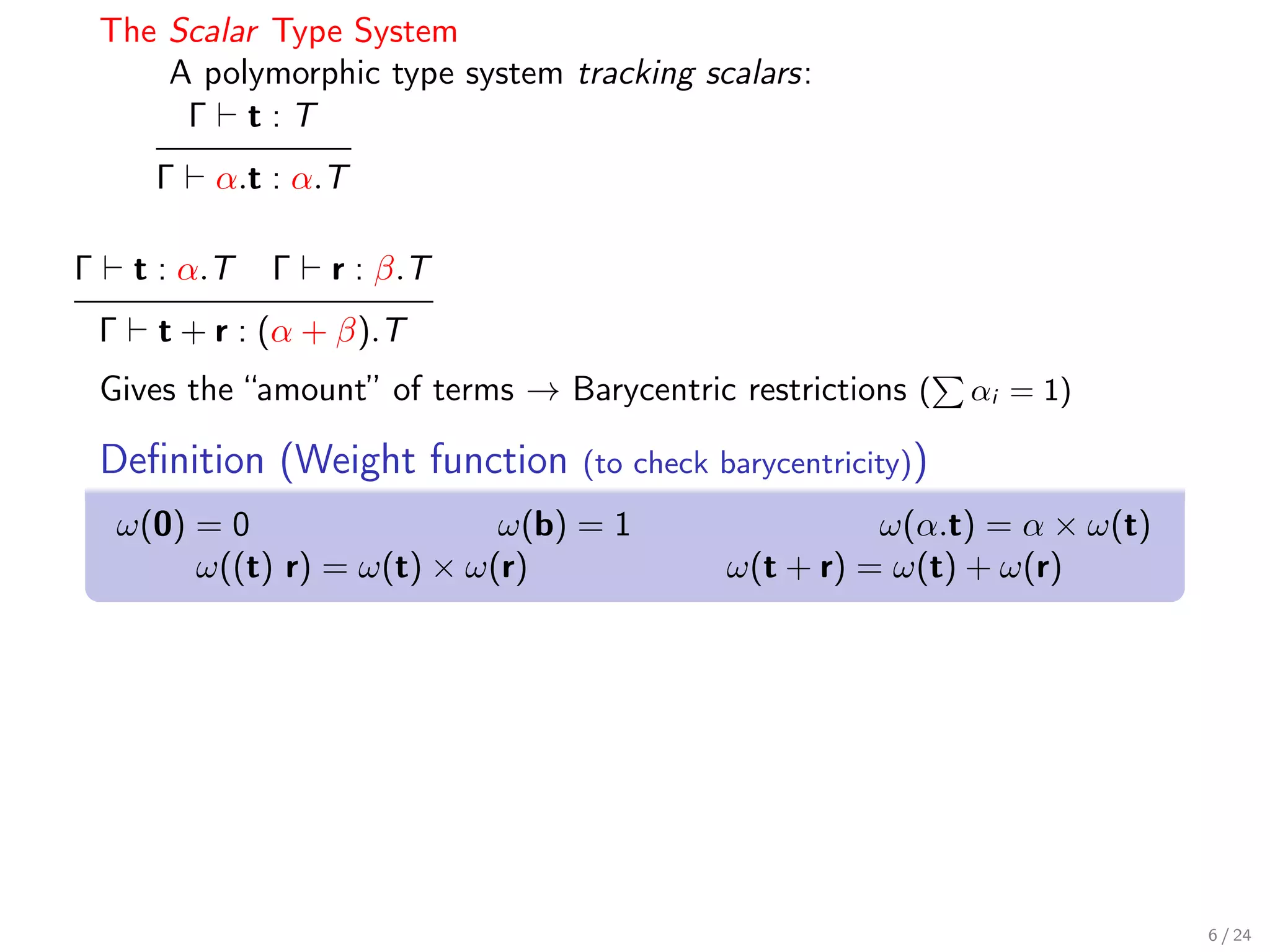
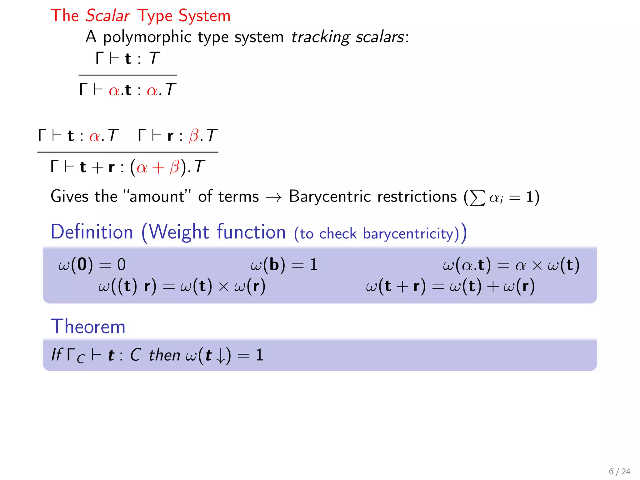
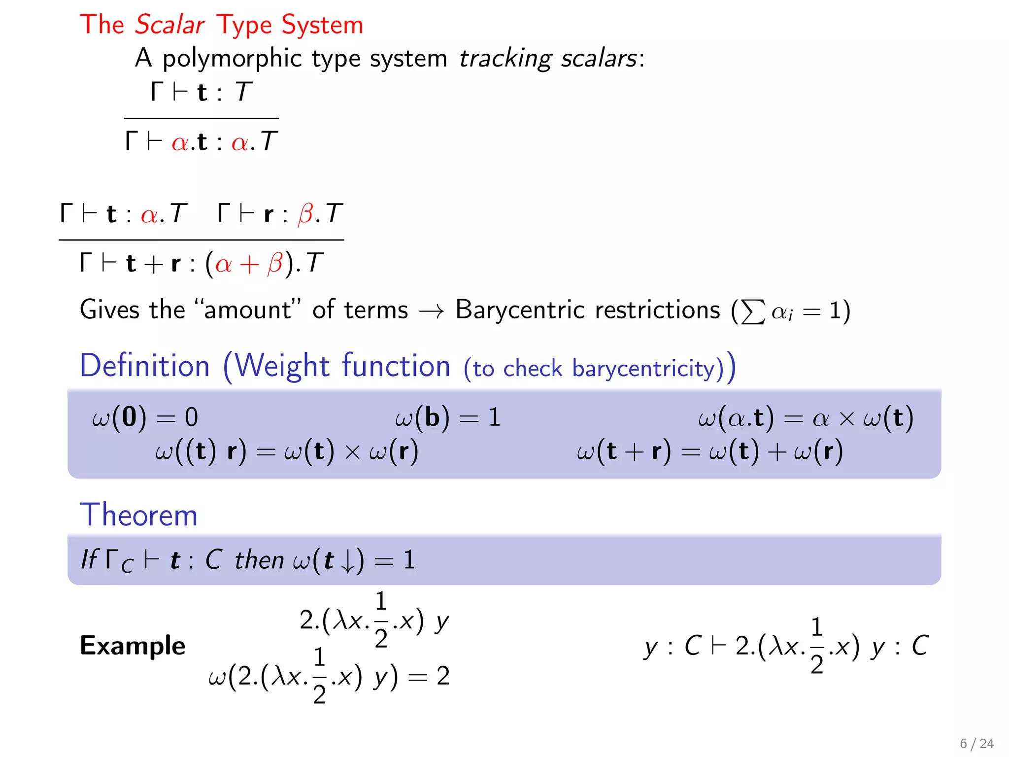
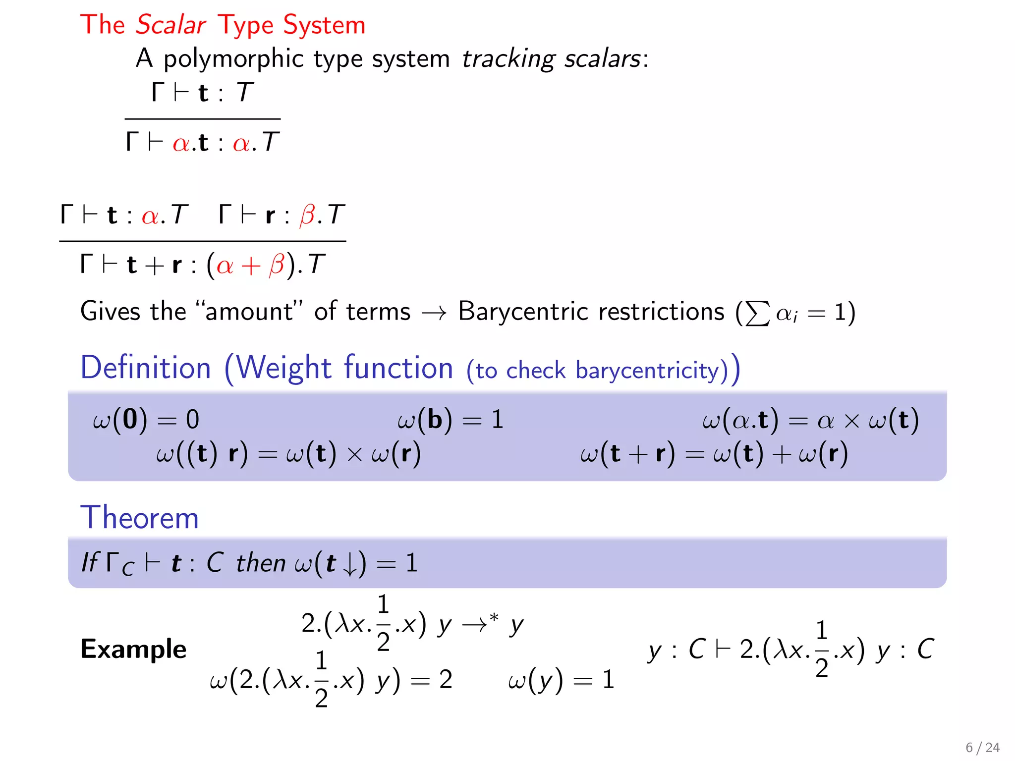
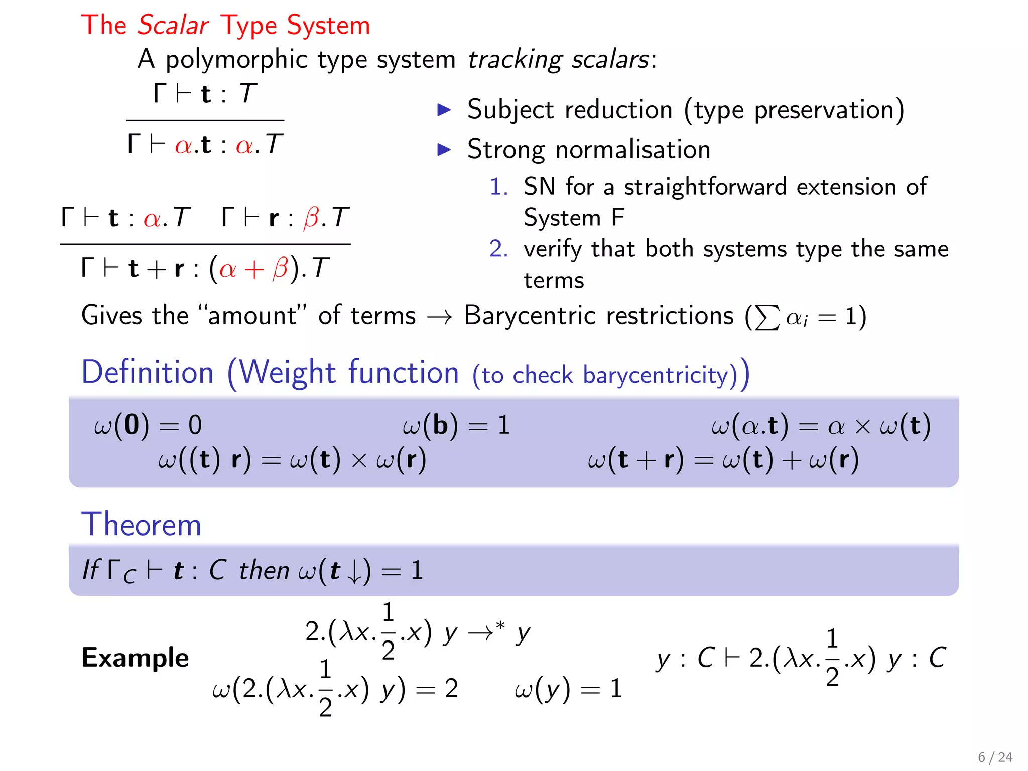
![The Scalar Type System
A polymorphic type system tracking scalars:
Γ t:T
Subject reduction (type preservation)
Γ α.t : α.T Strong normalisation
1. SN for a straightforward extension of
Γ t : α.T Γ r : β.T System F
2. verify that both systems type the same
Γ t + r : (α + β).T terms
Gives the “amount” of terms → Barycentric restrictions ( αi = 1)
Definition (Weight function (to check barycentricity))
ω(0) = 0 ω(b) = 1 ω(α.t) = α × ω(t)
ω((t) r) = ω(t) × ω(r) ω(t + r) = ω(t) + ω(r)
Theorem
If ΓC t : C then ω(t ↓) = 1
1
2.(λx. .x) y →∗ y 1
Example 2 y :C 2.(λx. .x) y : C
1 2
ω(2.(λx. .x) y ) = 2 ω(y ) = 1
2
Contribution: [Arrighi,Díaz-Caro’09]
6 / 24](https://image.slidesharecdn.com/du-typage-vectoriel-slides-120329081738-phpapp01/75/Slides-used-during-my-thesis-defense-Du-typage-vectoriel-24-2048.jpg)
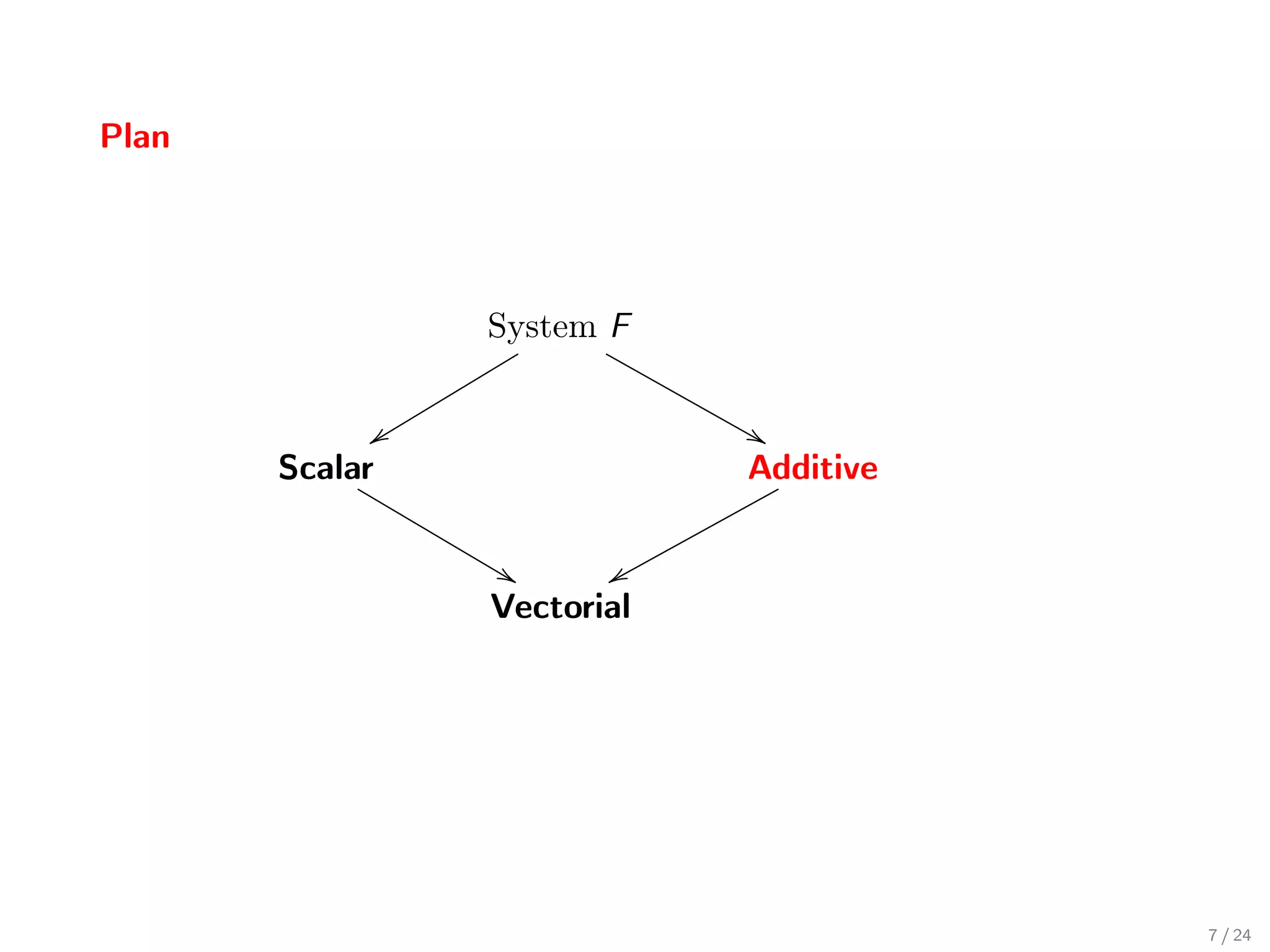
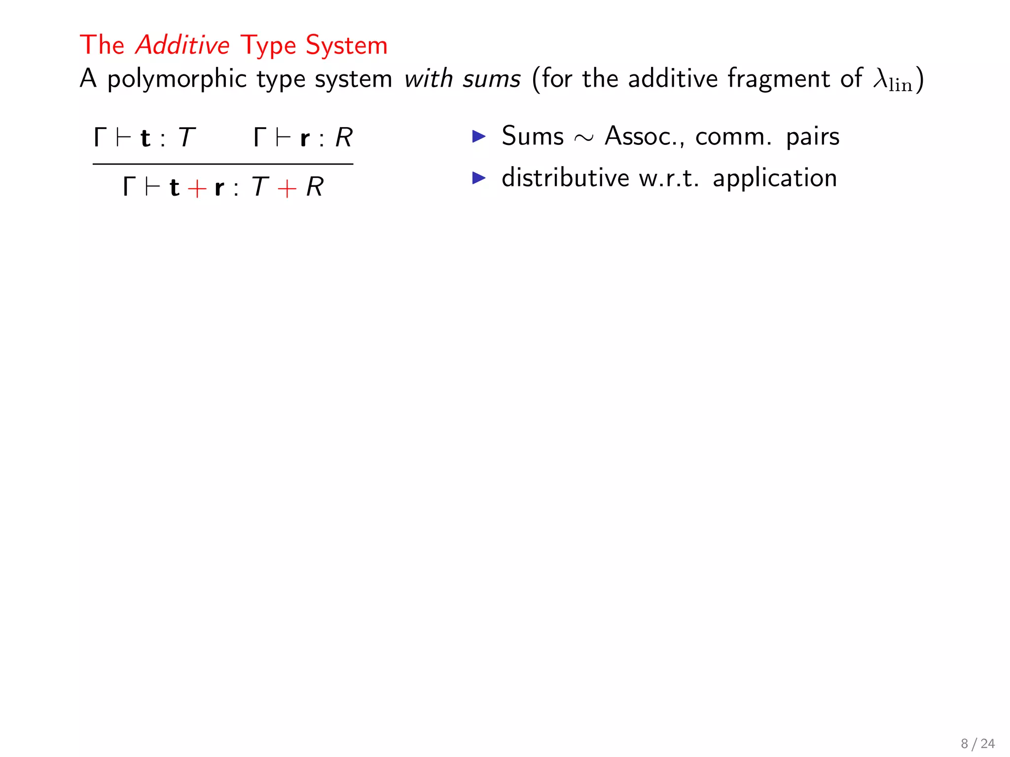
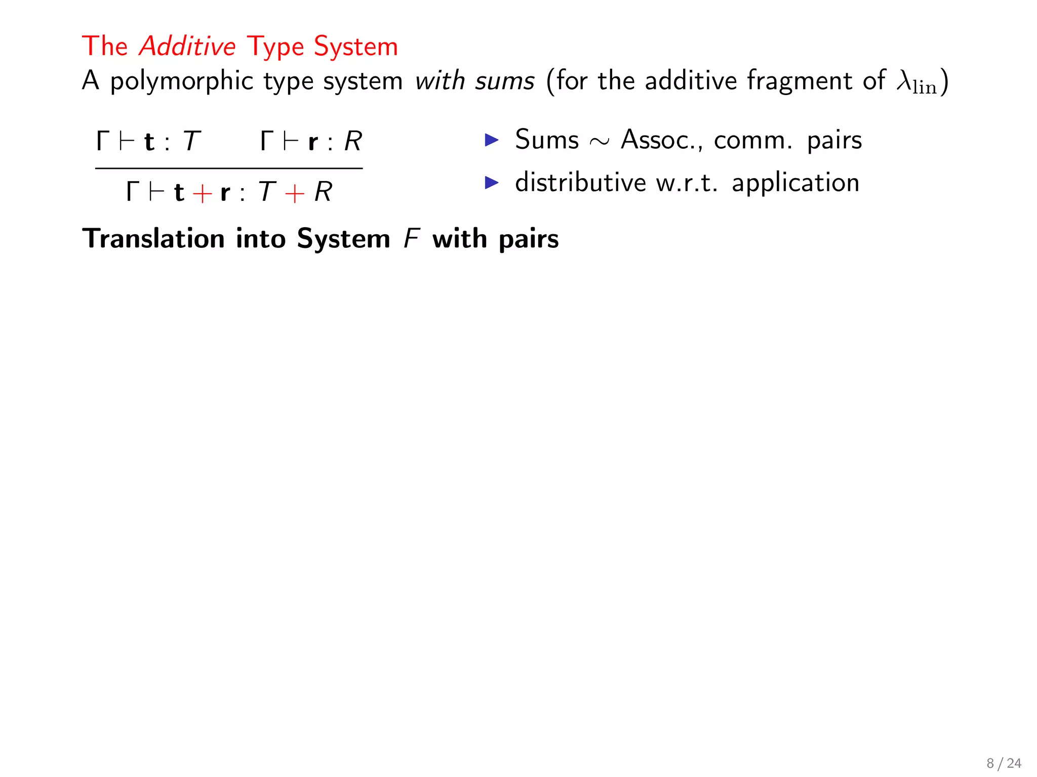
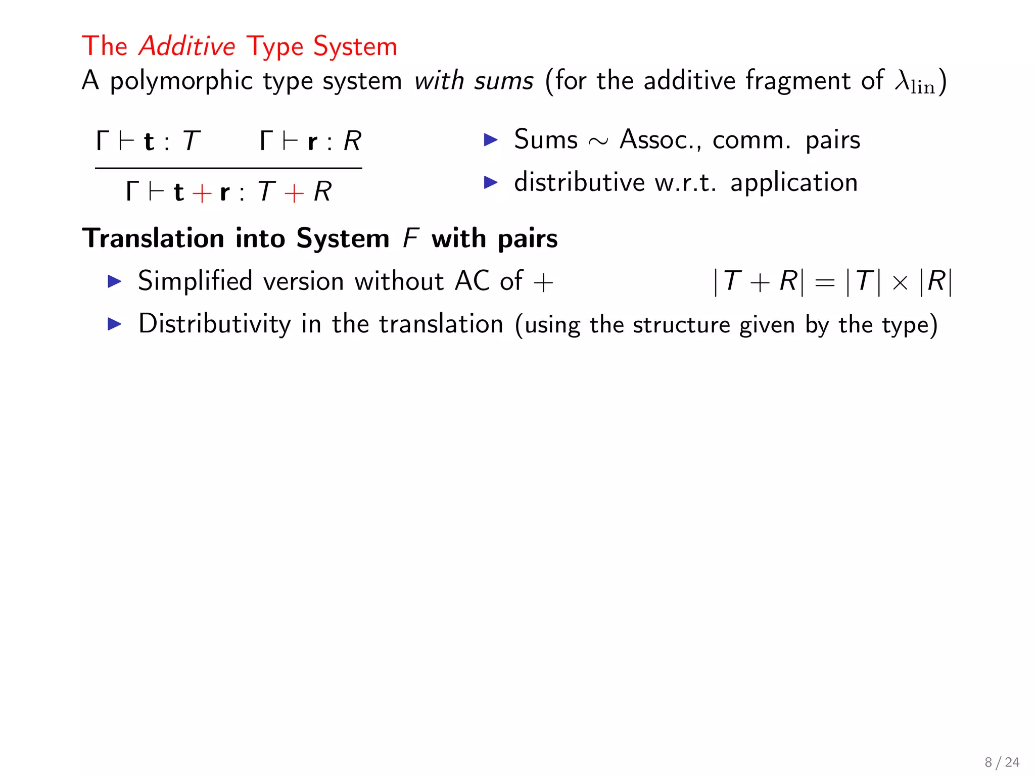
![The Additive Type System
A polymorphic type system with sums (for the additive fragment of λlin )
Γ t:T Γ r:R Sums ∼ Assoc., comm. pairs
Γ t+r:T +R distributive w.r.t. application
Translation into System F with pairs
Simplified version without AC of + |T + R| = |T | × |R|
Distributivity in the translation (using the structure given by the type)
Equivalences given explicitly: T ≡ R implies |T | ⇔ |R|
A×B ⇔B ×A (A × B) × C ⇔ A × (B × C )
Theorem
If Γ t : T and exists T ≡ T then |Γ| F [t]D : |T |
Also we set up an inverse translation showing that it is non-trivial
8 / 24](https://image.slidesharecdn.com/du-typage-vectoriel-slides-120329081738-phpapp01/75/Slides-used-during-my-thesis-defense-Du-typage-vectoriel-31-2048.jpg)
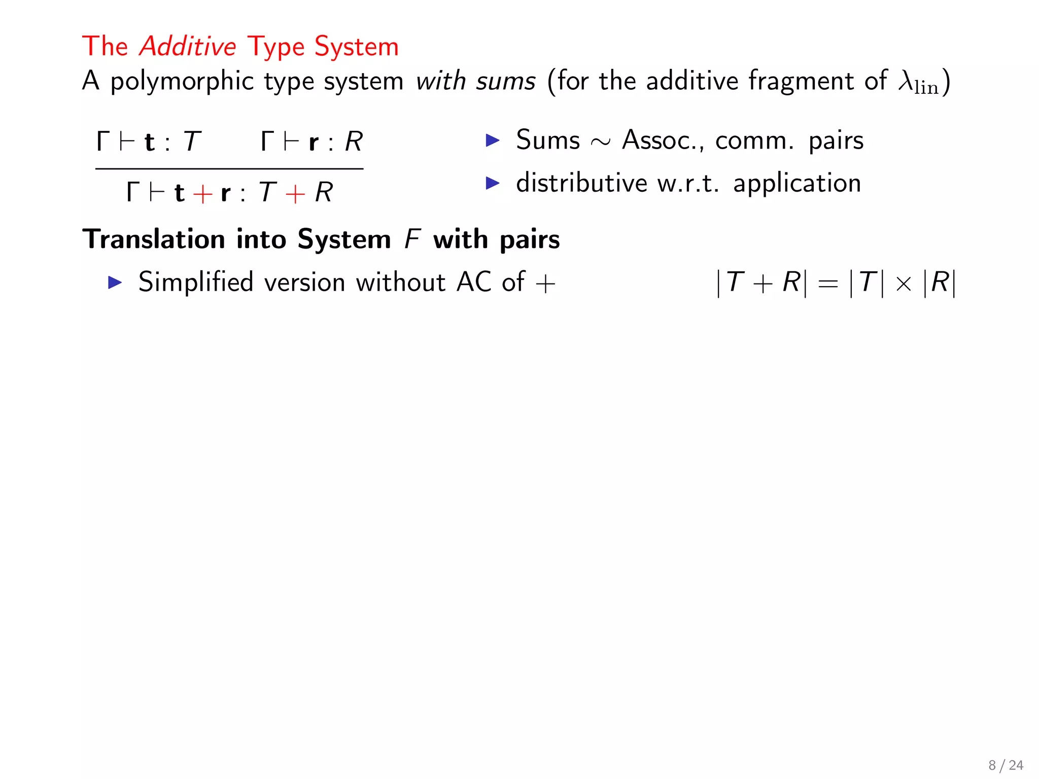
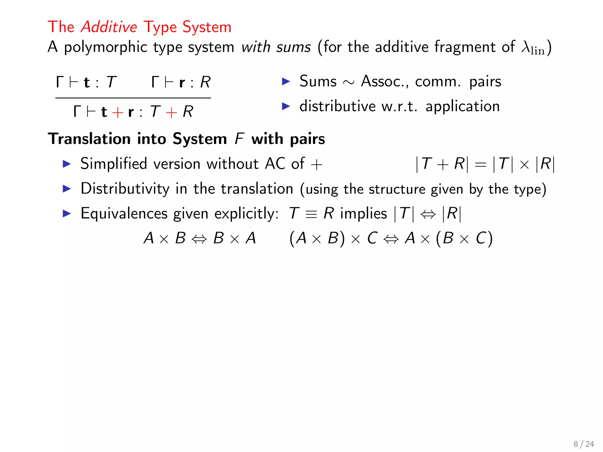
![The Additive Type System
A polymorphic type system with sums (for the additive fragment of λlin )
Γ t:T Γ r:R Sums ∼ Assoc., comm. pairs
Γ t+r:T +R distributive w.r.t. application
Translation into System F with pairs
Simplified version without AC of + |T + R| = |T | × |R|
Distributivity in the translation (using the structure given by the type)
Equivalences given explicitly: T ≡ R implies |T | ⇔ |R|
A×B ⇔B ×A (A × B) × C ⇔ A × (B × C )
Theorem
If Γ t : T and exists T ≡ T then |Γ| F [t]D : |T |
Also we set up an inverse translation showing that it is non-trivial
Subject reduction
Strong normalisation (using the one from System Fp )
Contribution: [Díaz-Caro,Petit’10]
8 / 24](https://image.slidesharecdn.com/du-typage-vectoriel-slides-120329081738-phpapp01/75/Slides-used-during-my-thesis-defense-Du-typage-vectoriel-32-2048.jpg)
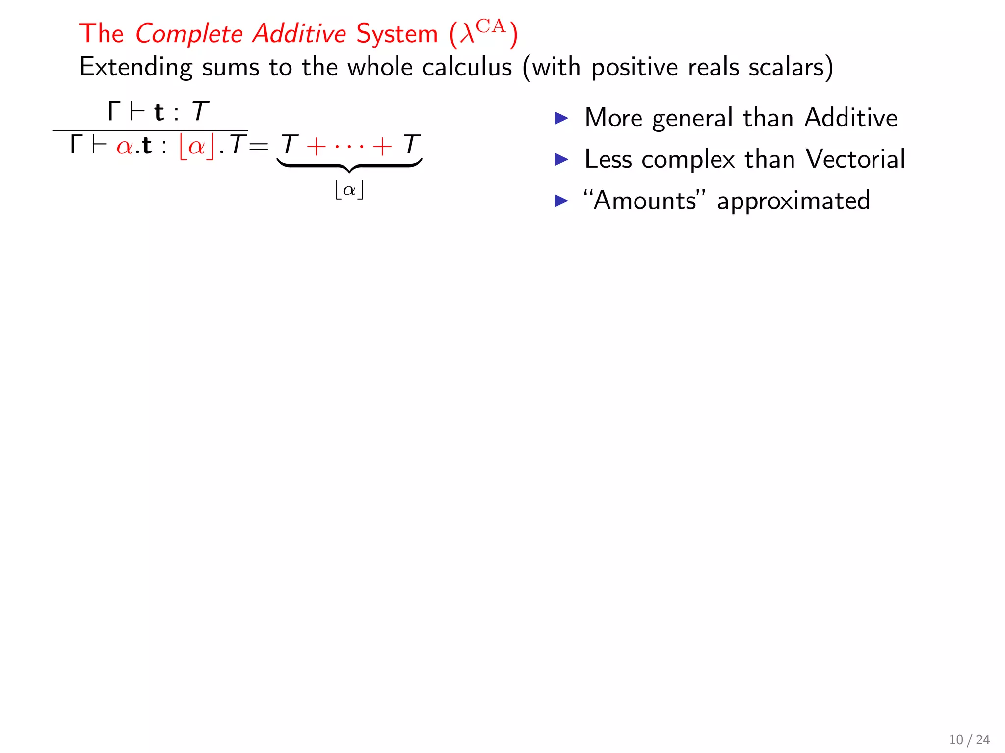
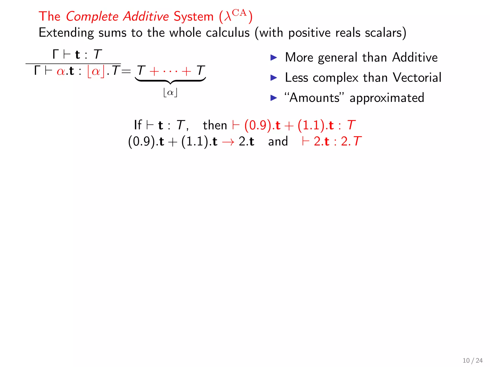
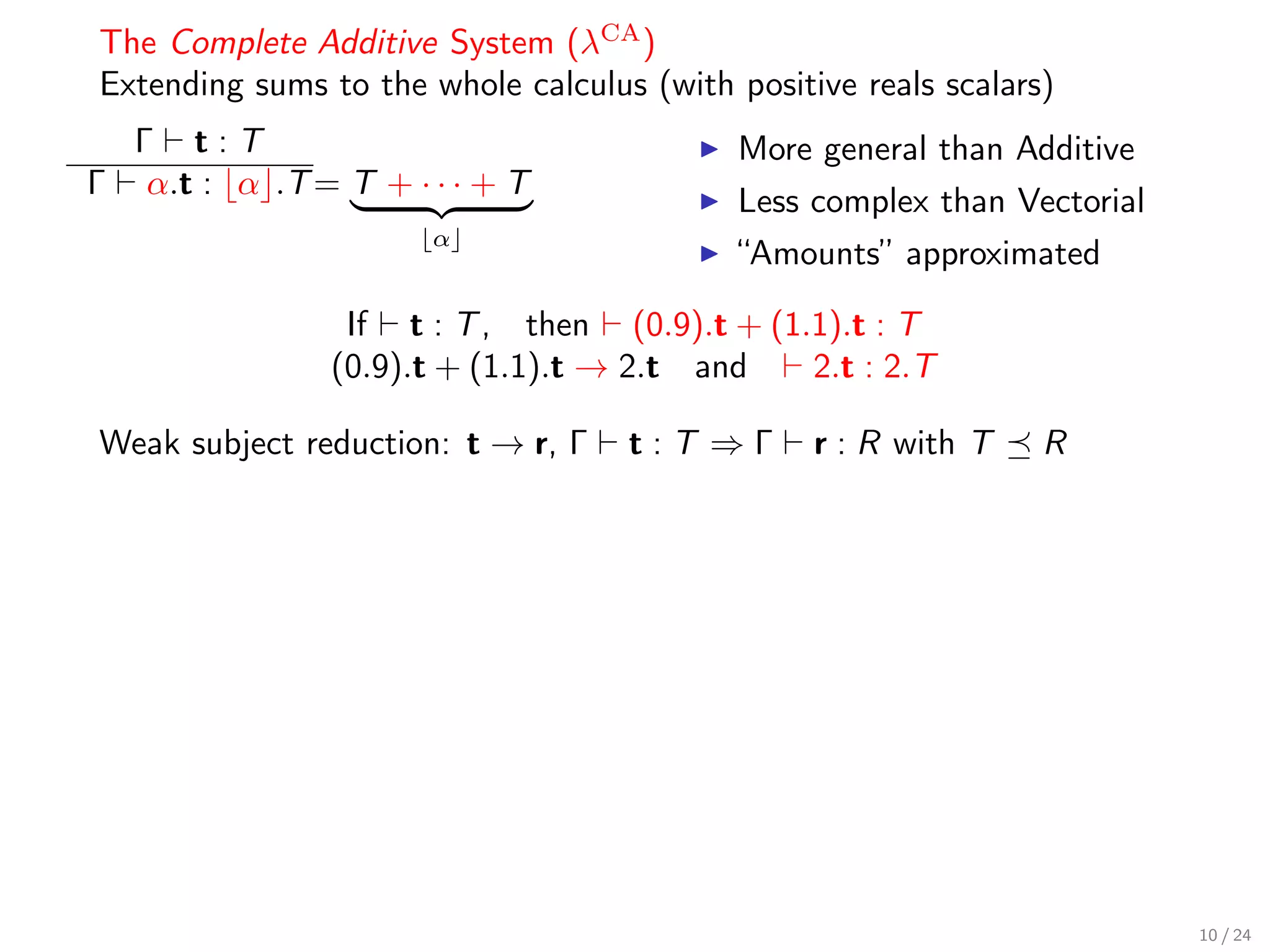
![The Complete Additive System (λCA )
Extending sums to the whole calculus (with positive reals scalars)
Γ t:T More general than Additive
Γ α.t : α .T = T + · · · + T
Less complex than Vectorial
α
“Amounts” approximated
If t : T , then (0.9).t + (1.1).t : T
(0.9).t + (1.1).t → 2.t and 2.t : 2.T
Weak subject reduction: t → r, Γ t : T ⇒ Γ r : R with T R
Abstract interpretation (theorem)
[·]
λCA
τ / λadd / Fp
↓ ↓a ↓F
( ) ( )
λCA / λadd / Fp
τ [·]
10 / 24](https://image.slidesharecdn.com/du-typage-vectoriel-slides-120329081738-phpapp01/75/Slides-used-during-my-thesis-defense-Du-typage-vectoriel-38-2048.jpg)
![The Complete Additive System (λCA )
Extending sums to the whole calculus (with positive reals scalars)
Γ t:T More general than Additive
Γ α.t : α .T = T + · · · + T
Less complex than Vectorial
α
“Amounts” approximated
If t : T , then (0.9).t + (1.1).t : T
(0.9).t + (1.1).t → 2.t and 2.t : 2.T
Weak subject reduction: t → r, Γ t : T ⇒ Γ r : R with T R
Abstract interpretation (theorem)
[·]
λCA
τ / λadd / Fp
↓ ↓a ↓F
( ) ( )
λCA / λadd / Fp
τ [·]
Strong normalisation (using Additive)
Contribution: [Buiras,Díaz-Caro,Jaskelioff’11]
10 / 24](https://image.slidesharecdn.com/du-typage-vectoriel-slides-120329081738-phpapp01/75/Slides-used-during-my-thesis-defense-Du-typage-vectoriel-39-2048.jpg)
![Typing rules
Γ t:T Γ t:T
ax 0I sI
Γ, x : U x :U Γ 0 : 0.T Γ α.t : α.T
n m
∀Vj , ∃Wj /
Γ t: αi .∀X .(U → Ti ) Γ r: βj .Vj U[Wj /X ] = Vj
i=1 j=1
→E
n m
Γ (t) r : αi × βj .Ti [Wj /X ]
i=1 j=1
Γ, x : U t:T Γ t:T Γ r:R
→I +I
Γ λx.t : U → T Γ t+r:T +R
n n
Γ t: αi .Ui X ∈ FV (Γ)
/ Γ t: αi .∀X .Ui
i=1 i=1
∀I ∀E
n n
Γ t: αi .∀X .Ui Γ t: αi .Ui [V /X ]
i=1 i=1
13 / 24](https://image.slidesharecdn.com/du-typage-vectoriel-slides-120329081738-phpapp01/75/Slides-used-during-my-thesis-defense-Du-typage-vectoriel-42-2048.jpg)
![Typing rules
Γ t:T Γ t:T
ax 0I sI
Γ, x : U x :U Γ 0 : 0.T Γ α.t : α.T
n m
∀Vj , ∃Wj /
Γ t: αi .∀X .(U → Ti ) Γ r: βj .Vj U[Wj /X ] = Vj
i=1 j=1
→E
n m
Γ (t) r : αi × βj .Ti [Wj /X ]
i=1 j=1
Γ, x : U t:T Γ t:T Γ r:R
→I +I
Γ λx.t : U → T Γ t+r:T +R
n n
Γ t: αi .Ui X ∈ FV (Γ)
/ Γ t: αi .∀X .Ui
i=1 i=1
∀I ∀E
n n
Γ t: αi .∀X .Ui Γ t: αi .Ui [V /X ]
i=1 i=1
Strong normalisation: Reducibility candidates
Main difficulty: show that {ti }i SN ⇒ i ti SN (algebraic measure)
13 / 24](https://image.slidesharecdn.com/du-typage-vectoriel-slides-120329081738-phpapp01/75/Slides-used-during-my-thesis-defense-Du-typage-vectoriel-43-2048.jpg)
![Typing rules
Γ t:T Γ t:T
ax 0I sI
Γ, x : U x :U Γ 0 : 0.T Γ α.t : α.T
n m
∀Vj , ∃Wj /
Γ t: αi .∀X .(U → Ti ) Γ r: βj .Vj U[Wj /X ] = Vj
i=1 j=1
→E
n m
Γ (t) r : αi × βj .Ti [Wj /X ]
i=1 j=1
Γ, x : U t:T Γ t:T Γ r:R
→I +I
Γ λx.t : U → T Γ t+r:T +R
n n
Γ t: αi .Ui X ∈ FV (Γ)
/ Γ t: αi .∀X .Ui
i=1 i=1
∀I ∀E
n n
Γ t: αi .∀X .Ui Γ t: αi .Ui [V /X ]
i=1 i=1
Strong normalisation: Reducibility candidates
Main difficulty: show that {ti }i SN ⇒ i ti SN (algebraic measure)
Subject reduction a challenge
13 / 24](https://image.slidesharecdn.com/du-typage-vectoriel-slides-120329081738-phpapp01/75/Slides-used-during-my-thesis-defense-Du-typage-vectoriel-44-2048.jpg)
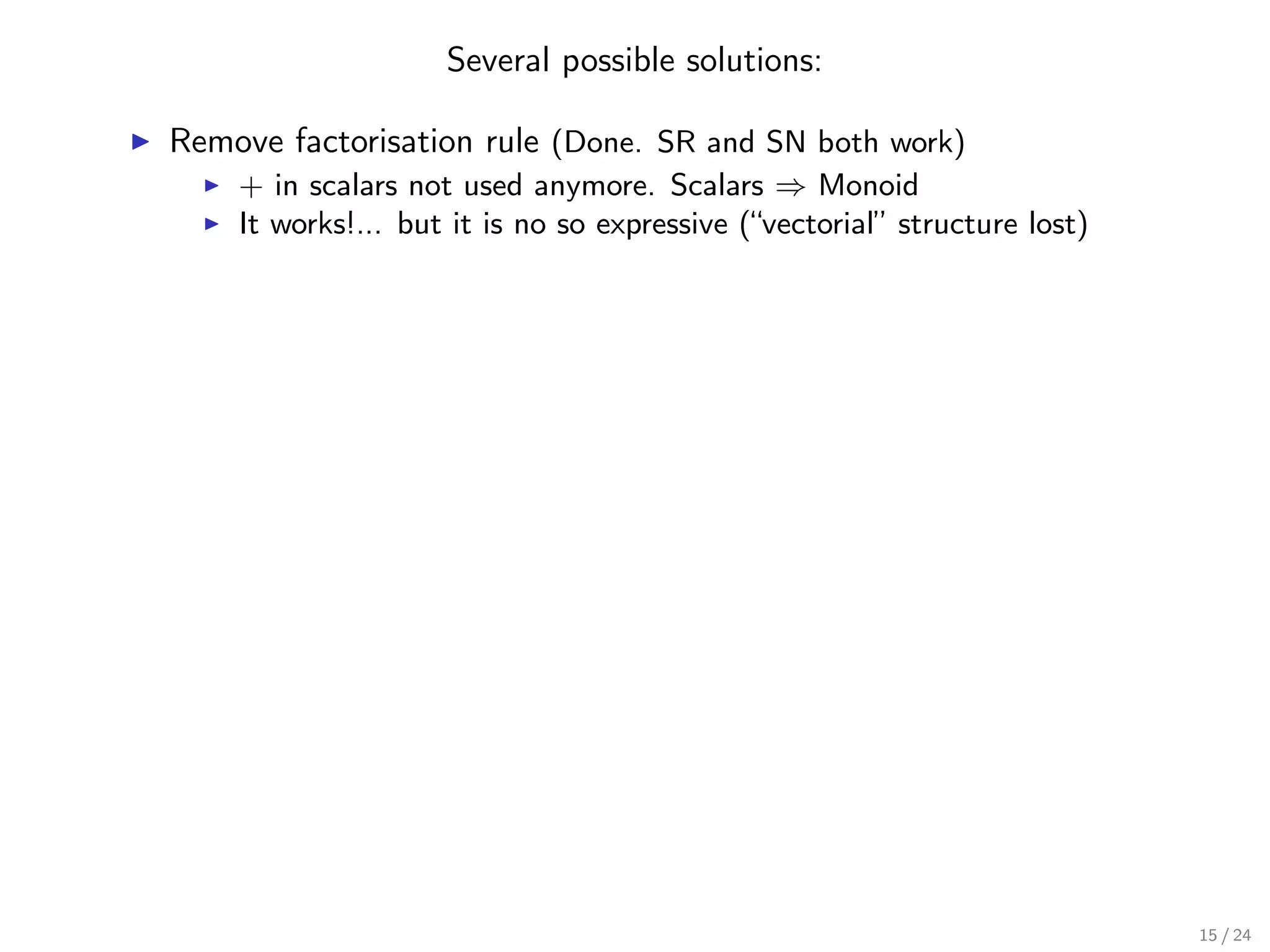
![Several possible solutions:
Remove factorisation rule (Done. SR and SN both work)
+ in scalars not used anymore. Scalars ⇒ Monoid
It works!... but it is no so expressive (“vectorial” structure lost)
Γ t:T Γ t:T
Add the typing rule
Γ (α + β).t : α.T + β.T
As soon as we add this one, we have to add many others
Too complex and inelegant (subject reduction by axiom)
Weak subject reduction
If Γ t : T and t →R r, then
if R is not the factorisation rule: Γ r : T
if R is the factorisation rule: ∃S T /Γ r:S
where (α + β).T α.T + β.T if ∃t / Γ t : T and Γ t:T
Contribution: [Arrighi,Díaz-Caro,Valiron’11]
15 / 24](https://image.slidesharecdn.com/du-typage-vectoriel-slides-120329081738-phpapp01/75/Slides-used-during-my-thesis-defense-Du-typage-vectoriel-48-2048.jpg)
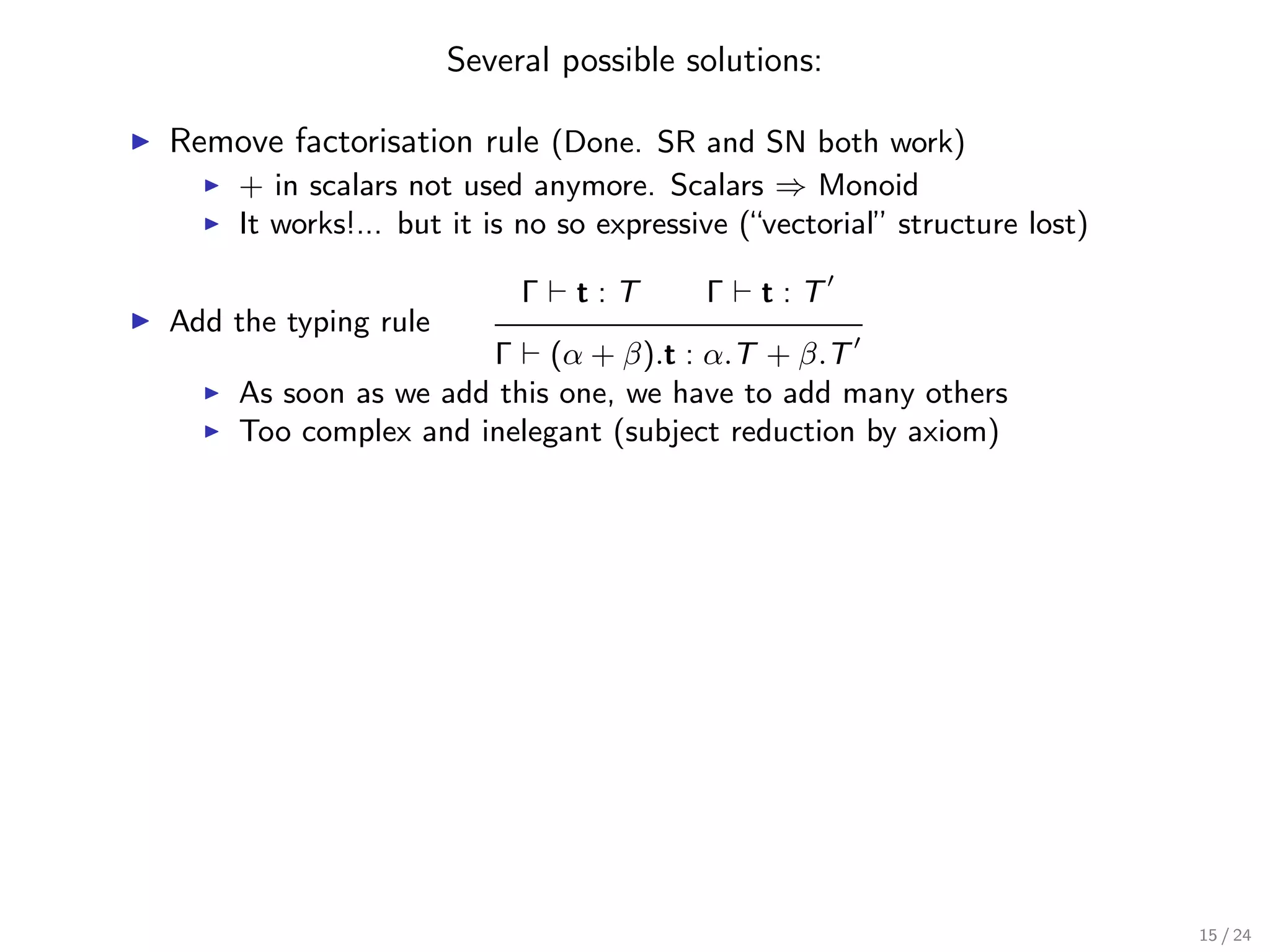
![Several possible solutions:
Remove factorisation rule (Done. SR and SN both work)
+ in scalars not used anymore. Scalars ⇒ Monoid
It works!... but it is no so expressive (“vectorial” structure lost)
Γ t:T Γ t:T
Add the typing rule
Γ (α + β).t : α.T + β.T
As soon as we add this one, we have to add many others
Too complex and inelegant (subject reduction by axiom)
Weak subject reduction
If Γ t : T and t →R r, then
if R is not the factorisation rule: Γ r : T
if R is the factorisation rule: ∃S T /Γ r:S
where (α + β).T α.T + β.T if ∃t / Γ t : T and Γ t:T
Contribution: [Arrighi,Díaz-Caro,Valiron’11]
Church style
Seems to be the natural solution: the type is part of the term, if the
types are different, the terms are different (no factorisation rule)
15 / 24](https://image.slidesharecdn.com/du-typage-vectoriel-slides-120329081738-phpapp01/75/Slides-used-during-my-thesis-defense-Du-typage-vectoriel-49-2048.jpg)
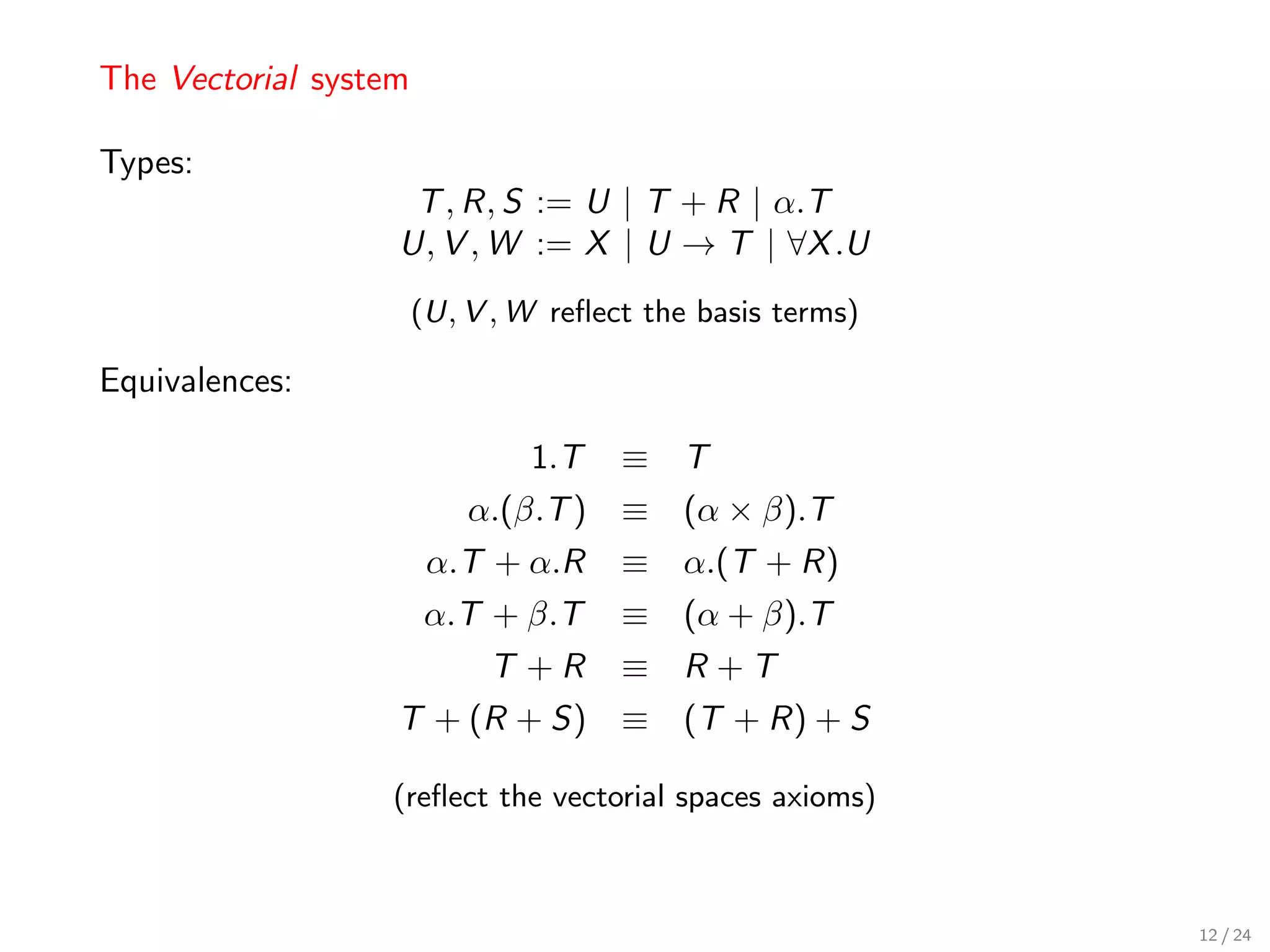
![The system Lineal
Types:
T , R, S := U | T + R | α.T
U, V , W := X | U → T | ∀X .U | U@( i Vi )
(U, V , W reflect the basis terms)
Equivalences:
1.T ≡ T
α.(β.T ) ≡ (α × β).T
α.T + α.R ≡ α.(T + R)
α.T + β.T ≡ (α + β).T
T +R ≡ R +T
T + (R + S) ≡ (T + R) + S
(∀X .U)@V ≡ U[V /X ]
(reflect the vectorial spaces axioms)
17 / 24](https://image.slidesharecdn.com/du-typage-vectoriel-slides-120329081738-phpapp01/75/Slides-used-during-my-thesis-defense-Du-typage-vectoriel-51-2048.jpg)
![Typing rules
Γ t:T Γ t:T
ax 0I sI
Γ, x : U x :U Γ 0 : 0.T Γ α.t : α.T
n m+δ m
∀Vj , ∃j1 , . . . , jk /
Γ t: αi .( ∀X k .(U → Ti ))@ Wj k Γ r: βj .Vj U [Wj /X ] = Vj
k
i=1 j=1 j=1
→E
n m
Γ (t) r : αi × βj .Ti [Wj /X ] k
i=1 j=1
Γ, x : U t:T Γ t:T Γ r:R
→I +I
Γ λx : U.t : U → T Γ t+r:T +R
n n
Γ t: αi .Ui X ∈ FV (Γ)
/ Γ t: αi .∀X .Ui
i=1 i=1
∀I @I
n m n m
Γ ΛX .t : αi .∀X .Ui Γ t@( Vj ) : αi .(∀X .Ui )@( Vj )
i=1 j=1 i=1 j=1
Subject reduction
Strong normalisation (using Vectorial)
18 / 24](https://image.slidesharecdn.com/du-typage-vectoriel-slides-120329081738-phpapp01/75/Slides-used-during-my-thesis-defense-Du-typage-vectoriel-52-2048.jpg)
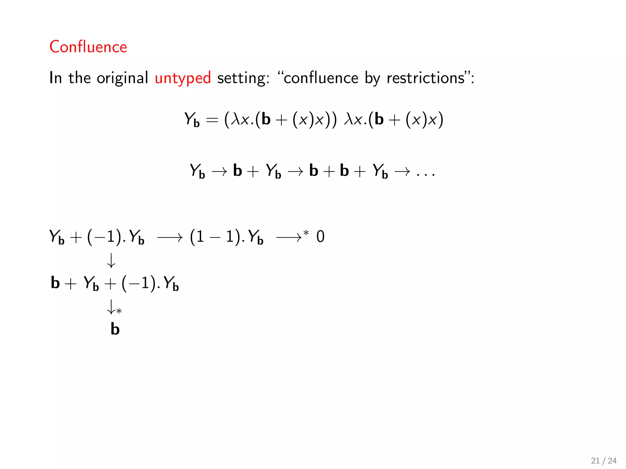
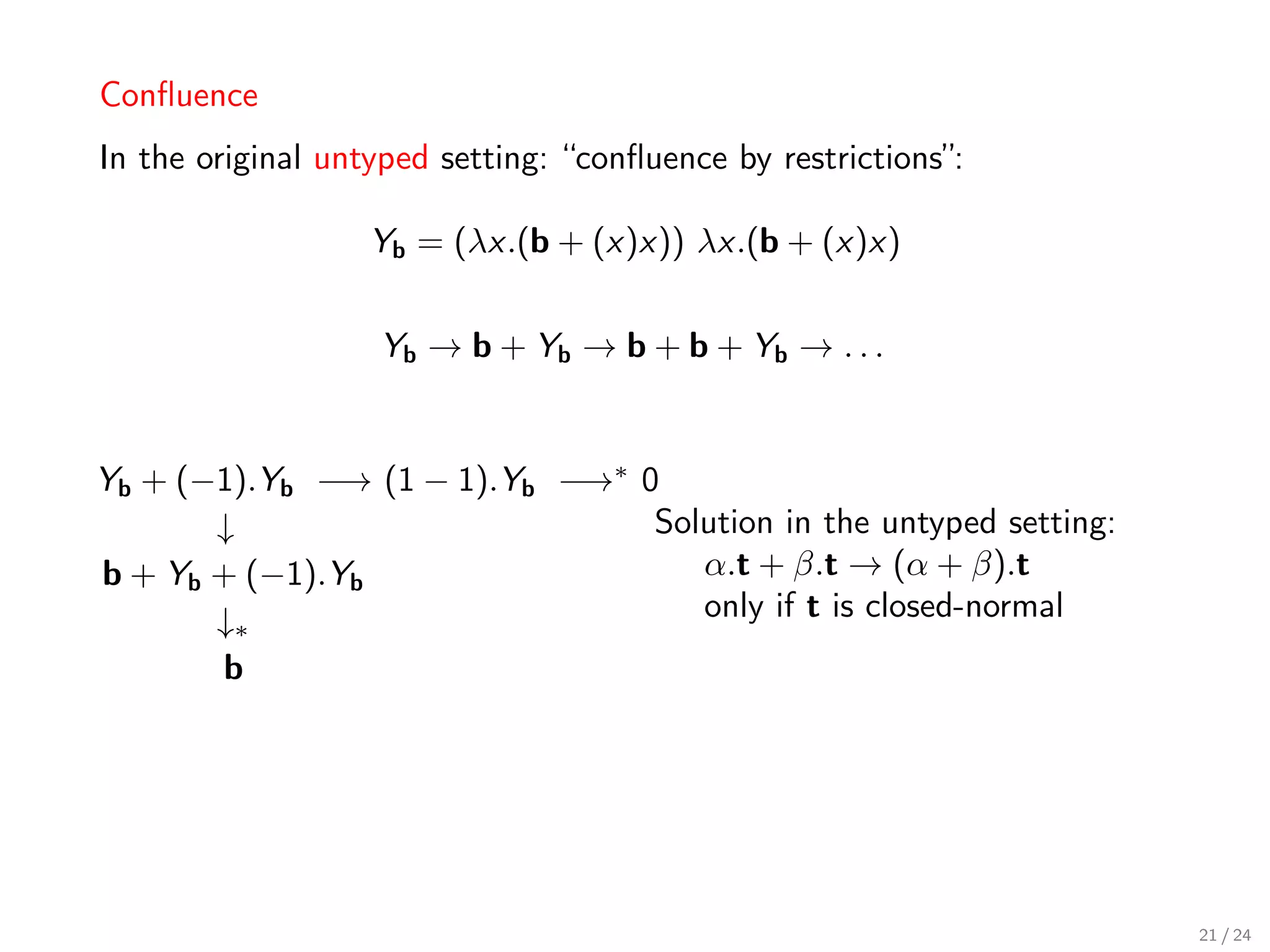
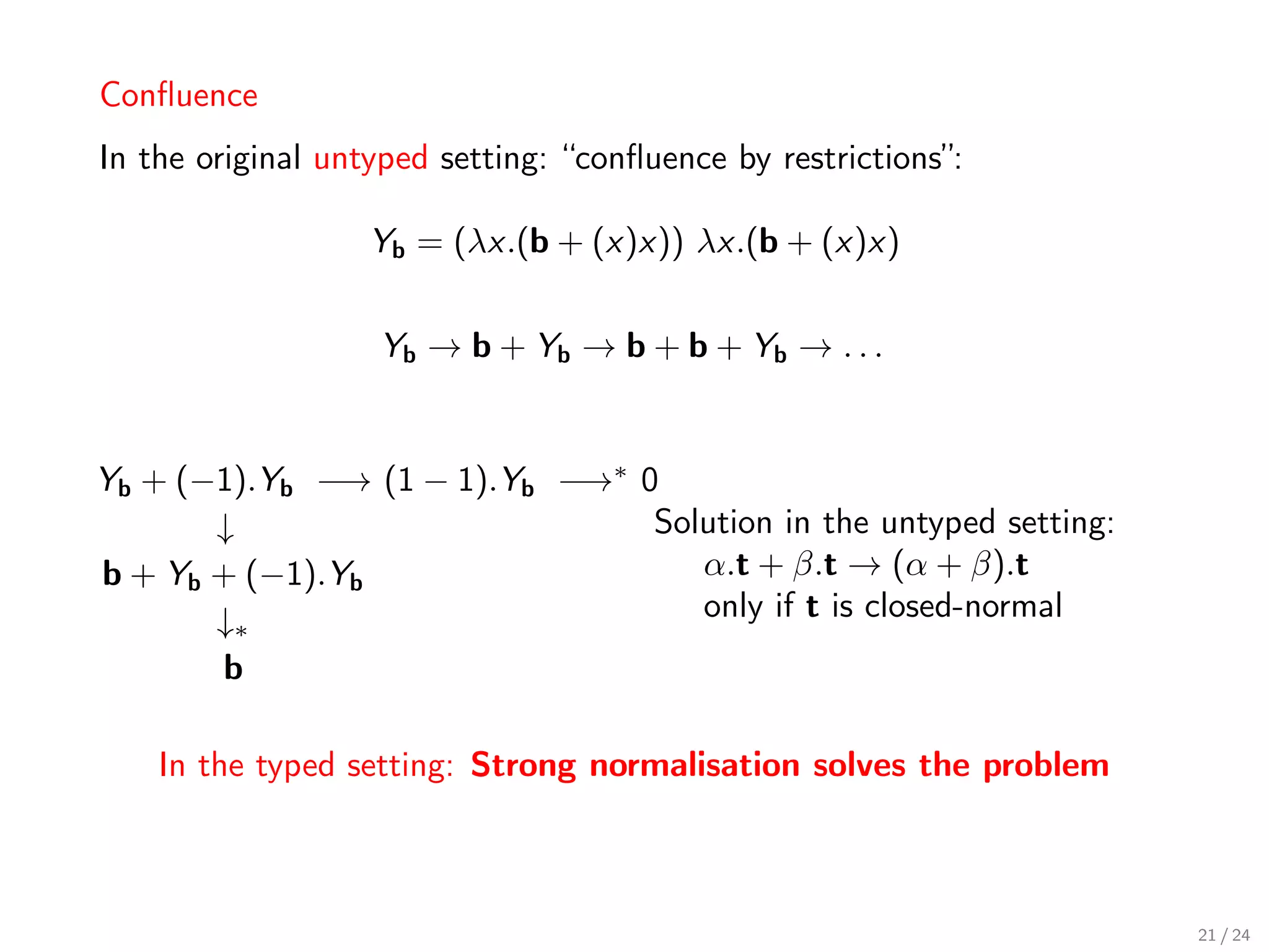
![Theorem (Confluence)
∀t / Γ t:T ∗
t ∗
r1 r2
∗ ~ ∗
s
Proof.
1) local confluence: t
r1 r2
∗ ~ ∗
s
Algebraic fragment: Coq proof [Valiron’10]
Beta-reduction: Straightforward extension
Commutation: Induction
2) Local confluence + Strong normalisation ⇒ Confluence
22 / 24](https://image.slidesharecdn.com/du-typage-vectoriel-slides-120329081738-phpapp01/75/Slides-used-during-my-thesis-defense-Du-typage-vectoriel-59-2048.jpg)
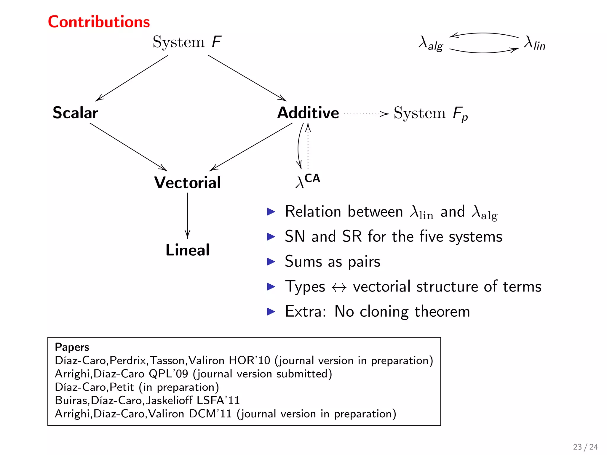
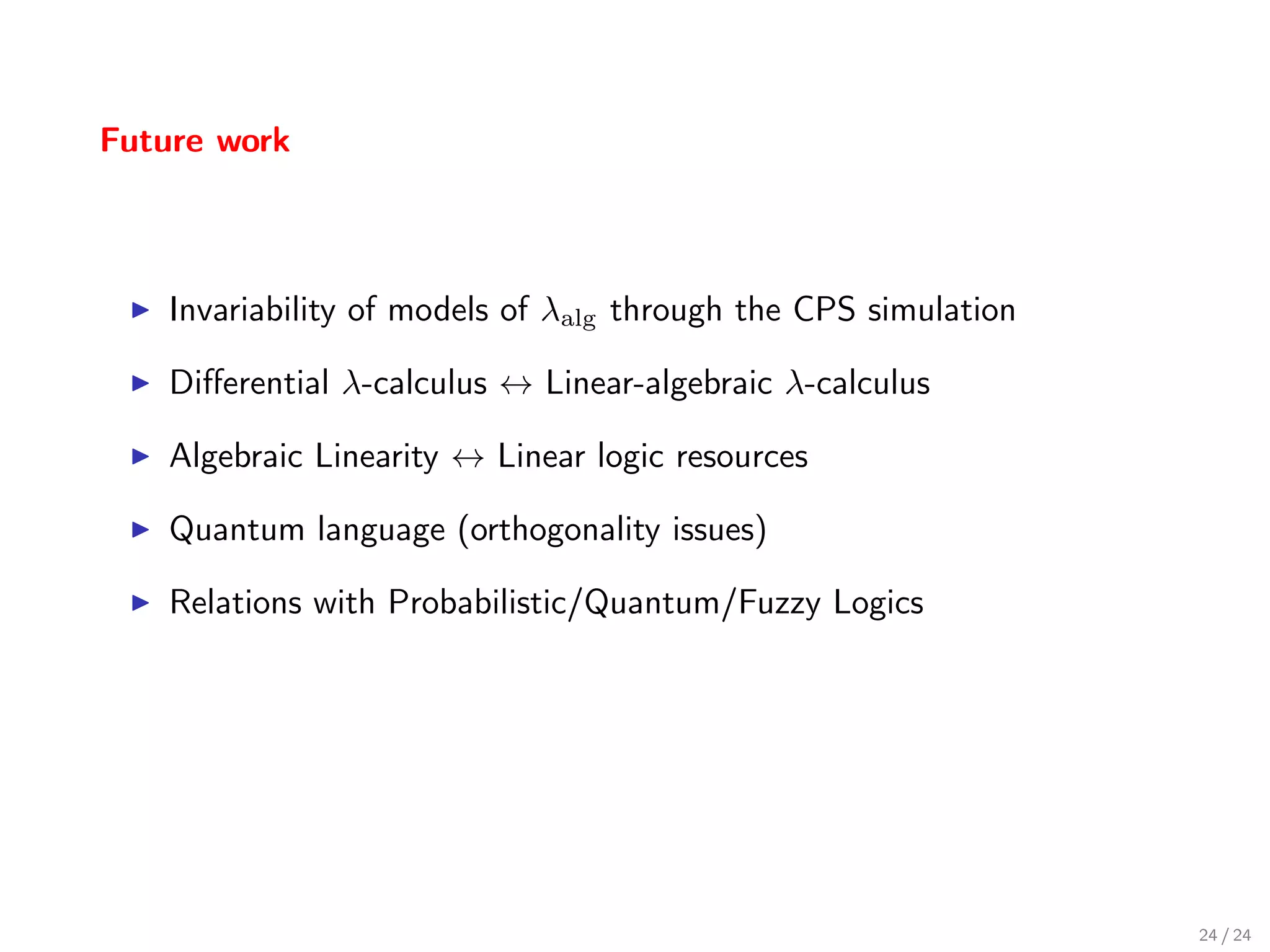

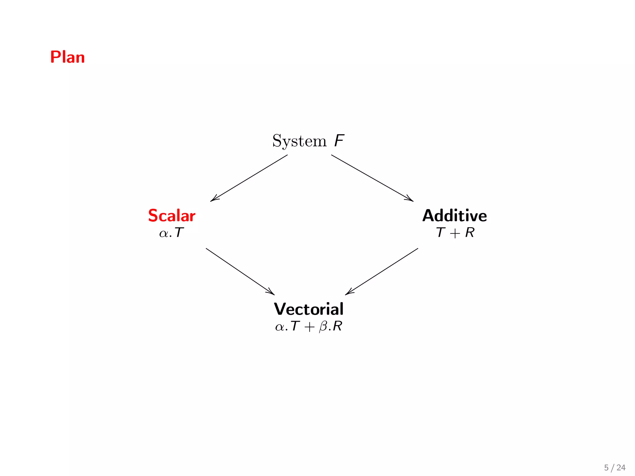
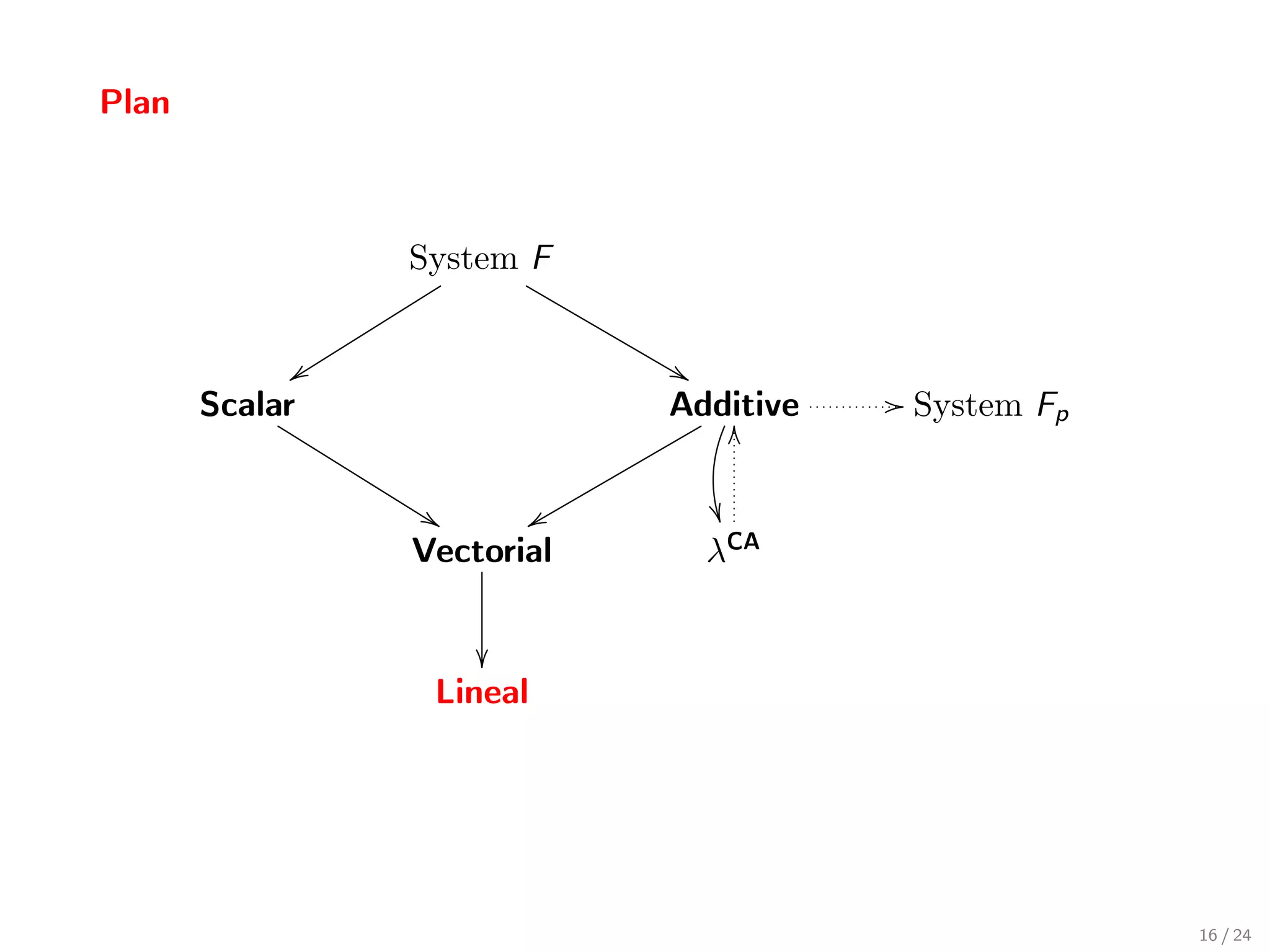
The document outlines the thesis defense by Alejandro Díaz-Caro, focusing on vectorial typing in lambda calculus and its applications in capturing probabilistic and quantum structures. It details various type systems, including System F and algebraic extensions, and discusses the relationships between type systems and logical frameworks, particularly the Curry-Howard correspondence. Additionally, it presents a polymorphic type system for tracking scalars and an additive type system, showcasing their capabilities in managing complex term structures.


![[FLOLAC'14][scm] Functional Programming Using Haskell](https://cdn.slidesharecdn.com/ss_thumbnails/slides-140630030216-phpapp01-thumbnail.jpg?width=640&height=640&fit=bounds)


![Coded Agents – with UiPath SDK + LangGraph [Virtual Hands-on Workshop]](https://cdn.slidesharecdn.com/ss_thumbnails/codedagentsdeck-251215155422-5497c599-thumbnail.jpg?width=640&height=640&fit=bounds)


