Downloaded 61 times
![Equality Check
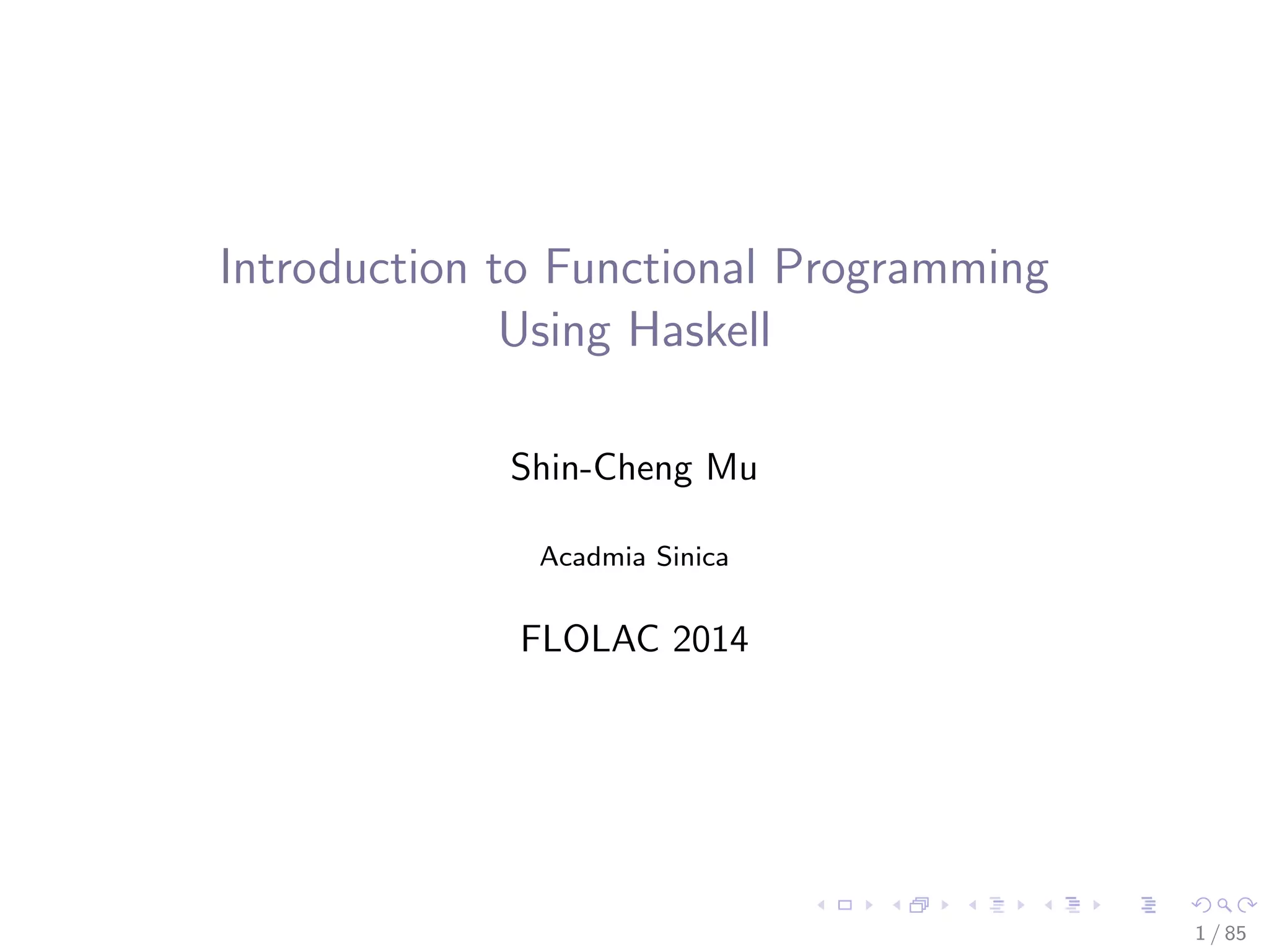
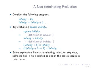
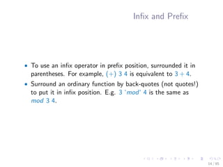
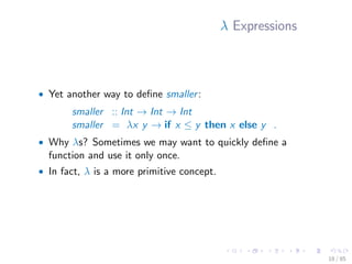
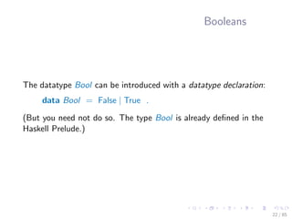
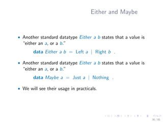
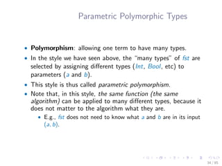
• You might have also noticed that we can check for equality of
a number of types:
• (==) :: Char → Char → Bool,
• (==) :: Int → Int → Bool,
• (==) :: (Int, Char) → (Int, Char) → Bool,
• (==) :: [Int] → [Int] → Bool . . .
• It differs from the situation of fst: the algorithm for checking
equality for each type is different. We just use the same name
to refer to them, for convenience.
35 / 85](https://image.slidesharecdn.com/slides-140630030216-phpapp01/85/FLOLAC-14-scm-Functional-Programming-Using-Haskell-42-320.jpg)
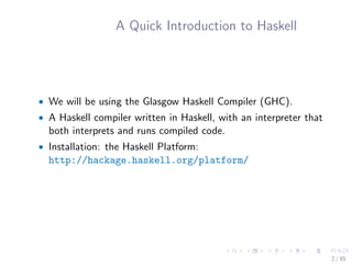
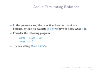
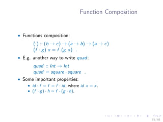
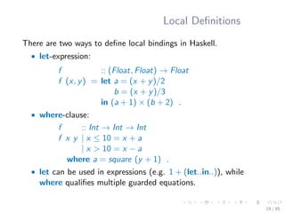
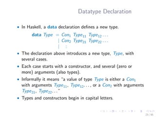
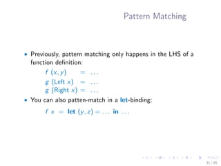
![Ad-Hoc Polymorphism
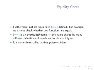
• Haskell deals with overloading by a general mechanism called
type classes. It is considered a major feature of Haskell.
• While the type class is an interesting topic, we might not
cover much of it since it is orthogonal to the central message
of this course.
• We only need to know that if a function uses (==), it is
noted in the type.
• E.g. The function pos x xs finds the position of the first
occurrence of x in xs. It needs to use equality check.
• It my have type pos :: Eq a ⇒ a → [a] → Int.
• Eq a says that “a cannot be any type. It should be a type for
which (==) is defined.”
37 / 85](https://image.slidesharecdn.com/slides-140630030216-phpapp01/85/FLOLAC-14-scm-Functional-Programming-Using-Haskell-44-320.jpg)
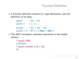
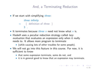
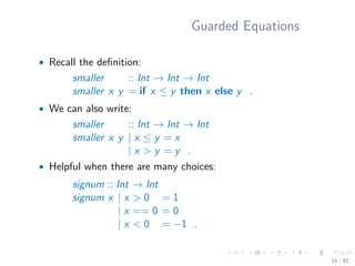
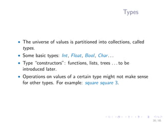
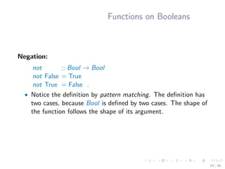
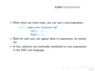
![Lists in Haskell
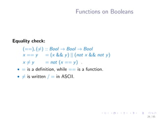
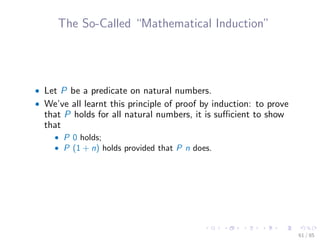
• Lists: conceptually, sequences of things.
• Traditionally an important datatype in functional languages.
• In Haskell, all elements in a list must be of the same type.
• [1, 2, 3, 4] :: [Int]
• [True, False, True] :: [Bool]
• [[1, 2], [ ], [6, 7]] :: [[Int]]
• [ ] :: [a], the empty list (whose element type is not determined).
38 / 85](https://image.slidesharecdn.com/slides-140630030216-phpapp01/85/FLOLAC-14-scm-Functional-Programming-Using-Haskell-45-320.jpg)
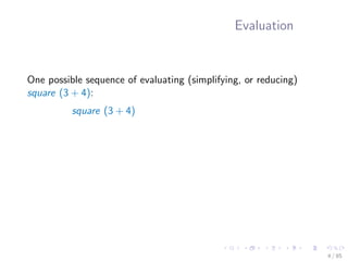
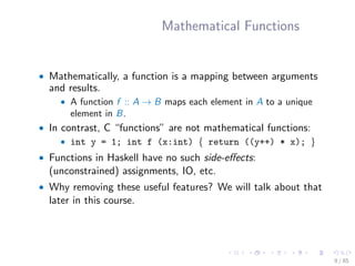
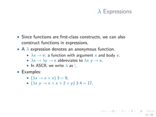
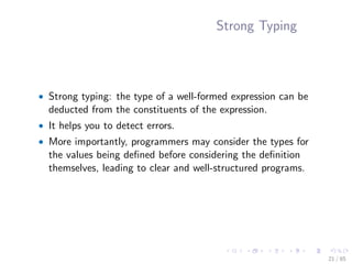
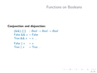
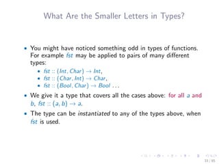
![List as a Datatype
• [ ] :: [a] is the empty list whose element type is not determined.
• If a list is non-empty, the leftmost element is called its head
and the rest its tail.
• The constructor (:) :: a → [a] → [a] builds a list. E.g. in
x : xs, x is the head and xs the tail of the new list.
• You can think of a list as being defined by
data [a] = [ ] | a : [a] .
• [1, 2, 3] is an abbreviation of 1 : (2 : (3 : [ ])).
39 / 85](https://image.slidesharecdn.com/slides-140630030216-phpapp01/85/FLOLAC-14-scm-Functional-Programming-Using-Haskell-46-320.jpg)
![Characters and Strings
• In Haskell, strings are treated as lists of characters.
• Thus when we write "abc", it is treated as an abbreviation of
['a', 'b', 'c'].
• It makes string processing convenient, while having some
efficiency issues.
• For efficiency, there are libraries providing “block”
representation of strings.
40 / 85](https://image.slidesharecdn.com/slides-140630030216-phpapp01/85/FLOLAC-14-scm-Functional-Programming-Using-Haskell-47-320.jpg)
![Head and Tail
• head :: [a] → a. e.g. head [1, 2, 3] = 1.
• tail :: [a] → [a]. e.g. tail [1, 2, 3] = [2, 3].
• init :: [a] → [a]. e.g. init [1, 2, 3] = [1, 2].
• last :: [a] → a. e.g. last [1, 2, 3] = 3.
• They are all partial functions on non-empty lists. e.g. head [ ]
crashes with an error message.
• null :: [a] → Bool checks whether a list is empty.
41 / 85](https://image.slidesharecdn.com/slides-140630030216-phpapp01/85/FLOLAC-14-scm-Functional-Programming-Using-Haskell-48-320.jpg)
![List Generation
• [0..25] generates the list [0, 1, 2..25].
• [0, 2..25] yields [0, 2, 4..24].
• [2..0] yields [].
• The same works for all ordered types. For example Char:
• ['a'..'z'] yields ['a', 'b', 'c'..'z'].
• [1..] yields the infinite list [1, 2, 3..].
42 / 85](https://image.slidesharecdn.com/slides-140630030216-phpapp01/85/FLOLAC-14-scm-Functional-Programming-Using-Haskell-49-320.jpg)
![List Comprehension
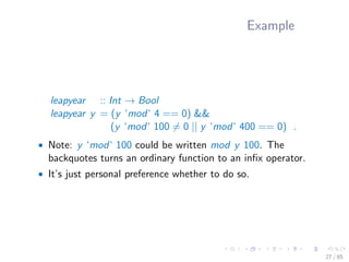
• Some functional languages provide a convenient notation for
list generation. It can be defined in terms of simpler functions.
• e.g. [x × x | x ← [1..5], odd x] = [1, 9, 25].
• Syntax: [e | Q1, Q2..]. Each Qi is either
• a generator x ← xs, where x is a (local) variable or pattern of
type a while xs is an expression yielding a list of type [a], or
• a guard, a boolean valued expression (e.g. odd x).
• e is an expression that can involve new local variables
introduced by the generators.
43 / 85](https://image.slidesharecdn.com/slides-140630030216-phpapp01/85/FLOLAC-14-scm-Functional-Programming-Using-Haskell-50-320.jpg)
![List Comprehension
Examples:
• [(a, b) | a ← [1..3], b ← [1..2]] =
[(1, 1), (1, 2), (2, 1), (2, 2), (3, 1), (3, 2)]
• [(a, b) | b ← [1..2], a ← [1..3]] =
[(1, 1), (2, 1), (3, 1), (1, 2), (2, 2), (3, 2)]
• [(i, j) | i ← [1..4], j ← [i + 1..4]] =
[(1, 2), (1, 3), (1, 4), (2, 3), (2, 4), (3, 4)]
• [(i, j) |← [1..4], even i, j ← [i + 1..4], odd j] = [(2, 3)]
44 / 85](https://image.slidesharecdn.com/slides-140630030216-phpapp01/85/FLOLAC-14-scm-Functional-Programming-Using-Haskell-51-320.jpg)
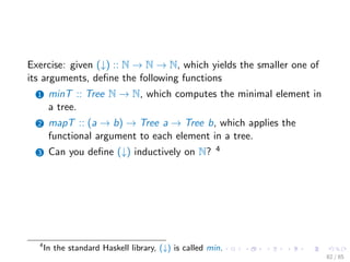
![Inductively Defined Lists
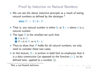
• Recall that a (finite) list can be seen as a datatype defined
by: 1
data [a] = [] | a : [a] .
• Every list is built from the base case [ ], with elements added
by (:) one by one: [1, 2, 3] = 1 : (2 : (3 : [ ])).
• The type [a] is the smallest set such that
1 [ ] is in [a];
2 if xs is in [a] and x is in a, x : xs is in [a] as well.
• In fact, Haskell allows you to build infinitely long lists (one
that never reaches [ ]). However. . .
• for now let’s consider finite lists only, as having infinite lists
make the semantics much more complicated. 2
1
Not a real Haskell definition.
2
What does that mean? We will talk about it later.
45 / 85](https://image.slidesharecdn.com/slides-140630030216-phpapp01/85/FLOLAC-14-scm-Functional-Programming-Using-Haskell-52-320.jpg)
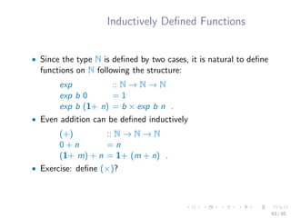
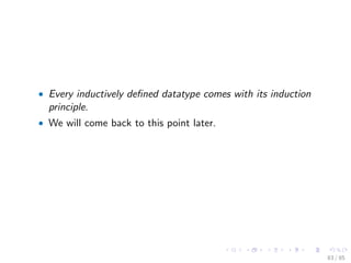
![Inductively Defined Functions on Lists
• Many functions on lists can be defined according to how a list
is defined:
sum :: [Int] → Int
sum [ ] = 0
sum (x : xs) = x + sum xs .
allEven :: Int → Bool
allEven [ ] = True
allEven f (x : xs) = even x && allEven xs .
46 / 85](https://image.slidesharecdn.com/slides-140630030216-phpapp01/85/FLOLAC-14-scm-Functional-Programming-Using-Haskell-53-320.jpg)
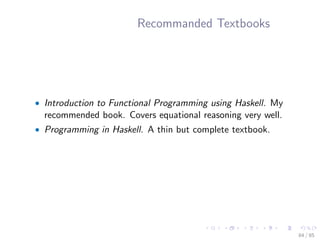
![Length
• The function length defined inductively:
length :: [a] → Int
length [ ] = 0
length (x : xs) = 1+ length xs .
47 / 85](https://image.slidesharecdn.com/slides-140630030216-phpapp01/85/FLOLAC-14-scm-Functional-Programming-Using-Haskell-54-320.jpg)
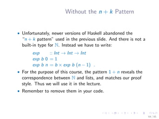
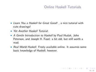
![List Append
• The function (++) appends two lists into one
(++) :: [a] → [a] → [a]
[ ] ++ ys = ys
(x : xs) ++ ys = x : (xs ++ ys) .
• Examples:
• [1, 2] ++[3, 4, 5] = [1, 2, 3, 4, 5],
• [ ] ++[3, 4, 5] = [3, 4, 5] = [3, 4, 5] ++[ ].
• Compare with (:) :: a → [a] → [a]. It is a type error to write
[ ] : [3, 4, 5]. (++) is defined in terms of (:).
• Is the following true?
length (xs ++ ys) = length xs + length ys .
• In words, length distributes into (++).
• How can we convince ourselves that the property holds. That
is, how can we prove it?
48 / 85](https://image.slidesharecdn.com/slides-140630030216-phpapp01/85/FLOLAC-14-scm-Functional-Programming-Using-Haskell-55-320.jpg)
![Concatenation
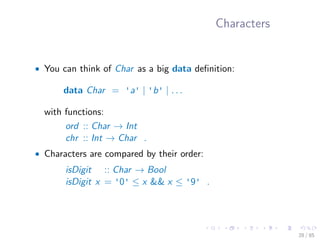
• While (++) repeatedly applies (:), the function concat
repeatedly calls (++):
concat :: [[a]] → [a]
concat [ ] = [ ]
concat (xs : xss) = xs ++ concat xss .
• E.g. concat [[1, 2], [ ], [3, 4], [5]] = [1, 2, 3, 4, 5].
• Compare with sum.
• Is it always true that sum · concat = sum · map sum?
49 / 85](https://image.slidesharecdn.com/slides-140630030216-phpapp01/85/FLOLAC-14-scm-Functional-Programming-Using-Haskell-56-320.jpg)
![Definition by Induction/Recursion
• Rather than giving commands, in functional programming we
specify values; instead of performing repeated actions, we
define values on inductively defined structures.
• Thus induction (or in general, recursion) is the only “control
structure” we have. (We do identify and abstract over plenty
of patterns of recursion, though.)
• To inductively define a function f on lists, we specify a value
for the base case (f [ ]) and, assuming that f xs has been
computed, consider how to construct f (x : xs) out of f xs.
50 / 85](https://image.slidesharecdn.com/slides-140630030216-phpapp01/85/FLOLAC-14-scm-Functional-Programming-Using-Haskell-57-320.jpg)
![Filter
• filter :: (a → Bool) → [a] → [a].
• e.g. filter even [2, 7, 4, 3] = [2, 4]
• filter (λn → n ‘mod‘ 3 == 0) [3, 2, 6, 7] = [3, 6]
• Application: count the number of occurrences of a in a list:
• length · filter ('a' ==)
• Or length · filter (λx → 'a' == x)
51 / 85](https://image.slidesharecdn.com/slides-140630030216-phpapp01/85/FLOLAC-14-scm-Functional-Programming-Using-Haskell-58-320.jpg)
![Filter
• filter p xs keeps only those elements in xs that satisfy p.
filter :: (a → Bool) → [a] → [a]
filter p [ ] = [ ]
filter p (x : xs) | p x = x : filter p xs
| otherwise = filter p xs .
52 / 85](https://image.slidesharecdn.com/slides-140630030216-phpapp01/85/FLOLAC-14-scm-Functional-Programming-Using-Haskell-59-320.jpg)
![List Reversal
• reverse [1, 2, 3, 4] = [4, 3, 2, 1].
reverse :: [a] → [a]
reverse [ ] = [ ]
reverse (x : xs) = reverse xs ++[x] .
53 / 85](https://image.slidesharecdn.com/slides-140630030216-phpapp01/85/FLOLAC-14-scm-Functional-Programming-Using-Haskell-60-320.jpg)
![Map
• map :: (a → b) → [a] → [b] applies the given function to each
element of the input list, forming a new list.
• For example, map (1+) [1, 2, 3, 4, 5] = [2, 3, 4, 5, 6].
• map square [1, 2, 3, 4] = [1, 4, 9, 16].
• How do you define map inductively?
54 / 85](https://image.slidesharecdn.com/slides-140630030216-phpapp01/85/FLOLAC-14-scm-Functional-Programming-Using-Haskell-61-320.jpg)
![Map
• Observe that given f :: (a → b), map f is a function, of type
[a] → [b], that can be defined inductively on lists.
map :: (a → b) → ([a] → [b])
map f [ ] = [ ]
map f (x : xs) = f x : map f xs .
55 / 85](https://image.slidesharecdn.com/slides-140630030216-phpapp01/85/FLOLAC-14-scm-Functional-Programming-Using-Haskell-62-320.jpg)
![Some More About Map
• Every once in a while you may need a small function which
you do not want to give a name to. At such moments you can
use the λ notation:
• map (λx → x × x) [1, 2, 3, 4] = [1, 4, 9, 16]
• Note: a list comprehension can always be translated into a
combination of primitive list generators and map, filter, and
concat.
56 / 85](https://image.slidesharecdn.com/slides-140630030216-phpapp01/85/FLOLAC-14-scm-Functional-Programming-Using-Haskell-63-320.jpg)
![TakeWhile
• takeWhile p xs yields the longest prefix of xs such that p
holds for each element.
• E.g. takeWhile even [2, 4, 5, 6, 8] = [2, 4].
57 / 85](https://image.slidesharecdn.com/slides-140630030216-phpapp01/85/FLOLAC-14-scm-Functional-Programming-Using-Haskell-64-320.jpg)
![TakeWhile
• takeWhile p xs yields the longest prefix of xs such that p
holds for each element.
• E.g. takeWhile even [2, 4, 5, 6, 8] = [2, 4].
• Inductive definition:
takeWhile :: (a → Bool) → [a] → [a]
takeWhile p [ ] = [ ]
takeWhile p (x : xs)
| p x = x : takeWhile p xs
| otherwise = [ ] .
57 / 85](https://image.slidesharecdn.com/slides-140630030216-phpapp01/85/FLOLAC-14-scm-Functional-Programming-Using-Haskell-65-320.jpg)
![DropWhile
• dropWhile p xs drops the prefix from xs.
• E.g. dropWhile even [2, 4, 5, 6, 8] = [5, 6, 8].
• Property: takeWhile p xs ++ dropWhile p xs = xs.
58 / 85](https://image.slidesharecdn.com/slides-140630030216-phpapp01/85/FLOLAC-14-scm-Functional-Programming-Using-Haskell-66-320.jpg)
![DropWhile
• dropWhile p xs drops the prefix from xs.
• E.g. dropWhile even [2, 4, 5, 6, 8] = [5, 6, 8].
• Inductive definition:
dropWhile :: (a → Bool) → [a] → [a]
dropWhile p [ ] = [ ]
dropWhile p (x : xs)
| p x = dropWhile p xs
| otherwise = x : xs .
• Property: takeWhile p xs ++ dropWhile p xs = xs.
58 / 85](https://image.slidesharecdn.com/slides-140630030216-phpapp01/85/FLOLAC-14-scm-Functional-Programming-Using-Haskell-67-320.jpg)
![All Prefixes and Suffixes
• inits [1, 2, 3] = [[ ], [1], [1, 2], [1, 2, 3]]
inits :: [a] → [[a]]
inits [ ] = [[ ]]
inits (x : xs) = [ ] : map (x :) (inits xs) .
• tails [1, 2, 3] = [[1, 2, 3], [2, 3], [3], [ ]]
tails :: [a] → [[a]]
tails [ ] = [[ ]]
tails (x : xs) = (x : xs) : tails xs .
59 / 85](https://image.slidesharecdn.com/slides-140630030216-phpapp01/85/FLOLAC-14-scm-Functional-Programming-Using-Haskell-68-320.jpg)
![Totality
• Structure of our definitions so far:
f [ ] = . . .
f (x : xs) = . . . f xs . . .
• Both the empty and the non-empty cases are covered,
guaranteeing there is a matching clause for all inputs.
• The recursive call is made on a “smaller” argument,
guranteeing termination.
• Together they guarantee that every input is mapped to some
output. Thus they define total functions on lists.
60 / 85](https://image.slidesharecdn.com/slides-140630030216-phpapp01/85/FLOLAC-14-scm-Functional-Programming-Using-Haskell-69-320.jpg)
![Take and Drop
• take n takes the first n elements of the list.
• For example, take 0 xs = [],
• take 3 "abcde" = "abc",
• take 3 "ab" = "ab".
• Dually, drop n drops the first n elements of the list.
• For example, drop 0 xs = xs,
• drop 3 "abcde" = "cd",
• drop 3 "ab" = "".
• take n xs ++ drop n xs = xs, as long as evaluation of n
terminates.
66 / 85](https://image.slidesharecdn.com/slides-140630030216-phpapp01/85/FLOLAC-14-scm-Functional-Programming-Using-Haskell-75-320.jpg)
![Take and Drop
• They can be defined by induction on the first argument:
take :: N → [a] → [a]
take 0 xs = [ ]
take (1+ n) [ ] = [ ]
take (1+ n) (x : xs) = x : take n xs .
•
drop :: N → [a] → [a]
drop 0 xs = xs
drop (1+ n) [ ] = [ ]
drop (1+ n) (x : xs) = drop n xs .
• Note: take n xs ++ drop n xs = xs, for all n and xs.
67 / 85](https://image.slidesharecdn.com/slides-140630030216-phpapp01/85/FLOLAC-14-scm-Functional-Programming-Using-Haskell-76-320.jpg)
![• Some functions make more sense when it is defined only on
non-empty lists:
f [x] = . . .
f (x : xs) = . . .
• What about totality?
• They are in fact functions defined on a different datatype:
data [a]+
= Singleton a | a : [a]+
.
• We do not want to define map, filter again for [a]+
. Thus we
reuse [a] and pretend that we were talking about [a]+
.
• It’s the same with N. We embedded N into Int.
• Ideally we’d like to have some form of subtyping. But that
makes the type system more complex.
69 / 85](https://image.slidesharecdn.com/slides-140630030216-phpapp01/85/FLOLAC-14-scm-Functional-Programming-Using-Haskell-78-320.jpg)
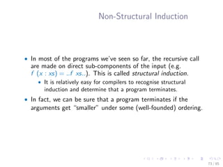
![Lexicographic Induction
• It also occurs often that we perform lexicographic induction
on multiple arguments: some arguments decrease in size,
while others stay the same.
• E.g. the function merge merges two sorted lists into one
sorted list:
merge :: [Int] → [Int] → [Int]
merge [ ] [ ] = [ ]
merge [ ] (y : ys) = y : ys
merge (x : xs) [ ] = x : xs
merge (x : xs) (y : ys)
| x ≤ y = x : merge xs (y : ys)
| otherwise = y : merge (x : xs) ys .
70 / 85](https://image.slidesharecdn.com/slides-140630030216-phpapp01/85/FLOLAC-14-scm-Functional-Programming-Using-Haskell-79-320.jpg)
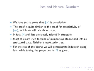
![Zip
• zip :: [a] → [b] → [(a, b)]
• e.g. zip "abcde" [1, 2, 3] = [('a', 1), ('b', 2), ('c', 3)]
• The length of the resulting list is the length of the shorter
input list.
71 / 85](https://image.slidesharecdn.com/slides-140630030216-phpapp01/85/FLOLAC-14-scm-Functional-Programming-Using-Haskell-80-320.jpg)
![Zip
zip :: [a] → [b] → [(a, b)]
zip [ ] [ ] = [ ]
zip [ ] (y : ys) = [ ]
zip (x : xs) [ ] = [ ]
zip (x : xs) (y : ys) = (x, y) : zip xs ys .
72 / 85](https://image.slidesharecdn.com/slides-140630030216-phpapp01/85/FLOLAC-14-scm-Functional-Programming-Using-Haskell-81-320.jpg)
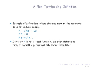
![Mergesort
• In the implemenation of mergesort below, for example, the
arguments always get smaller in size.
msort :: [Int] → [Int]
msort [ ] = [ ]
msort [x] = [x]
msort xs = merge (msort ys) (msort zs) ,
where n = length xs ‘div‘ 2
ys = take n xs
zs = drop n xs .
• What if we omit the case for [x]?
• If all cases are covered, and all recursive calls are applied to
smaller arguments, the program defines a total function.
74 / 85](https://image.slidesharecdn.com/slides-140630030216-phpapp01/85/FLOLAC-14-scm-Functional-Programming-Using-Haskell-83-320.jpg)
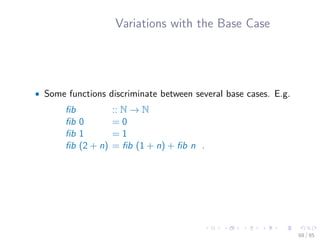
![A Common Pattern We’ve Seen Many
Times. . .
• Many programs we have seen follow a similar pattern:
sum [ ] = 0
sum (x : xs) = x + sum xs .
length [ ] = 0
length (x : xs) = 1 + length xs .
map f [ ] = [ ]
map f (x : xs) = f x : map f xs .
• This pattern is extracted and called foldr:
foldr f e [ ] = e
foldr f e (x : xs) = f x (foldr f e xs) .
76 / 85](https://image.slidesharecdn.com/slides-140630030216-phpapp01/85/FLOLAC-14-scm-Functional-Programming-Using-Haskell-85-320.jpg)
![Replacing Constructors
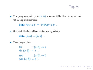
• The function foldr is among the most important functions on
lists.
foldr :: (a → b → b) → b → [a] → b
• One way to look at foldr (⊕) e is that it replaces [ ] with e
and (:) with (⊕):
foldr (⊕) e [1, 2, 3, 4]
= foldr (⊕) e (1 : (2 : (3 : (4 : [ ]))))
= 1 ⊕ (2 ⊕ (3 ⊕ (4 ⊕ e))).
• sum = foldr (+) 0.
• One can see that id = foldr (:) [ ].
77 / 85](https://image.slidesharecdn.com/slides-140630030216-phpapp01/85/FLOLAC-14-scm-Functional-Programming-Using-Haskell-86-320.jpg)
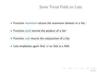
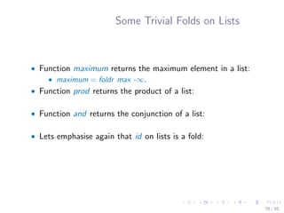
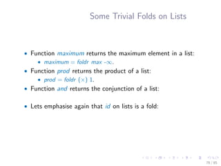
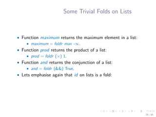
![Some Trivial Folds on Lists
• Function maximum returns the maximum element in a list:
• maximum = foldr max -∞.
• Function prod returns the product of a list:
• prod = foldr (×) 1.
• Function and returns the conjunction of a list:
• and = foldr (&&) True.
• Lets emphasise again that id on lists is a fold:
• id = foldr (:) [ ].
78 / 85](https://image.slidesharecdn.com/slides-140630030216-phpapp01/85/FLOLAC-14-scm-Functional-Programming-Using-Haskell-91-320.jpg)
![Some Slightly Complex Folds
• length = foldr (λx n → 1 + n) 0.
• map f = foldr (λx xs → f x : xs) [ ].
• xs ++ ys = foldr (:) ys xs. Compare this with id!
• filter p = foldr (fil p) [ ]
where fil p x xs = if p x then (x : xs) else xs.
79 / 85](https://image.slidesharecdn.com/slides-140630030216-phpapp01/85/FLOLAC-14-scm-Functional-Programming-Using-Haskell-92-320.jpg)

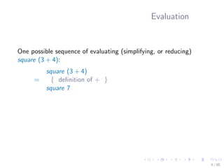
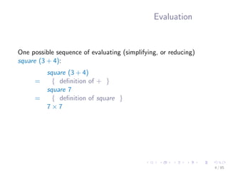
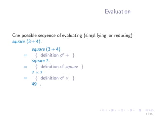
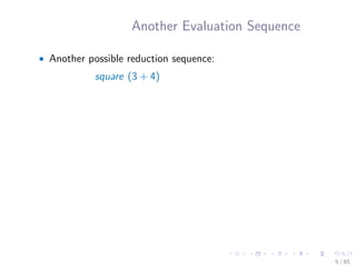
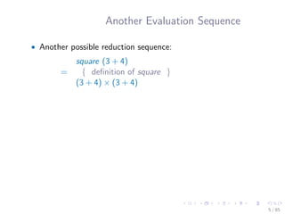
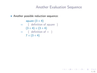
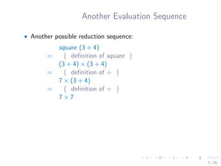
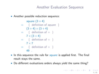
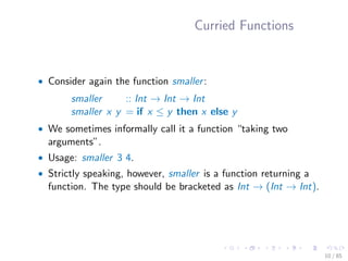
This document provides an introduction to functional programming concepts in Haskell, including: - Defining functions and evaluating expressions through reduction sequences. - Currying and partial application of functions. - Pattern matching and defining functions through multiple cases.


![[FT-8][banacorn] Socket.IO for Haskell Folks](https://cdn.slidesharecdn.com/ss_thumbnails/ft-140421081017-phpapp02-thumbnail.jpg?width=640&height=640&fit=bounds)


![[FT-11][ltchen] A Tale of Two Monads](https://cdn.slidesharecdn.com/ss_thumbnails/monads-140308101321-phpapp01-140421092116-phpapp01-thumbnail.jpg?width=640&height=640&fit=bounds)