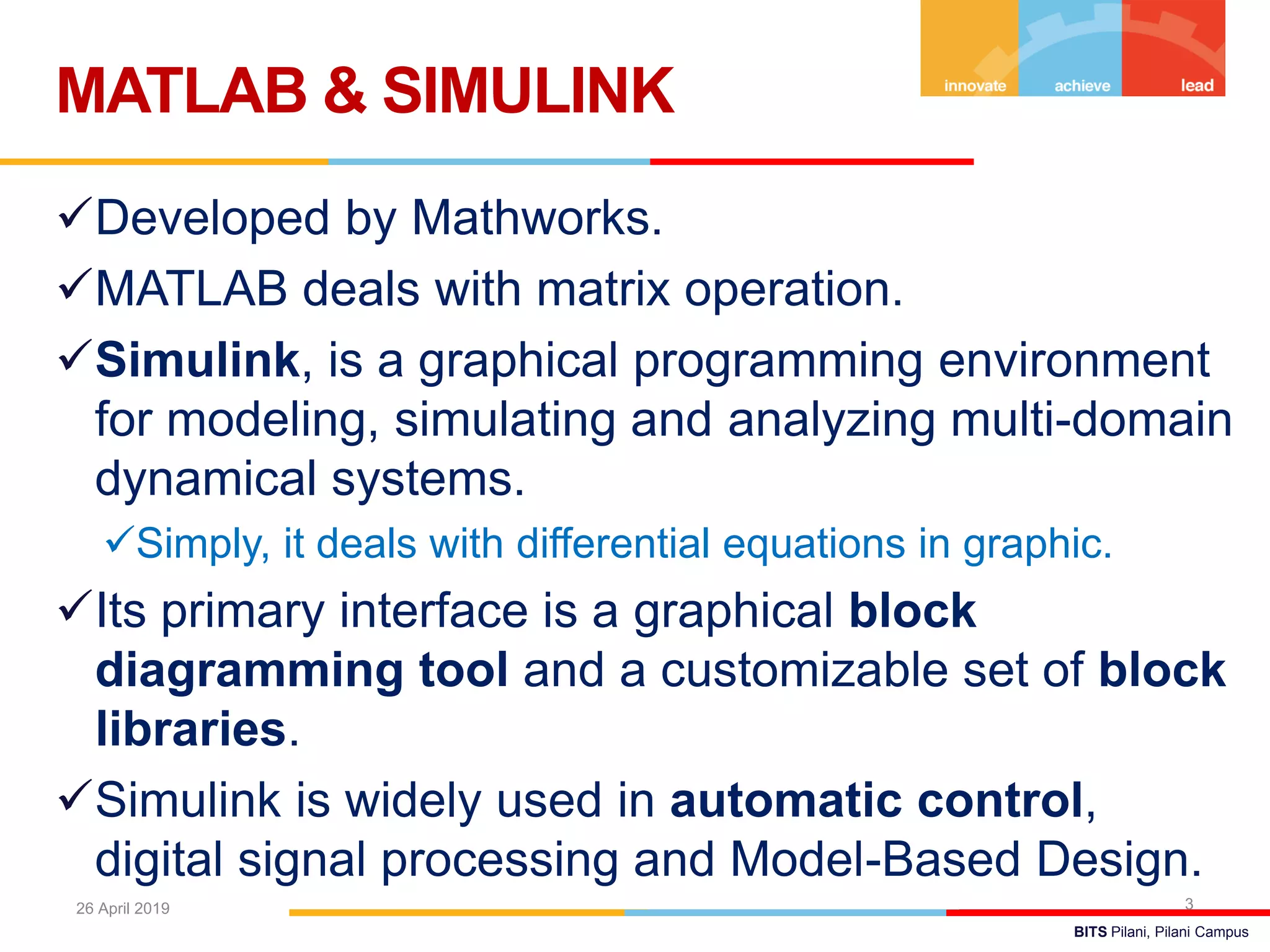
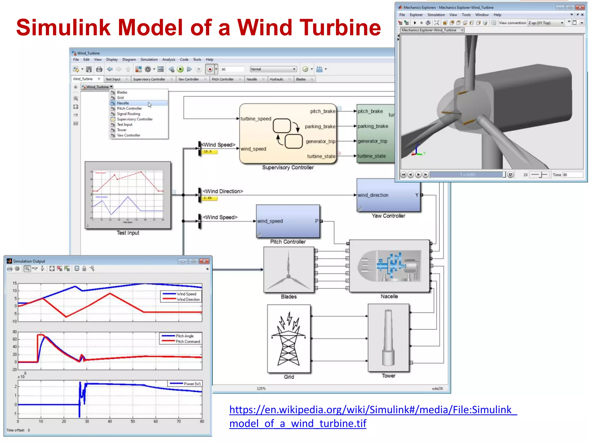
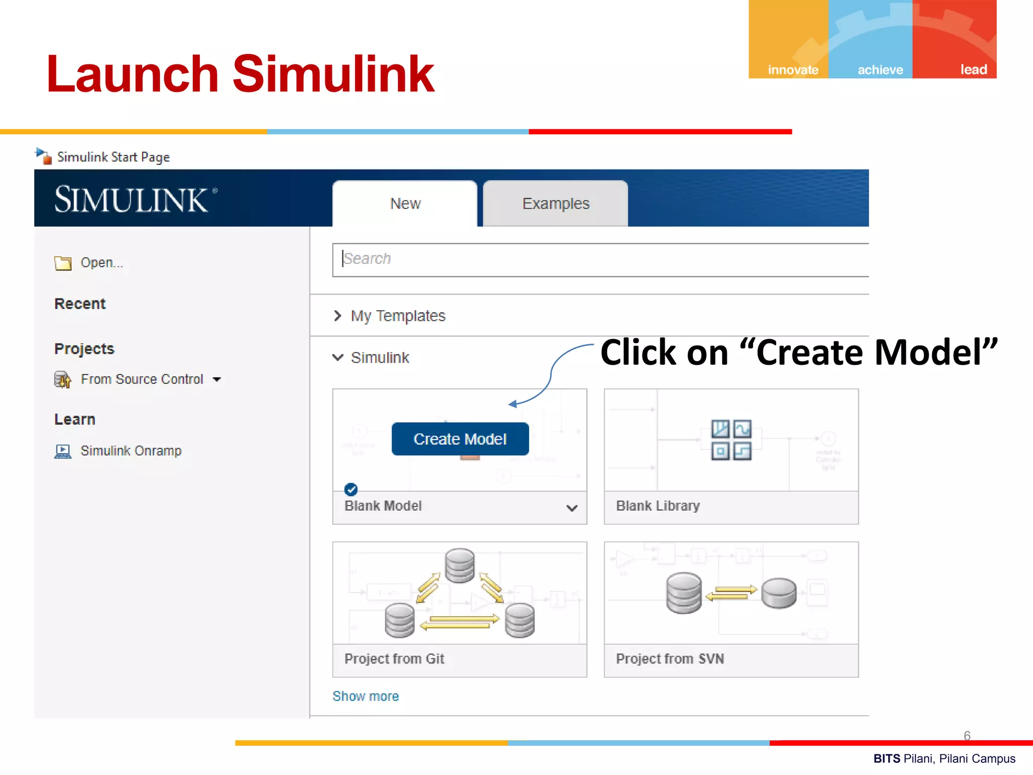
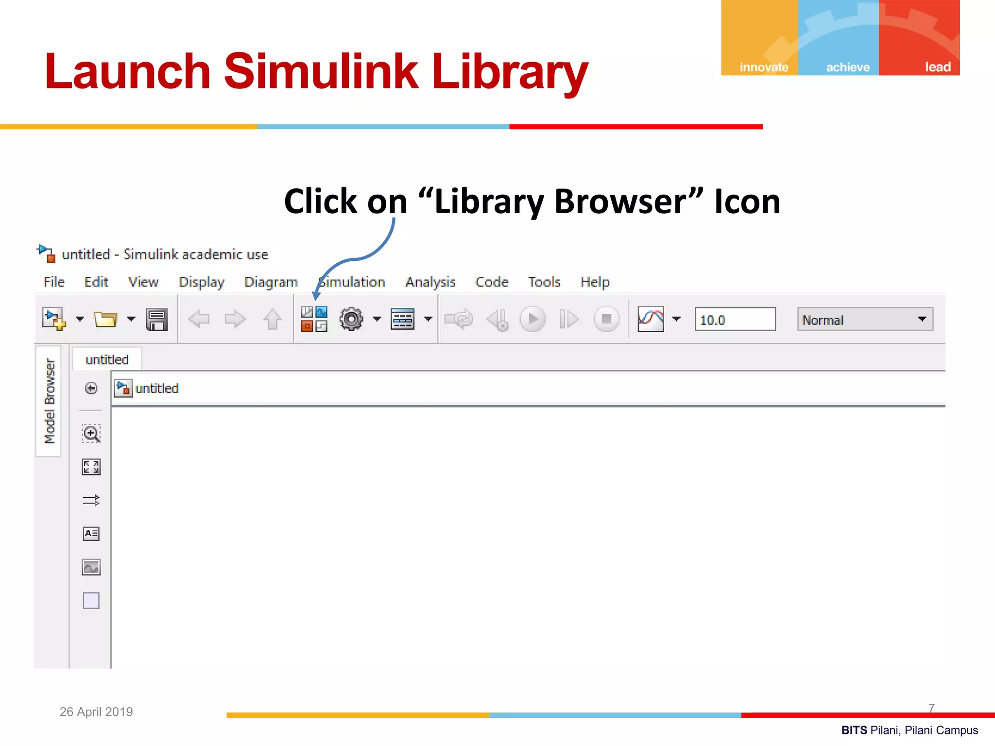
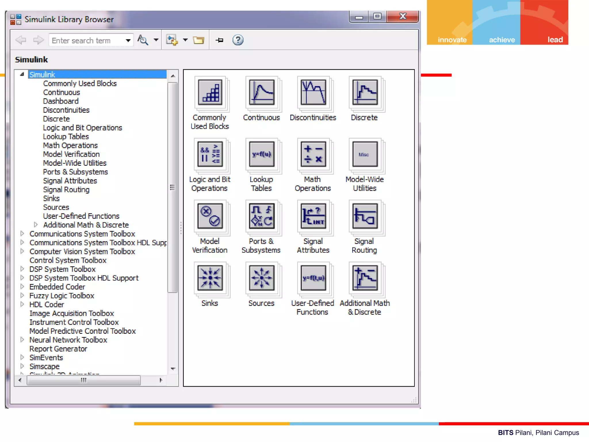
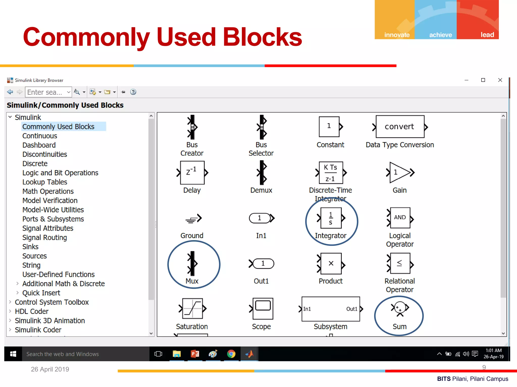
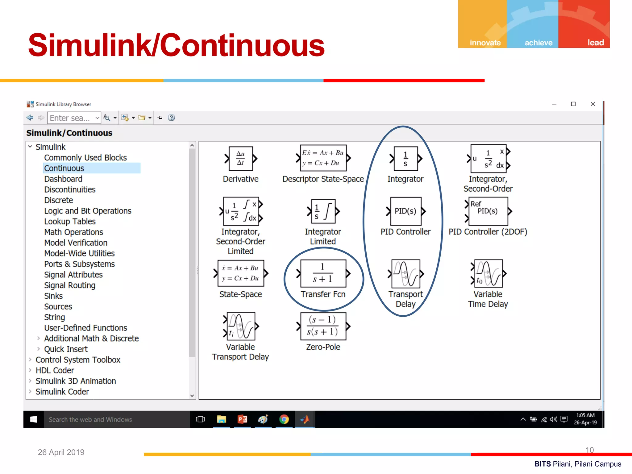
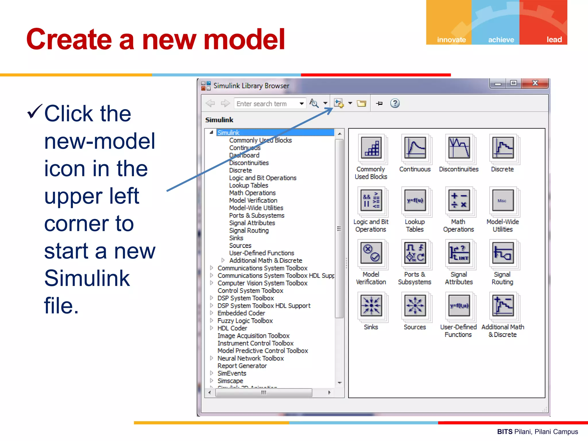
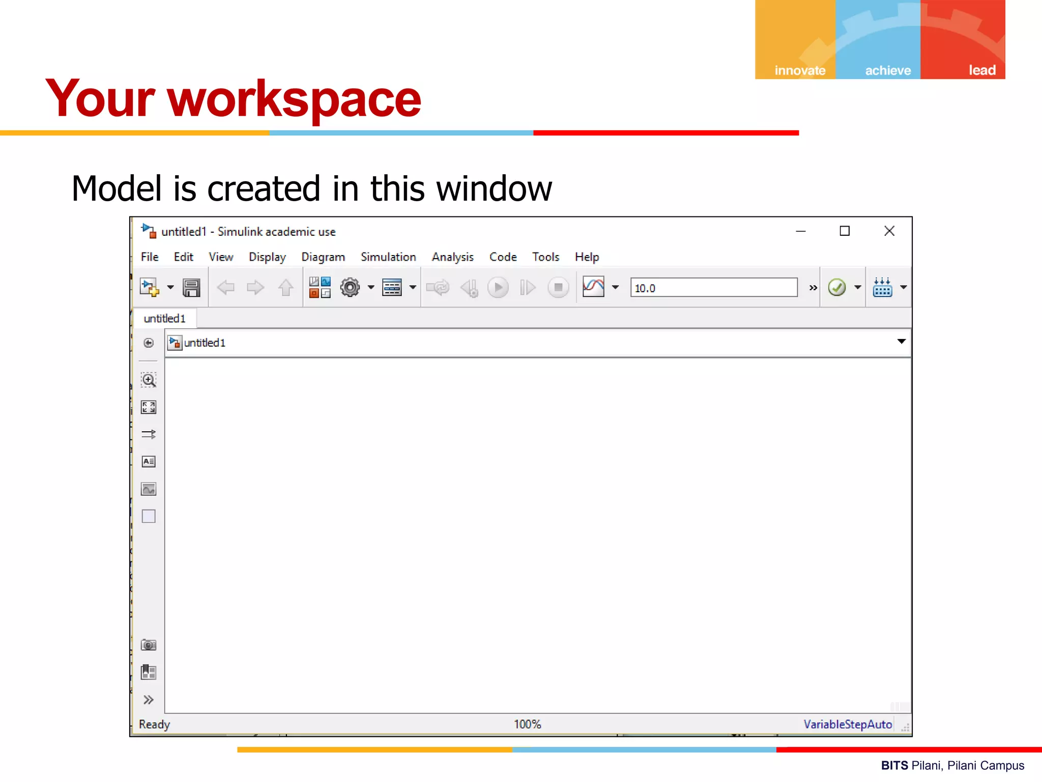
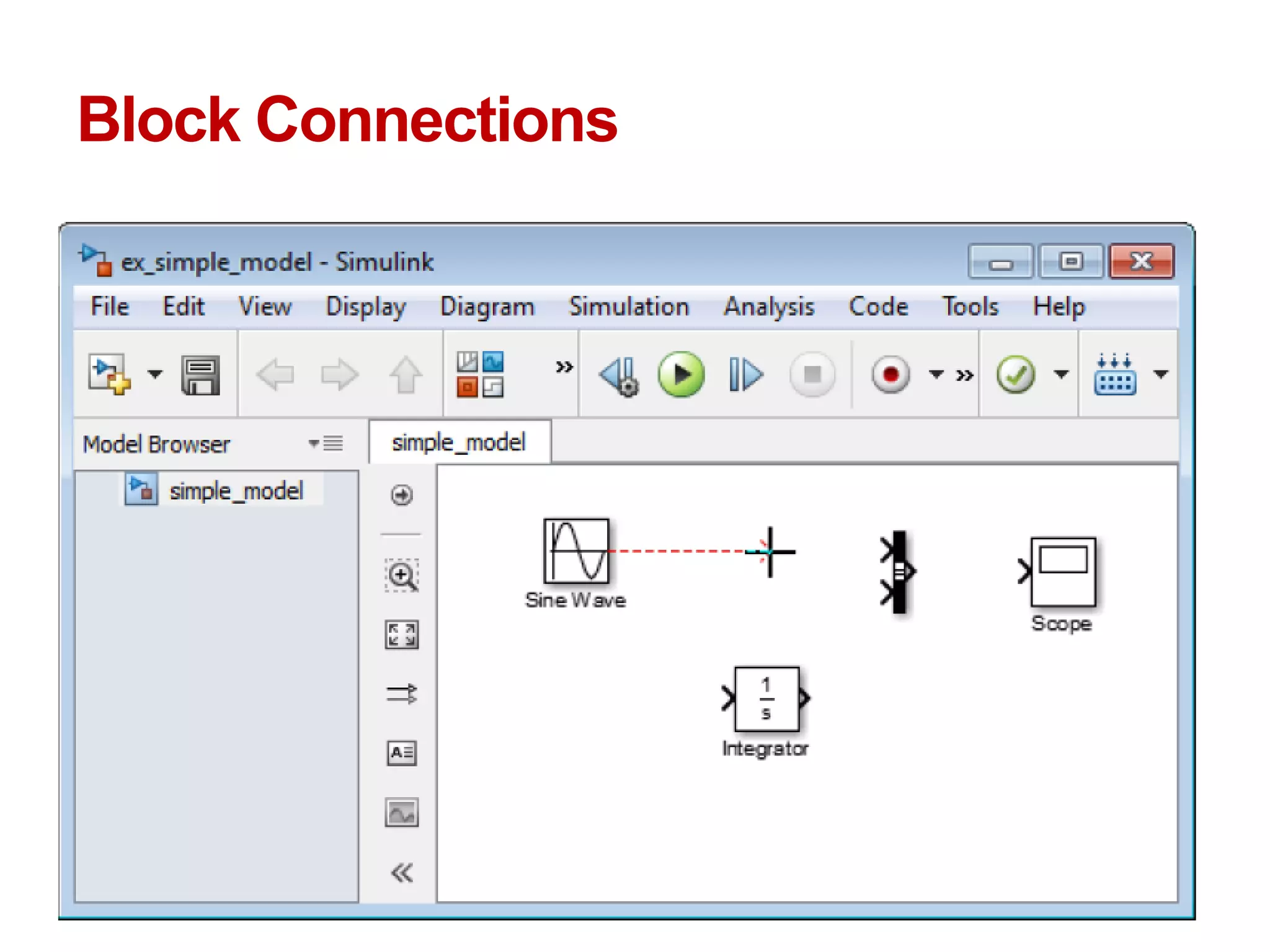
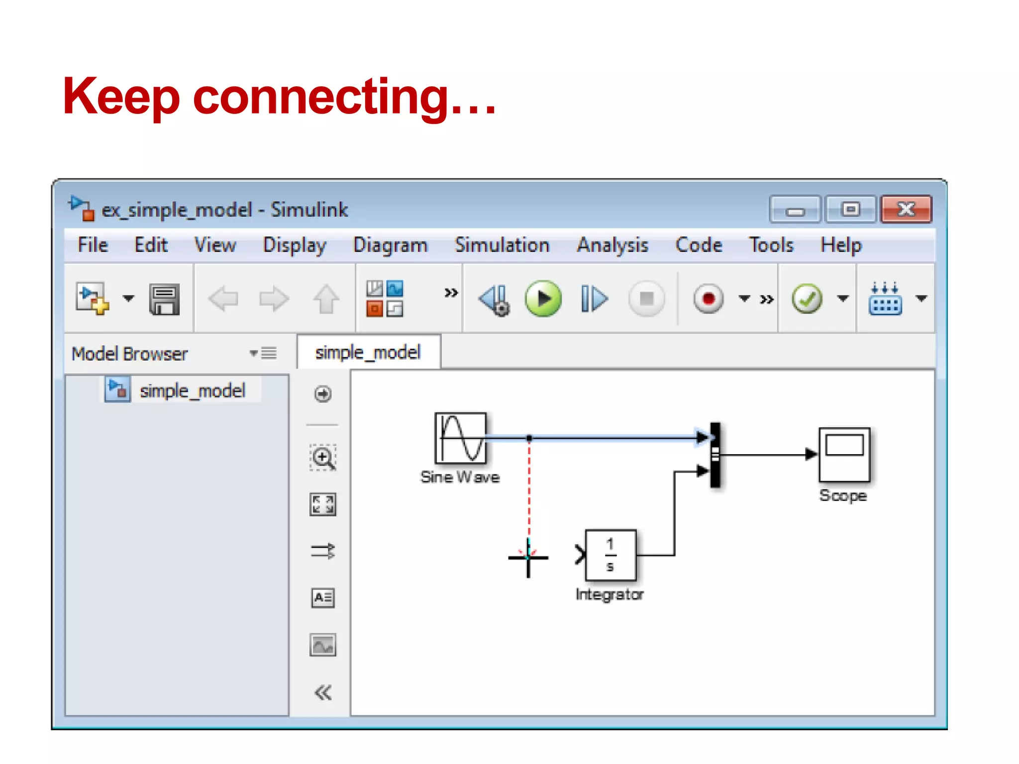
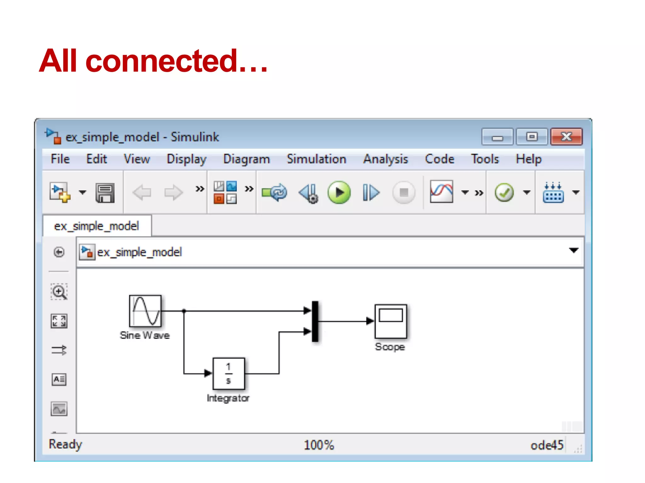
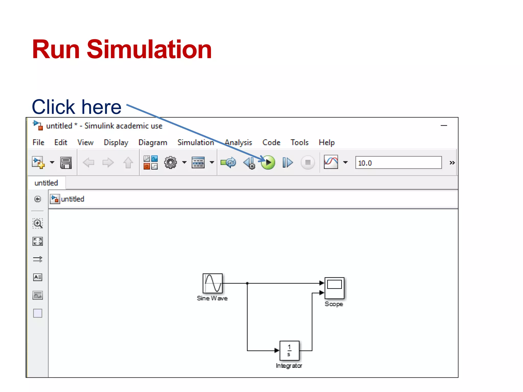
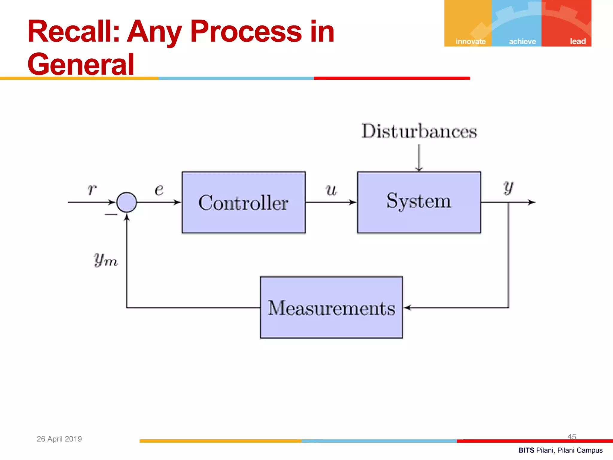
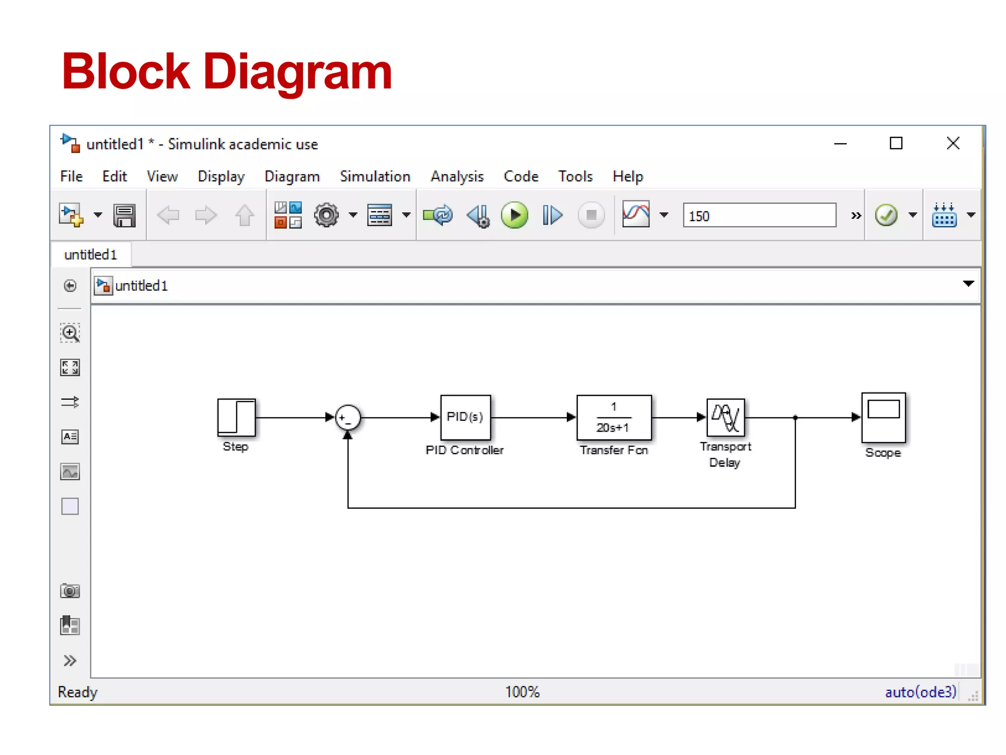
The document describes a presentation on using MATLAB and Simulink for process engineering. It discusses how Simulink can be used to model, simulate, and analyze multi-domain dynamic systems using graphical block diagrams. Examples are provided on building simple models in Simulink, including integrating a sine wave and modeling a first-order process. Process control applications are demonstrated, such as modeling different types of controllers and their effects.

1. BITS Pilani
Pilani Campus
MATLAB & SIMULINK
for Process Engineers
@
SLIET, LONGOWAL
under TEQIP-3, April 25-26, 2019

2. BITS Pilani
Pilani Campus
Amit Jain, PhD
Assistant Professor
Dept. of Chemical Engg.
BITS Pilani – Pilani Campus

3. BITS Pilani, Pilani Campus
Developed by Mathworks.
MATLAB deals with matrix operation.
Simulink, is a graphical programming environment
for modeling, simulating and analyzing multi-domain
dynamical systems.
Simply, it deals with differential equations in graphic.
Its primary interface is a graphical block
diagramming tool and a customizable set of block
libraries.
Simulink is widely used in automatic control,
digital signal processing and Model-Based Design.
MATLAB & SIMULINK
326 April 2019

4. BITS Pilani, Pilani Campus
Model based design of control systems.
Simulink Applications
426 April 2019
Simulink Model of a Wind Turbine
https://en.wikipedia.org/wiki/Simulink#/media/File:Simulink_
model_of_a_wind_turbine.tif

5. BITS Pilani, Pilani Campus
First launch MATLAB by double clicking the
icon on desktop.
Click on the Simulink Library/Simulink
Alternate launch: at command prompt >> type
simulink and press  Enter
Launch Simulink

6. BITS Pilani, Pilani Campus
Launch Simulink
6
Click on “Create Model”

7. BITS Pilani, Pilani Campus
Launch Simulink Library
726 April 2019
Click on “Library Browser” Icon

8. BITS Pilani, Pilani Campus

9. BITS Pilani, Pilani Campus
Commonly Used Blocks
926 April 2019

10. BITS Pilani, Pilani Campus
Simulink/Continuous
1026 April 2019

11. BITS Pilani, Pilani Campus
Click the
new-model
icon in the
upper left
corner to
start a new
Simulink
file.
Create a new model

12. BITS Pilani, Pilani Campus
Your workspace
Model is created in this window

13. BITS Pilani, Pilani Campus
 Simulating this model integrates a sine wave signal to a
cosine signal and then displays the result, along with the
original signal, in a Scope window.
Simple Simulink Model

14. Add Blocks to Model
Drag the
Sine Wave
block to the
Simulink
Editor.

15. Add other blocks too…

16. Move the blocks as per convenience

17. Block Connections

18. Keep connecting…

19. All connected…

20. Define Configuration Parameters

21. Run Simulation
Click here

22. Results: Double click scope block

23. Save the file

24. Example 1: a simple model
Build a Simulink model that solves the
differential equation
Initial condition
First, sketch a simulation diagram of this
mathematical model (equation) (3 min.)
 tx 2sin3
.1)0( x

25. Simulation diagram
Input is the forcing function 3sin(2t)
Output is the solution of the differential equation
x(t)
Now build this model in Simulink
xx
s
1
3sin(2t)
(input)
x(t)
(output)
1)0( x
integrator

26. Select an input block
Drag a Sine Wave block
from the Sources library
to the model window

27. Select an operator block
Drag an Integrator block
from the Continuous library
to the model window

28. Select an output block
Drag a Scope block from the
Sinks library to the model
window

29. Connect blocks with signals
Place your cursor on
the output port (>) of
the Sine Wave block
Drag from the Sine
Wave output to the
Integrator input
Drag from the
Integrator output to
the Scope input
Arrows indicate the
direction of the signal flow.

30. Select simulation parameters
Double-click on
the Sine Wave
block to set
amplitude = 3
and freq = 2.
This produces the
desired input of
3sin(2t)

31. Select simulation parameters
Double-click on
the Integrator
block to set
initial condition
= -1.
This sets our IC
x(0) = -1.

32. Select simulation parameters
Double-click on
the Scope to view
the simulation
results

33. Run the simulation
In the model
window, from the
Simulation pull-
down menu,
select Start
View the output
x(t) in the Scope
window.

34. BITS Pilani, Pilani Campus
Simulation Results
To verify that this
plot represents the
solution to the
problem, solve the
equation analytically.
The analytical result,
matches the plot
(the simulation
result) exactly.
 ttx 2cos)( 2
3
2
1


35. BITS Pilani, Pilani Campus
Any Process in General
3526 April 2019

36. BITS Pilani, Pilani Campus
Process Control Example
3626 April 2019

37. BITS Pilani, Pilani Campus
Servo Problem or Servo mechanism or Set point
tracking
• Set point changes but there is no change in the Load
or DV
Regulator Problem
• Load changes but there is no change in set point
Servo Problem Versus Regulator
Problem
3726 April 2019

38. BITS Pilani, Pilani Campus
Typical Response of
Feedback Control Systems
3826 April 2019

39. BITS Pilani, Pilani Campus
Effect of Kc in P-Only Control
3926 April 2019

40. BITS Pilani, Pilani Campus
Effect of Kc and TI in PI
Control
4026 April 2019

41. BITS Pilani, Pilani Campus
Effect of Derivative Time in
PID Control
4126 April 2019
Brings stabilizing effect by
reducing the number of
oscillations.

42. BITS Pilani, Pilani Campus
PID Controller Block Diagram
4226 April 2019

43. BITS Pilani, Pilani Campus
Simulink Application to
Process Control
Consider the standard first-order-plus-time-delay
model,
Chapter12
 
  parameter)SimulinkD&I(P,
or
1
1
Ds
s
I
PsG
sk
s
k
ks
s
ksG
c
Dc
I
c
cD
I
cc













 



The controller transfer function model:

44. Example-1

45. BITS Pilani, Pilani Campus
Recall: Any Process in
General
4526 April 2019

46. BITS Pilani, Pilani Campus
Standard Block Diagram of a
Feedback Control System
4626 April 2019

47. Block Diagram

48. Process with disturbance variable

49. Example-2 second order process
  15110
2



ss
e
GG
s
d

50. Results

51. Thank you