
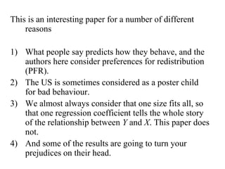
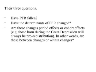
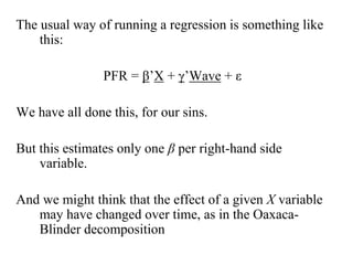
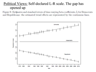
![There is a lot of variability, but the trend line is almost
flat.
[Would have been nice to see this figure overlaid with
red and blue to denote Democratic and Republican
Presidencies]
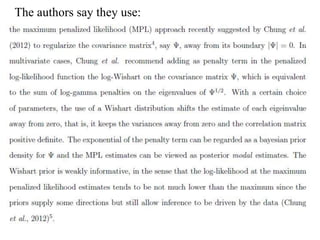
Model PFR with the following right-hand side variables:
household equivalent income, age, gender, marital
status, children at home, race, years of education,
labour-force status, past experience of
unemployment in the last ten years, religious
denomination, religious attendance, and political
views](https://image.slidesharecdn.com/wk5vmjmsuosqkcenygbg-signature-564f90475daa5093001dd9a9e6b11ee7cdc49adae3c069ed47cd6a065c631606-poli-140830074918-phpapp02/85/Session-8-a-clark-discussionzellipittau-9-320.jpg)
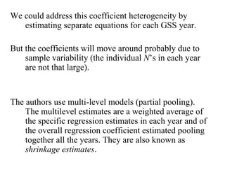

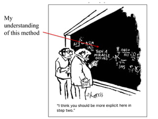
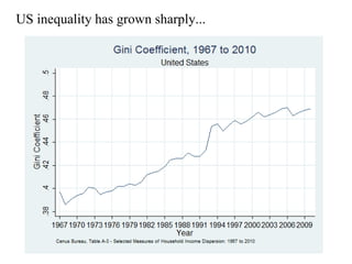
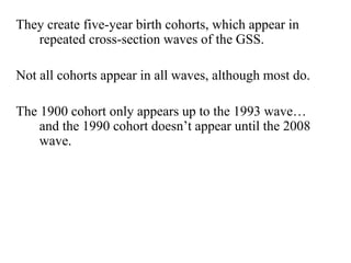
![Which variables are P (time-varying coefficients) and
which R?
Estimate separately by year and see which of the
estimated β’s are small and don’t change
[But isn’t this the procedure that you criticised in the
first place?]
R = marital status, gender, religion, religious practice,
labour-force status, previous unemployment.](https://image.slidesharecdn.com/wk5vmjmsuosqkcenygbg-signature-564f90475daa5093001dd9a9e6b11ee7cdc49adae3c069ed47cd6a065c631606-poli-140830074918-phpapp02/85/Session-8-a-clark-discussionzellipittau-17-320.jpg)
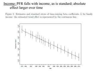
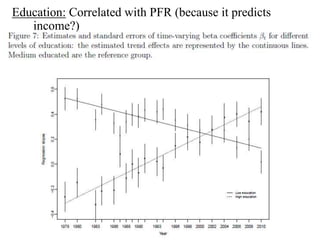
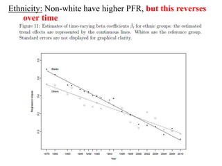
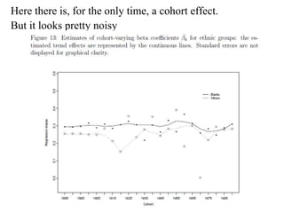

This paper analyzes how attitudes toward redistribution in the US have changed over time from 1972 to 2010 using data from the General Social Survey. The authors find that while overall support for redistribution has remained flat, the determinants of those attitudes have changed significantly. Younger people and those with lower incomes or less education now support redistribution more, while the attitudes of older people and those with higher incomes or more education have become more polarized. Non-white groups also showed higher support for redistribution, but this difference has decreased over time. These results suggest preferences around redistribution in the US have become more stratified along socioeconomic lines in recent decades.


![Session 7 b commentson daneilkerpaperonukr&d servicelives2014iariw[1]](https://cdn.slidesharecdn.com/ss_thumbnails/pwfpecwntsmdld64j1xg-signature-6de5ee34a7e0a8be608105cfc95b1f55459403214875a488c94e063931d3b0c1-poli-140830080216-phpapp01-thumbnail.jpg?width=640&height=640&fit=bounds)


