1) The document discusses estimation and sample size determination for finite populations, specifically for estimating the mean and proportion. It describes how to calculate confidence intervals and determine sample sizes when sampling without replacement using the finite population correction factor. 2) Formulas are provided for confidence intervals for the mean and proportion when sampling from a finite population without replacement. The finite population correction factor adjusts the standard error and sample size calculations. 3) Examples are given to illustrate how to set up confidence intervals for the mean and proportion and how to determine the necessary sample size using the finite population correction factor.

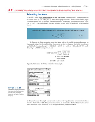
1. 8.7: Estimation and Sample Size Determination for Finite Populations CD8-1
8.7: ESTIMATION AND SAMPLE SIZE DETERMINATION FOR FINITE POPULATIONS
Estimating the Mean
In section 7.3 the finite population correction (fpc) factor is used to reduce the standard error
by a value equal to (N − n )/(N − 1) . When developing confidence interval estimates for popu-
lation parameters, the fpc factor is used when samples are selected without replacement. Thus,
the (1 Ϫ ␣) × 100% confidence interval estimate for the mean is calculated as in Equation
(8.12).
CONFIDENCE INTERVAL FOR A MEAN (σ UNKNOWN) FOR A FINITE POPULATION
S N −n
X ± t n −1 (8.12)
n N −1
To illustrate the finite population correction factor, refer to the confidence interval estimate for
the mean developed for Saxon Plumbing Company in section 8.2. Suppose that in this month there
are 5,000 sales invoices. Using X = $110.27, S = $28.95, N = 5,000, n = 100, and with 95% confi-
dence, t99 = 1.9842. From equation (8.12)
5,000 − 100
28.95
110.27 ± (1.9842)
100 5,000 − 1
= 110.27 ± 5.744(0.99)
110.27 ± 5.69
$104.58 ≤ µ ≤ $115.96
Figure 8.29 illustrates the PHStat output for this example.
FIGURE 8.29
Confidence interval estimate for
the mean sales invoice amount
with the finite population
correction for Saxon Plumbing
Company
In this case, because the sample is a very small fraction of the population, the correction factor has a
minimal effect on the width of the confidence interval. To examine the effect of the correction factor
when the sample size is more than 5% of the population size, see Example 8.10.

2. CD8-2 CD MATERIAL
Example 8.10 In Example 8.3, a sample of 30 insulators was selected. Suppose a population of 300 insulators were
produced by the company. Set up a 95% confidence interval estimate of the population mean.
ESTIMATING THE MEAN FORCE
FOR INSULATORS SOLUTION Using the finite population correction factor, with X = 1,723.4 pounds, S = 89.55,
n = 30, N = 300, and t29 = 2.0452 (for 95% confidence):
S N −n
X ± t n −1
n N −1
89.55 300 − 30
= 1,723.4 ± (2.0452)
30 300 − 1
= 1,723.4 ± 33.44(0.9503)
= 1,723.4 ± 31.776
1,691.62 ≤ µ ≤ 1,755.18
Here, because 10% of the population is to be sampled, the fpc factor has a small effect on the confi-
dence interval estimate.
Estimating the Proportion
In sampling without replacement, the (1 Ϫ ␣) × 100% confidence interval estimate of the propor-
tion is defined in Equation (8.13).
CONFIDENCE INTERVAL ESTIMATE FOR THE PROPORTION USING THE FINITE
POPULATION CORRECTION FACTOR
ps (1 − ps ) N − n
ps ± Z (8.13)
n N −1
To illustrate the use of the finite population correction factor when developing a confidence interval
estimate of the population proportion, consider again the estimate developed for Saxon Home
Improvement Company in section 8.3. For these data, N = 5,000, n = 100, ps = 10/100 = 0.10, and
with 95% confidence, Z = 1.96. Using Equation (8.13),
ps (1 − ps ) N − n
ps ± Z
n N −1
(0.10)(0.90) 5,000 − 100
= 0.10 ± (1.96)
100 5,000 − 1
= 0.10 ± (1.96)(0.03)(0.99)
= 0.10 ± .0582
0.0418 ≤ p ≤ 0.1582
In this case, because the sample is a very small fraction of the population, the fpc factor has virtually
no effect on the confidence interval estimate.

3. 8.7: Estimation and Sample Size Determination for Finite Populations CD8-3
Determining the Sample Size
Just as the fpc factor is used to develop confidence interval estimates, it also is used to determine
sample size when sampling without replacement. For example, in estimating the mean, the sampling
error is
σ N −n
e =Z
n N −1
and in estimating the proportion, the sampling error is
p (1 − p ) N − n
e =Z
n N −1
To determine the sample size in estimating the mean or the proportion from Equations (8.4) and (8.5),
Z 2 σ2 Z 2 p (1 − p )
n0 = and n0 =
e2 e2
where n0 is the sample size without considering the finite population correction factor. Applying the
fpc factor results in the actual sample size n, computed as in Equation (8.14).
SAMPLE SIZE DETERMINATION USING THE FINITE POPULATION CORRECTION FACTOR
n 0N
n = (8.14)
n 0 + (N − 1)
In determining the sample size for Saxon Home Improvement Company, a sample size of 97 was
needed (rounded up from 96.04) for the mean and a sample of 100 (rounded up from 99.96) was
needed for the proportion. Using the fpc factor in Equation (8.14) for the mean, with N = 5,000,
e = $5, S = $25, and Z = 1.96 (for 95% confidence), leads to
(96.04)(5,000)
n = = 94.24
96.04 + (5,000 − 1)
Thus, n = 95.
Using the fpc factor in Equation (8.14) for the proportion, with N = 5,000, e = 0.07, p = 0.15,
and Z = 1.96 (for 95% confidence),
(99.96)(5,000)
n = = 98.02
99.96 + (5,000 − 1)
Thus, n = 99.
To satisfy both requirements simultaneously with one sample, the larger sample size of 99 is
needed. PHStat output is displayed in Figure 8.30.
FIGURE 8.30
Sample size for estimating the
mean sales invoice amount with
the finite population correction
for the Saxon Home
Improvement Company

4. CD8-4 CD MATERIAL
PROBLEMS FOR SECTION 8.7
Learning the Basics depositors who have more than one account at the bank.
What sample size is needed if sampling is done without
8.88 If X = 75, S = 24, n = 36, and N = 200, set up a 95% confi- replacement?
dence interval estimate of the population mean µ if sam- c. What are your answers to (a) and (b) if the bank has
pling is done without replacement. 2,000 depositors?
8.89 Consider a population of 1,000 where the standard deviation 8.93 An automobile dealer wants to estimate the proportion of cus-
is assumed equal to 20. What sample size would be required tomers who still own the cars they purchased 5 years earlier.
if sampling is done without replacement if you desire 95% Sales records indicate that the population of owners is 4,000.
confidence and a sampling error of ±5? a. Set up a 95% confidence interval estimate of the popula-
tion proportion of all customers who still own their cars
Applying the Concepts 5 years after they were purchased if a random sample of
200 customers selected without replacement from the
8.90 The quality control manager at a lightbulb factory needs to automobile dealer’s records indicate that 82 still own cars
estimate the mean life of a large shipment of lightbulbs. The that were purchased 5 years earlier.
process standard deviation is known to be 100 hours. b. What sample size is necessary to estimate the true pro-
Assume that the shipment contains a total of 2,000 light- portion to within ±0.025 with 95% confidence?
bulbs and that sampling is done without replacement. c. What are your answers to (a) and (b) if the population
a. Set up a 95% confidence interval estimate of the popula- consists of 6,000 owners?
tion mean life of lightbulbs in this shipment if a random
8.94 The inspection division of the Lee County Weights and
sample of 50 lightbulbs selected from the shipment indi-
Measures Department is interested in estimating the actual
cates a sample average life of 350 hours.
amount of soft drink that is placed in 2-liter bottles at the
b. Determine the sample size needed to estimate the average
local bottling plant of a large nationally known soft-drink
life to within ±20 hours with 95% confidence.
company. The population consists of 2,000 bottles. The bot-
c. What are your answers to (a) and (b) if the shipment
tling plant has informed the inspection division that the
contains 1,000 lightbulbs?
standard deviation for 2-liter bottles is 0.05 liter.
8.91 A survey is planned to determine the mean annual family a. Set up a 95% confidence interval estimate of the popula-
medical expenses of employees of a large company. The tion mean amount of soft drink per bottle if a random
management of the company wishes to be 95% confident sample of one hundred 2-liter bottles obtained without
that the sample average is correct to within ±$50 of the true replacement from this bottling plant indicates a sample
average annual family medical expenses. A pilot study indi- average of 1.99 liters.
cates that the standard deviation is estimated as $400. How b. Determine the sample size necessary to estimate the pop-
large a sample size is necessary if the company has 3,000 ulation mean amount to within ±0.01 liter with 95%
employees and if sampling is done without replacement? confidence.
c. What are your answers to (a) and (b) if the population
8.92 The manager of a bank that has 1,000 depositors in a small
consists of 1,000 bottles?
city wants to determine the proportion of its depositors with
more than one account at the bank. 8.95 A stationery store wants to estimate the mean retail value of
a. Set up a 90% confidence interval estimate of the popu- greeting cards that it has in its 300-card inventory.
lation proportion of the bank’s depositors who have a. Set up a 95% confidence interval estimate of the popula-
more than one account at the bank if a random sample tion mean value of all greeting cards that are in its inven-
of 100 depositors is selected without replacement and tory if a random sample of 20 greeting cards selected
30 state that they have more than one account at the without replacement indicates an average value of $1.67
bank. and a standard deviation of $0.32.
b. A bank manager wants to be 90% confident of being cor- b. What is your answer to (a) if the store has 500 greeting
rect to within ±0.05 of the true population proportion of cards in its inventory?