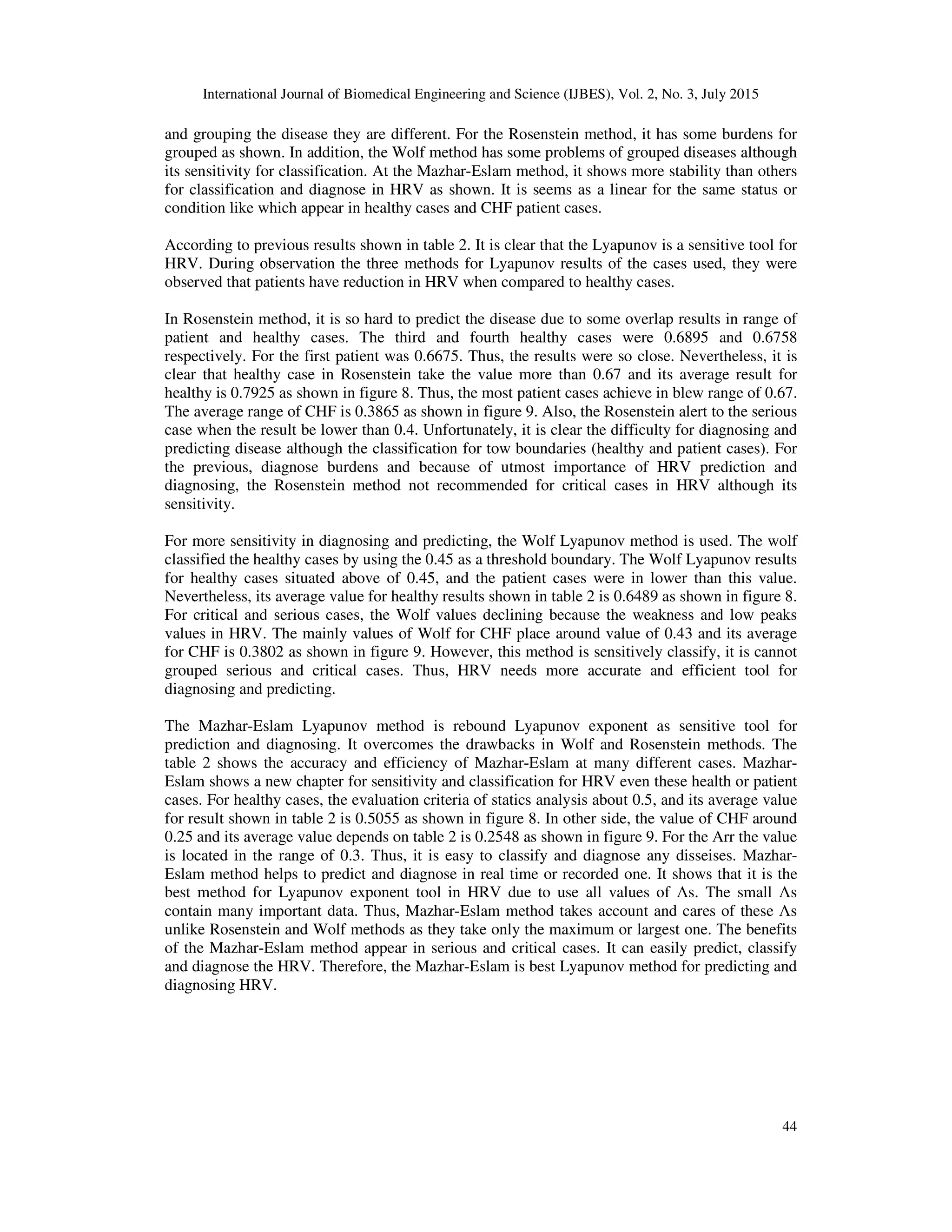
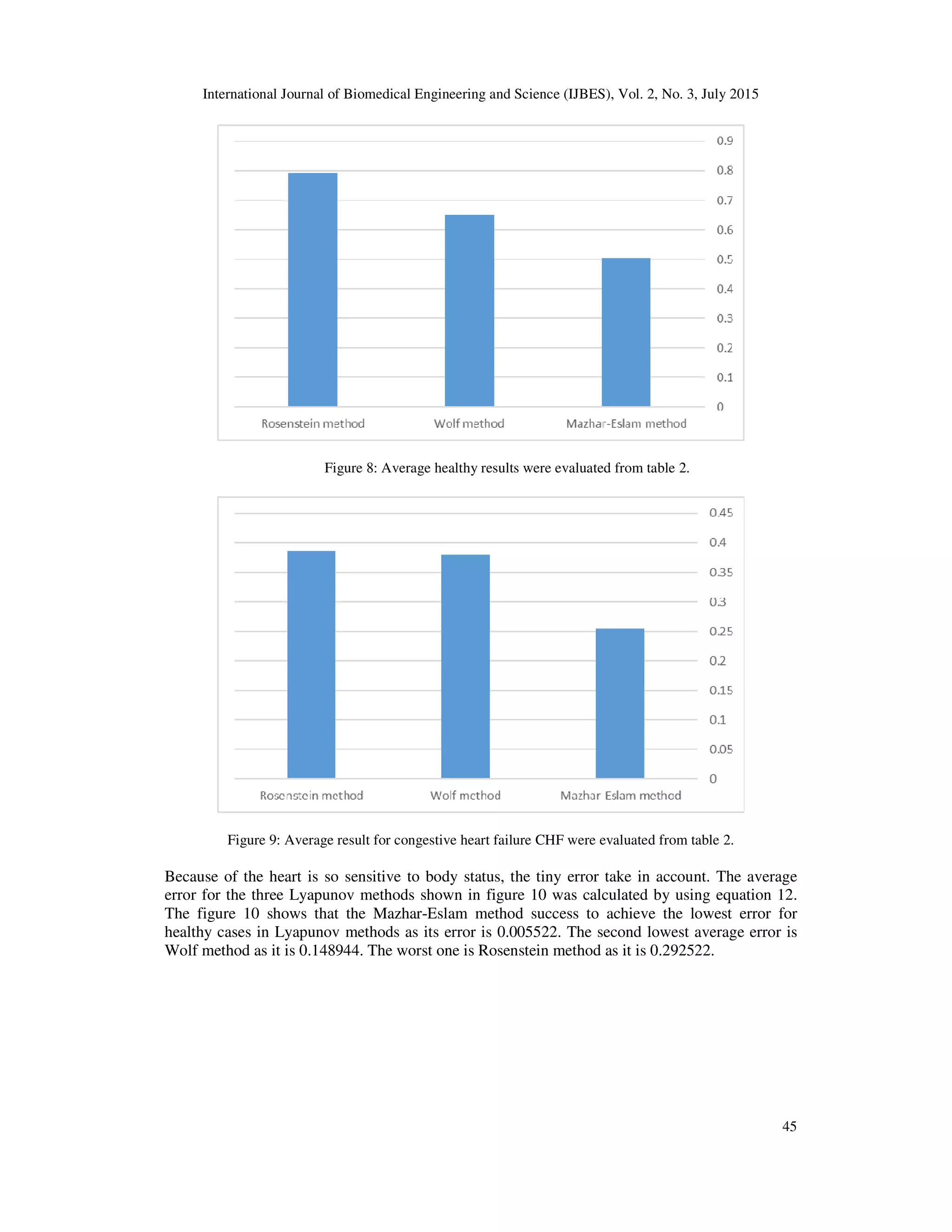
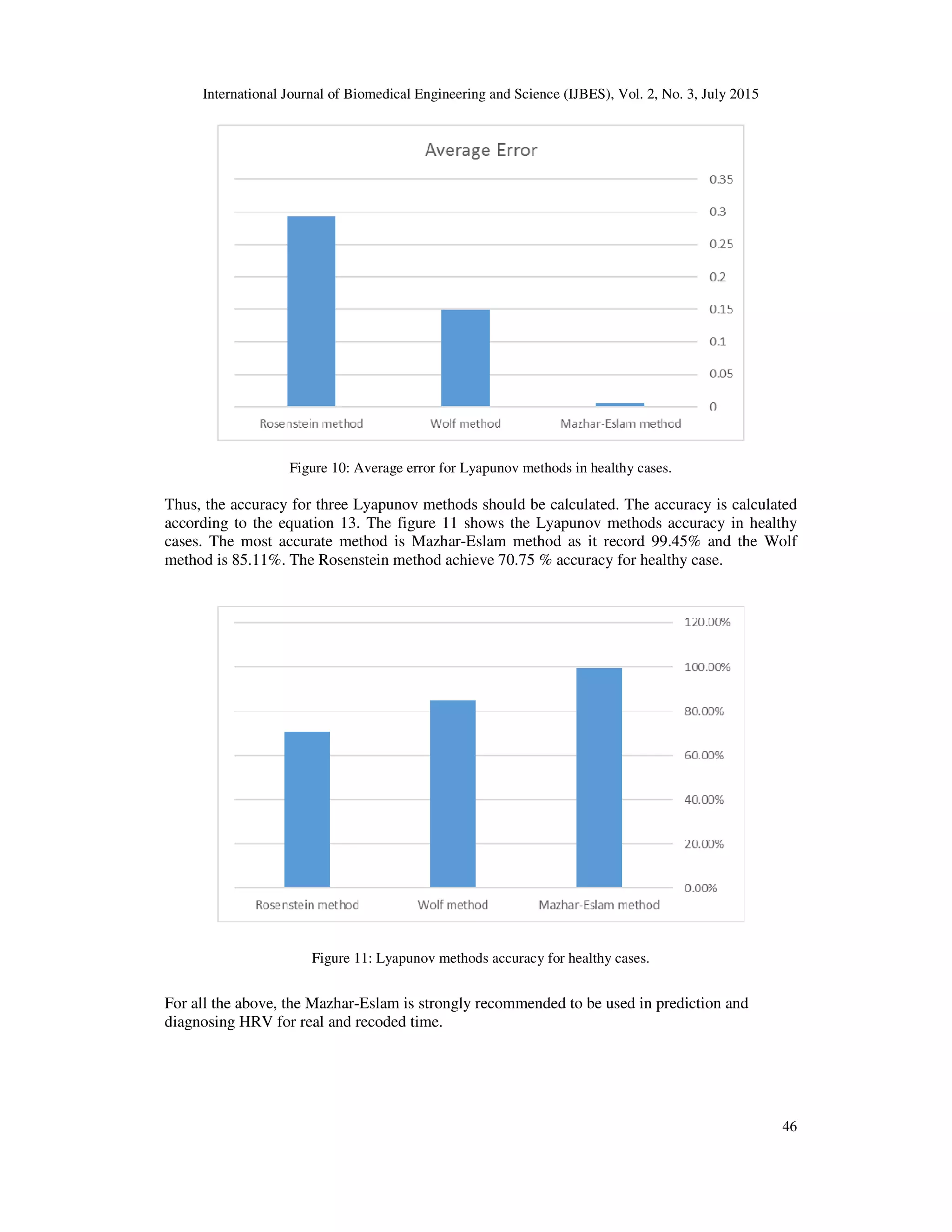
This paper presents a modified algorithm, Mazhar-Eslam, which enhances the Lyapunov exponent method to analyze heart rate variability (HRV) more accurately. HRV is essential for detecting cardiovascular risks and is influenced by both linear and nonlinear dynamics, highlighting the need for sensitive analysis tools. The study emphasizes the importance of HRV in understanding cardiac health and proposes an innovative approach for its analysis to aid in the prognostic evaluation of heart conditions.
![International Journal of Biomedical Engineering and Science (IJBES), Vol. 2, No. 3, July 2015
31
ROBUST AND SENSITIVE METHOD OF
LYAPUNOV EXPONENT FOR HEART RATE
VARIABILITY
Mazhar B. Tayel1
and Eslam I AlSaba2
1,2
Department of Electrical Engineering, Alexandria University, Alexandria, Egypt
ABSTRACT
Heart Rate Variability (HRV) plays an important role for reporting several cardiological and non-
cardiological diseases. Also, the HRV has a prognostic value and is therefore quite important in modelling
the cardiac risk. The nature of the HRV is chaotic, stochastic and it remains highly controversial. Because
the HRV has utmost importance, it needs a sensitive tool to analyze the variability. In previous work,
Rosenstein and Wolf had used the Lyapunov exponent as a quantitative measure for HRV detection
sensitivity. However, the two methods diverge in determining the HRV sensitivity. This paper introduces a
modification to both the Rosenstein and Wolf methods to overcome their drawbacks. The introduced
Mazhar-Eslam algorithm increases the sensitivity to HRV detection with better accuracy.
KEYWORDS
Heart Rate Variability, Chaotic system, Lyapunov exponent, Transform domain, and Largest Lyapunov
Exponent.
1. INTRODUCTION
Cardiovascular diseases are a growing problem in today’s society. The World Health
Organization (WHO) reported that these diseases make up about 30% of total global deaths.
Those heart diseases have no geographic, gender or socioeconomic boundaries [3]. Therefore,
early stage detection of cardiac irregularities and correct treatment are very important. This
requires a good physiological understanding of cardiovascular system.
Studying the fluctuations of heart beat intervals over time reveals a lot of information called heart
rate variability (HRV) analysis. A reduction of HRV has been reported in several cardiological
and non-cardiological diseases. In addition, HRV has a prognostic value and is therefore quite
significant in modelling the cardiac risk. HRV has already proved his usefulness and is based on
several articles that have reviewed the possibilities of HRV [1 - 5].
The fact that HRV is a result of both linear and nonlinear fluctuations opened new perspectives as
previous research was mostly restricted to linear techniques. Some situations or interventions can
change the linear content of the variability, while leaving the nonlinear fluctuations intact. In
addition, the reverse can happen: interventions, which up till now have been believed to leave
cardiovascular fluctuations intact based on observations with linear methods, can just as well
modify the nonlinear fluctuations. This can be important in the development of new drugs or
treatments for patients. This paper introduces a modification algorithm method to overcome the
drawbacks arising in both Rosenstein and Wolf methods using the same approach of Lyapunov
exponent. That analysis the nonlinear behaviour of the HRV signals. The modified method create
a new chapter of sensitivity of HRV by a new description for Lyapunov exponent. The modified
Mazhar-Eslam method achieve more accuracy than another Lyapunov methods Wolf and
Rosenstein.](https://image.slidesharecdn.com/robustandsensitivemethodof-150808042152-lva1-app6892/75/Robust-and-sensitive-method-of-1-2048.jpg)
![International Journal of Biomedical Engineering and Science (IJBES), Vol. 2, No. 3, July 2015
32
0 1000 2000 3000 4000 5000 6000 7000 8000 9000 10000
0
0.5
1
number of samples
bpm
2. HEART RATE VARIABILITY
Heart Rate Variability (HRV) is a phenomenon that describes temporal variation in intervals
between consecutive heartbeats in sinus rhythm. HRV refers to variations in beat-to-beat intervals
corresponding to instantaneous HRs. HRV is a reliable reflection of many physiological factors
modulating normal rhythm of heart. In fact, they provide a powerful means of observing interplay
between sympathetic and parasympathetic nervous systems. It shows that a structure generating a
signal is not only simply linear, but also involves nonlinear contributions.
Spontaneous variability of HR has been related to three major physiological originating factors:
quasi-oscillatory fluctuations thought to arise in blood-pressure control, variable frequency
oscillations due to thermal regulation, and respiration. Frequency selective analysis of cardiac
inter-beat interval sequences allows separate contributions to be isolated. Using this method, a
laboratory and field study of effects of mental work load on the cardiac interval sequence has
been carried out [4].
The diagnosticity of HR is restricted by several factors like environmental stressors and physical
demands that may be associated with a task. These tasks may have different physiological
consequences and change in HR may depends on these factors more than mental workload. Backs
(1998) [6] focused on the fact that observed HR could be caused by different underlying patterns
of autonomic nervous system activity. If different information processing demands affect the
heart via different modes of autonomic control, it could increase diagnosticity of HR [6]. Backs‟
study addressed the validity of the autonomic component, using data from a large study, in which
many central and peripheral psycho-8 physiological measures were collected simultaneously
while performing single and dual tasks which had different physical demands. The measures
collected were the residual HR, parasympathetic and sympathetic activity, respiratory sinus
arrhythmia (RSA), and THM (Traube-Hering-Mayer) wave using principle component analysis
(PCA), image factoring, impedance cardiogram (ZKG) and ElectroCardioGram (ECG). The
sympathetic and parasympathetic systems were examined for independence. From the study, the
PCA factors computed on raw ECG data provided useful information like different autonomic
modes of control were found that were not evident in heart period. The objective was to verify if
factors extracted using residual HR as a marker variable validly reflected cardiac sympathetic
activity and if the solutions obtained from raw and baseline corrected data were in compliance
with each other. This information about the underlying autonomic activity may increase the
diagnosticity of HR. Figure 1 shows the example of HR variation of normal subject (control
case).
Figure 1. Heart rate variation of normal subject.](https://image.slidesharecdn.com/robustandsensitivemethodof-150808042152-lva1-app6892/75/Robust-and-sensitive-method-of-2-2048.jpg)
![International Journal of Biomedical Engineering and Science (IJBES), Vol. 2, No. 3, July 2015
33
2.1 Components of Heart Rate
HRV was originally assessed by calculating the mean beat to beat heart rate commonly called the
RR interval, and its standard deviation measured on short term ECG. To date about 26 different
types of arithmetic manipulations of RR intervals have been used . Variable of interest for the
study was the RMSSD index. The RMSSD index is defined as the root mean square of the
differences of the successive RR intervals. MAX-MIN or peak-valley quantification of HRV is
the difference between the shortest RR interval during inspiration and longest during expiration.
RMSSD is a time domain measure of HRV. Recently spectral analysis of HRV has been
developed which transforms the signal from time domain to frequency domain. The power
spectrum of heart rate and blood pressure yields three major bands. A low frequency peak ranging
between .06 Hz to .15 Hz, a high frequency peak ranging between .15 Hz to .4 Hz and a very low
frequency peak below .05 Hz constitute the power spectrum [13]. The LF is associated with blood
pressure control, reflecting sympathetic activity. The HF is correlated with respiratory sinus
arrhythmia reflecting parasympathetic activity [13]. The VLF is linked with vasomotor control or
temperature control. The RR interval data obtained from ECG or other heart rate monitoring
devices can be analyzed using any mathematical tool like Fourier transformation or moving
average method [14]. Statistical significance can be tested using standard tests after the frequency
domain analysis. For the current study, in the first phase the raw data obtained from the heart rate
monitor was analyzed using both the time domain and the frequency domain measures. The data
further obtained from these analyses was tested for statistical significance using analysis of
variance (ANOVA).
2.2 Heart Rate Measures
Important information on the heart rate components can be summarized from the as the
components of HRV are markers of the sympathetic and parasympathetic activity. The low
frequency component is associated with blood pressure control or sympathetic activity. In
addition, it is high, when the person is in high strain conditions. The high frequency component is
an indicator of parasympathetic autonomic response. Also, it is an indicator of respiratory sinus
arrhythmia (RSA). Besides, it is reduced during heavy exertions and awkward postures. The ratio
of low to high frequency is an estimate of mental stress. It is used as an index of parasympathetic
and sympathetic balance. This ratio is correlated with high job strain, when high. The very low
frequency is linked with temperature control. It is Often seen as an unreliable measure.
Reduced HRV predicts sudden death and is a marker of fatal ventricular arrhythmia. This
reduction in HRV can be examined from time domain components like the RMSSD. All of these
components are responsible for the identification of increased cardiac reactivity in individuals
under high stress.
2.3 Practical Applications of Heart Rate Monitors
HRV is sensitive to both physiological and psychophysical disorders. In recent years HRV has
also been used as a tool to improve diagnosing of heart rate in the general population which
included both the working and non-working population. Assessing the impact of physical and
mental demands associated with tasks in a work place on the heart can help to predict cardiac
diseases. Therefore it has become essential to measure HRV [15].
Measurement of HRV in the past required a high-quality electrocardiogram (ECG), but the cost
and complexity of the ECG equipment has made it difficult to perform HRV analysis particularly](https://image.slidesharecdn.com/robustandsensitivemethodof-150808042152-lva1-app6892/75/Robust-and-sensitive-method-of-3-2048.jpg)
![International Journal of Biomedical Engineering and Science (IJBES), Vol. 2, No. 3, July 2015
34
in the physical training field [16]. To address these needs, several portable heart rate monitoring
devices have been designed. The development of wireless heart rate monitoring (HRM) with
elastic electrode belt allowing the detection of RR intervals with a resolution of 1ms represents an
interesting alternative to classic fixed or ambulatory ECG for use outside of laboratory settings.
Kingsley demonstrated that the R-R intervals and heart rate measurements obtained using Polar
810S and ambulatory ECG system are in good agreement with each other [16]. Gamelin
examined the validity of the Polar S810 monitor to measure RR intervals at rest. Narrow limits of
agreement, good correlation and small effect sizes validate the monitor and measure RR intervals
to make HRV analysis [15]. Sandercock measured the reliability of three commercially
available HRV instruments using short term recordings. These recordings were made in three
conditions: lying supine, standing, and lying supine with controlled breathing. Reliability was
calculated using CV (coefficient of variation), ICC (intraclass correlation coefficient) and LoA
(limits of agreement). The study showed supine condition is more reliable. On the whole the
short term recordings less than five minutes were seen to be unreliable [17].
On the whole heart rate monitors pave a simple pathway to measure the heart rate in a feasible
manner as they are affordable, portable, reliable for recordings more than 5 minutes and also easy
to handle. For this study the Polar RS800 monitor (Polar Electro Inc., Lake Success, NY) was
used to record the data. It has a chest strap and a watch which transmits data wirelessly. Previous
literature reviews showed that various heart rate monitors had been checked for their validity and
reliability. But the comfort levels experienced while using the heart rate monitor had not been
addressed. This is important because wearing a heart rate monitor in a real time situation during
work should not affect the workers performance and should be as comfortable as possible. One of
the purposes of this study was to see how comfortable the wearer feels while doing various tasks,
so that the HR monitor can be used for real time recording. Also statistical consistency had not
been tested thoroughly and there is little research on HRV during a physical or manual activity
like moving something heavy. Earlier studies had shown that the heart rate increases when a
manual material handling job is performed, but the spectral components had not been studied in
association with predictability of diseases [18].
3. LYAPUNOV EXPONENT
Lyapunov exponent Λ is a quantitative measure of the sensitive dependence on the initial
conditions. It defines the average rate of divergence or convergence of two neighbouring
trajectories in the state-space.Consider two points in a space, and , each of which will
generate an orbit in that space using system of equations as shown in figure 2.
Figure 2. Calculation for two neighbouring trajectories.](https://image.slidesharecdn.com/robustandsensitivemethodof-150808042152-lva1-app6892/75/Robust-and-sensitive-method-of-4-2048.jpg)
![International Journal of Biomedical Engineering and Science (IJBES), Vol. 2, No. 3, July 2015
35
These orbits are considered as parametric functions of a variable. If one of the orbits is used as a
reference orbit, then the separation between the two orbits will be a function of time. Because
sensitive dependence can arise only in some portions of a system, this separation is a location
function of the initial value and has the form . In a system with attracting fixed points or
attracting periodic points, decreases asymptotically with time. For chaotic points, the
function will behave unpredictably. Thus, it should study the mean exponential rate of
divergence of two initially closed orbits using the formula
(1)
This number, called the Lyapunov exponent "Λ". An exponential divergence of initially nearby
trajectories in state-space coupled with folding of trajectories, to ensure that the solutions will
remain finite, is the general mechanism for generating deterministic randomness and
unpredictability. Therefore, the existence of a positive Λ for almost all initial conditions in a
bounded dynamical system is the widely used definition of deterministic chaos. To discriminate
between chaotic dynamics and periodic signals, Λ s are often used. The trajectories of chaotic
signals in state-space follow typical patterns. Closely spaced trajectories converge and diverge
exponentially, relative to each other. A negative exponent the orbit attracts to a stable
fixed point or stable periodic orbit. Negative Lyapunov exponents are characteristic
of dissipative or non-conservative systems. Such systems exhibit asymptotic stability. The more
negative the exponent, the greater the stability. Super stable fixed points and super stable periodic
points have a Lyapunov exponent of Λ = − ∞. This is something similar to a critically damped
oscillator in that the system heads towards its equilibrium point as quickly as possible. A zero
exponent the orbit is a neutral fixed point (or an eventually fixed point). A Lyapunov
exponent of zero indicates that the system is in some sort of steady state mode. A physical system
with this exponent is conservative. Such systems exhibit Lyapunov stability. Take the case of two
identical simple harmonic oscillators with different amplitudes. Because the frequency is
independent of the amplitude, a phase portrait of the two oscillators would be a pair of concentric
circles. The orbits in this situation would maintain a constant separation. Finally, a positive
exponent implies the orbits are on a chaotic attractor. Nearby points, no matter how close, will
diverge to any arbitrary separation. These points are unstable [3]. The flowchart of the practical
algorithm for calculating largest Lyapunov exponents is shown in figure 3.
In the following, the Largest Lyapunov Exponent algorithms are discussed.](https://image.slidesharecdn.com/robustandsensitivemethodof-150808042152-lva1-app6892/75/Robust-and-sensitive-method-of-5-2048.jpg)
![International Journal of Biomedical Engineering and Science (IJBES), Vol. 2, No. 3, July 2015
36
Figure 3. Flowchart of the practical algorithm for calculating largest Lyapunov exponents
3.1. Wolf's Algorithm
Wolf’s algorithm [7] is straightforward and uses the formulas defining the system. It calculates
two trajectories in the system, each initially separated by a very small interval. The first trajectory
is taken as a reference, or ’fiducial’ trajectory, while the second is considered ’perturbed’. Both
are iterated together until their separation is large enough.
In this study, the two nearby points in a state-space and , that are function of time and
each of which will generate an orbit of its own in the state, the separation between the two orbits
∆x will also be a function of time. This separation is also a function of the location of the initial
value and has the form , where t is the value of time steps forward in the trajectory. For
chaotic data set, the mean exponential rate of divergence of two initially close orbits is
characterized by
(2)](https://image.slidesharecdn.com/robustandsensitivemethodof-150808042152-lva1-app6892/75/Robust-and-sensitive-method-of-6-2048.jpg)
![International Journal of Biomedical Engineering and Science (IJBES), Vol. 2, No. 3, July 2015
37
The maximum positive Λ is chosen as .
Largest Lyapunov exponent’s quantify sensitivity of the system to initial conditions and gives a
measure of predictability. This value decreases for slowly varying signals like congenital heart
block (CHB) and Ischemic/dilated cardiomyopathyand will be higher for the other cases as the
variation of RR is more [8, 9]. The LLE is 0.505 for the HR signalshown in Figure 1.
3.2. Rosenstein's Algorithm
Rosenstein’s algorithm [10] works on recorded time-series, where the system formulas may not
be available. It begins by reconstructing an approximation of the system dynamics by embedding
the time-series in a phase space where each point is a vector of the previous m points in time (its
’embedding dimension’), each separated by a lag of j time units. Although Taken’s theorem [11]
states that an embedding dimension of 2D + 1 is required to guarantee to capture all the dynamics
of a system of order D, it is often sufficient in practice to use m = D. Similarly, although an
effective time lag must be determined experimentally, in most cases j = 1 will suffice.
Given this embedding of the time-series, for each point founding its nearest neighbour (in the
Euclidean sense) whose temporal distance is greater than the mean period of the system,
corresponding to the next approximate cycle in the system’s attractor. This constraint positions
the neighbours as a pair of slightly separated initial conditions for different trajectories. The mean
period was calculated as the reciprocal of the mean frequency of the power spectrum of the time-
series calculated in the usual manner using the Fast Fourier Transform (FFT). As shown in figure
3.
Now it can be performed a process similar to Wolf’s algorithm to approximate the Largest
Lyapunov Exponent (LLE). The first step of this approach involves reconstructing the attractor
dynamics from the RR interval time series. After reconstructing the dynamics, the algorithm
locates the nearest neighbour of each point on the trajectory. The nearest neighbour, , is found
by searching for the point that minimizes the distance to the particular reference point, . This is
expressed as:
(3)
where is the initial distance from the point to its nearest neighbour and || ... || denotes the
Euclidean norm. An additional constraint is imposed, namely that nearest neighbours have a
temporal separation greater than the mean period of the RR interval time series. Therefore, one
can consider each pair of neighbours as nearby initial conditions for different trajectories. The
largest Lyapunov exponent (LLE) is then estimated as the mean rate of separation of the nearest
neighbours. More concrete, it is assumed that the pair of nearest neighbours diverge
approximately at a rate given by the largest Lyapunov exponent :
(4)
By taking the ln of both sides of this equation:
(5)
which represents a set of approximately parallel lines (for j = 1, 2, . . . ,M), each with a slope
roughly proportional to .](https://image.slidesharecdn.com/robustandsensitivemethodof-150808042152-lva1-app6892/75/Robust-and-sensitive-method-of-7-2048.jpg)
![International Journal of Biomedical Engineering and Science (IJBES), Vol. 2, No. 3, July 2015
38
The natural logarithm of the divergence of the nearest neighbour to the jth
point in the phase space
is presented as a function of time. The largest Lyapunov exponent is then calculated as the slope
of the ’average’ line, defined via a least squares fit to the ’average’ line defined by:
(6)
where denotes the average over all values of j. This process of averaging is the key to
calculating accurate values of using smaller and noisy data sets compared to other Lyapunov
algorithms. The largest Lyapunov exponent (LLE) is 0.7586 for the HR signalshown in Figure 1.
3.3.The calculations
The exponents were calculated using the Wolf and Rosenstein algorithms implemented as
previously recommended. For both algorithms, the first two steps were similar. An embedded
point in the attractor was randomly selected, which was a delay vector with dE elements
(7)
This vector generates the reference trajectory. It's nearest neighbour vector
(8)
was then selected on another trajectory by searching for the point that minimizes the distance to
the particular reference point. For the Rosenstein algorithm, it is imposed the additional constraint
that the nearest neighbour has a temporal separation greater than the mean period of the time
series defined as the reciprocal of the mean frequency of the power spectrum.
The two procedures then differed. For the Wolf algorithm, the divergence between the two
vectors was computed and as the evolution time was higher than three sample intervals, a new
neighbour vector was considered. This replacement restricted the use of trajectories that shrunk
through a folding region of the attractor. The new vector was selected to minimize the length and
angular separation with the evolved vector on the reference trajectory. This procedure was
repeated until the reference trajectory has gone over the entire data sample and k1 was estimated
as:
(9)
where and are the distance between the vectors at the beginning and end of a
replacement step, respectively, and M is the total number of replacement steps. Note this equation
uses the natural logarithm function and not the binary logarithm function as presented by Wolf
[7]. This change makes Λm exponents more comparable between the two algorithms.
For the Rosenstein algorithm, the divergence d (t) between the two vectors was computed at each
time step over the data sample. Considering that embedded points (delay vectors)
composed the attractor, the above procedure was repeated for all of them and Λm were then
estimated from the slope of linear fit to the curve defined by:
(10)](https://image.slidesharecdn.com/robustandsensitivemethodof-150808042152-lva1-app6892/75/Robust-and-sensitive-method-of-8-2048.jpg)
![International Journal of Biomedical Engineering and Science (IJBES), Vol. 2, No. 3, July 2015
39
where represents the mean logarithmic divergence for all pairs of nearest neighbours
over time. . This process of averaging is the key to calculating accurate values of using smaller
and noisy data sets compared to Wolf algorithms.
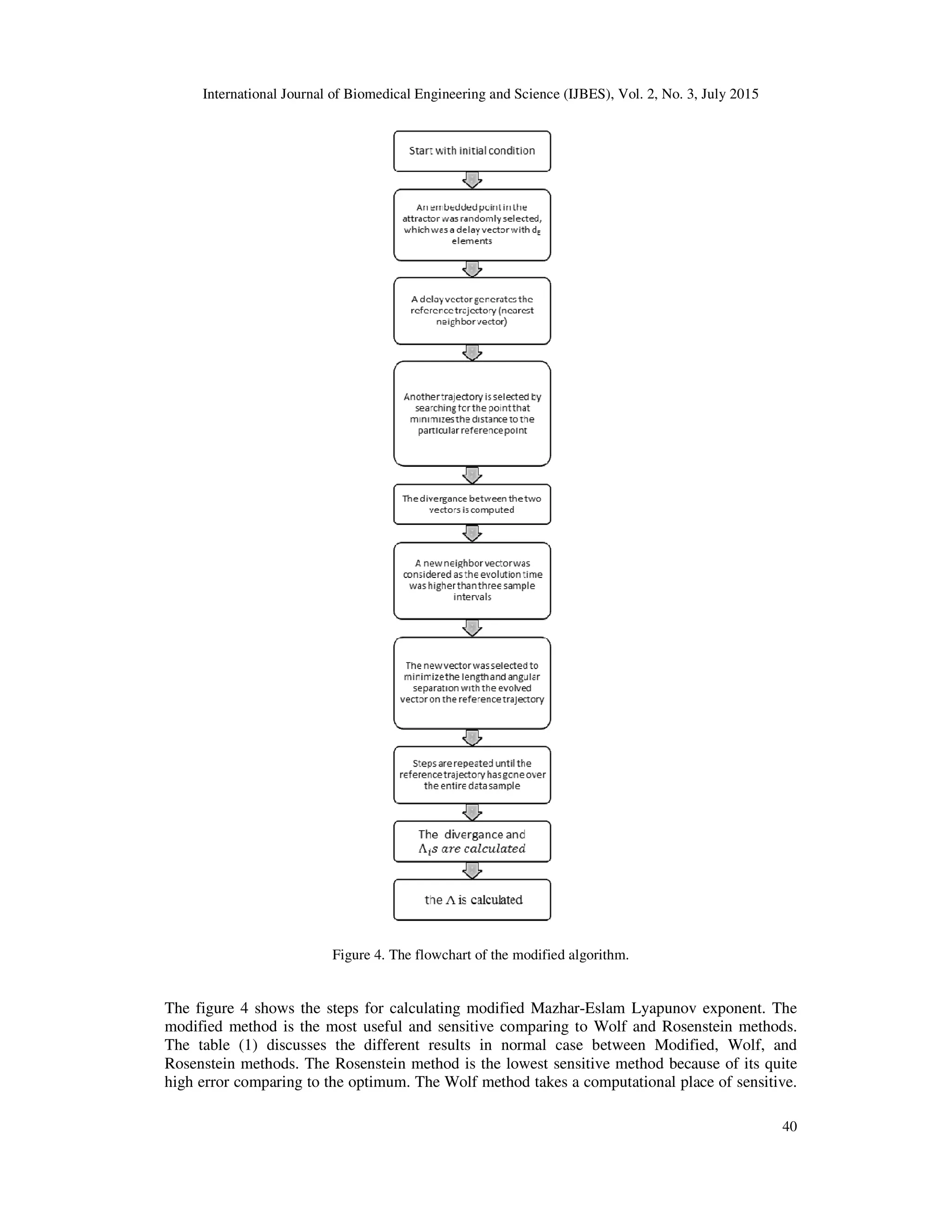
3.4.The modified Mazhar-Eslam Lyapunov Exponent
The modified algorithm steps are same Rosenstein's algorithm steps. However, the Rosenstein's
algorithm uses the Fast Fourier Transform (FFT) as shown in figure 3; the modified algorithm
uses the Discrete Wavelet Transform (DWT) as shown in figure 4. That it is because DWT
advantages comparing with FFT. In the next some reasons to choose DWT instead of FFT.
3.4.1. Preference for choosing DWT instead of FFT
Although the FFT has been studied extensively, there are still some desired properties that are not
provided by FFT. This section discusses some points are lead to choose DWT instead of FFT.
The first point is hardness of FFT algorithm pruning. When the number of input points or output
points are small comparing to the length of the DWT, a special technique called pruning is often
used [12]. However, it is often required that those non-zero input data are grouped together. FFT
pruning algorithms does not work well when the few non-zero inputs are randomly located. In
other words, sparse signal does not give rise to faster algorithm.
The other disadvantages of FFT are its speed and accuracy. All parts of FFT structure are one
unit and they are in an equal importance. Thus, it is hard to decide which part of the FFT structure
to omit when error occurring and the speed is crucial. In other words, the FFT is a single speed
and single accuracy algorithm.
The other reason for not selecting FFT is that there is no built-in noise reduction capacity.
Therefore, it is not useful to be used. According to the previous ,the DWT is better than FFT
especially in Lyapunov exponent calculations when be used in HRV, because each small variant
in HRV indicates the important data and information. Thus, all variants in HRV should be
calculated.
3.4.2. Modified calculation of Largest Lyapunov Exponent Λ
The modified method depends on Rosenstein algorithm’s strategy with replacing the FFT by
DWT to estimate lag and mean period. However, the modified method use the same technique of
Wolf technique for Λm calculating except the first two steps and the final step as they are taken
from Rosenstein’s method. The Lyapunov exponent (Λ) measures the degree of separation
between infinitesimally close trajectories in phase space. As discussed before, the Lyapunov
exponent allows determining additional invariants. The modified method of LLE (Λ) is calculated
as
(11)
Note that the s contain the maximum Λ and variants Λs that indicate to the helpful and
important data. Therefore, the modified Lyapunov is a more sensitive prediction tool. Thus, it is
robust predictor for real time, in addition to its sensitivity for all time whatever the period. It is
found that the modified largest Lyapunov exponent (Λm) is 0.4986 for the HR signal shown in
Figure 1. Thus, it is more accurate than Wolf and Rosenstein Lyapunov exponent.](https://image.slidesharecdn.com/robustandsensitivemethodof-150808042152-lva1-app6892/75/Robust-and-sensitive-method-of-9-2048.jpg)
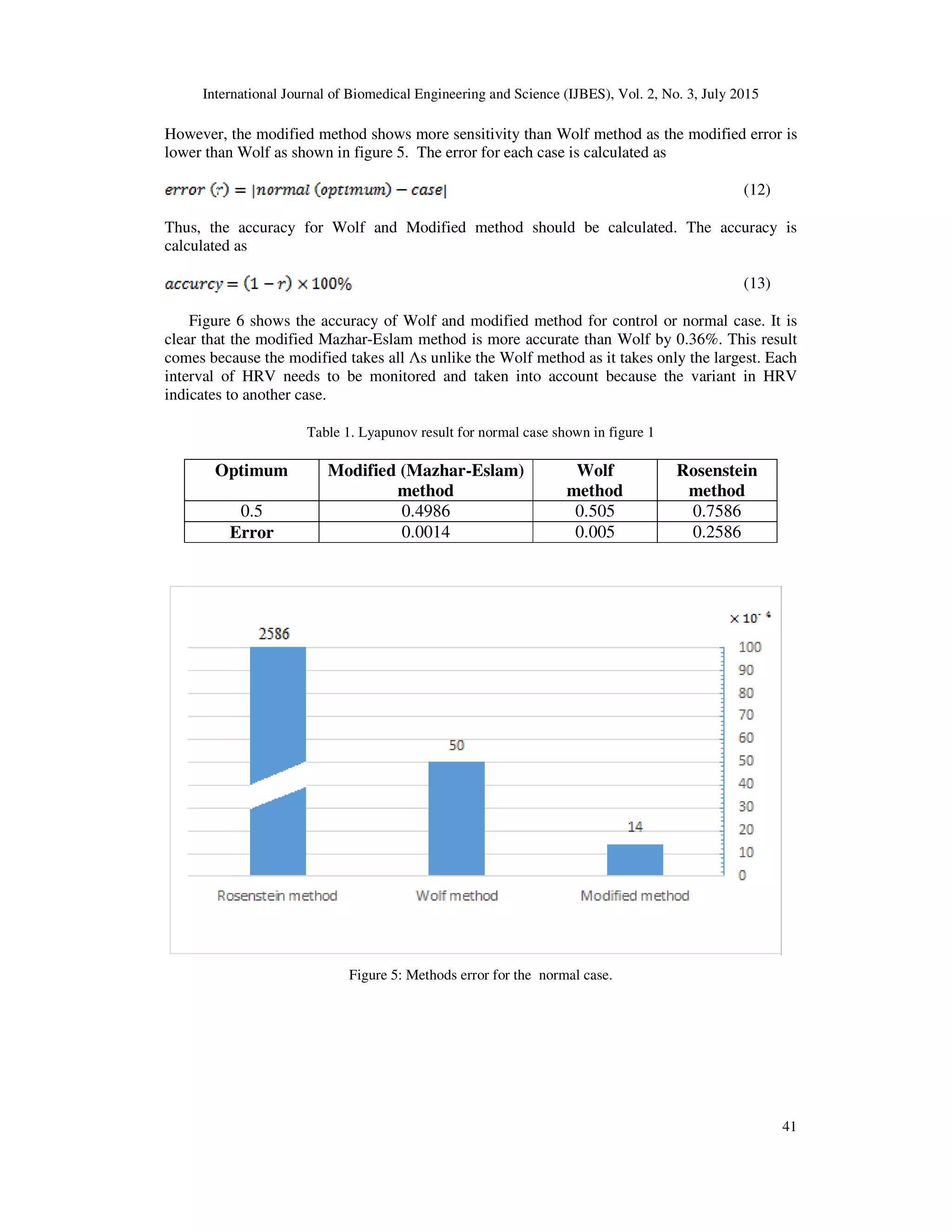
![International Journal of Biomedical Engineering and Science (IJBES), Vol. 2, No. 3, July 2015
47
5. CONCLUSIONS
Heart Rate Variability (HRV) is reported in several cardiological and non-cardiological diseases.
Also, it has a prognostic value and is therefore very important in modelling the cardiac risk. HRV
is chaotic or stochastic remains highly controversial. In order to have utmost importance, HRV
needs a sensitive tool to analyze it like Lyapunov exponent as it is a quantitative measure of
sensitivity. While the Λm from both Lyapunov exponent algorithms were nearly equal for small
heart rate (HR) data sets. The Rosenstein algorithm provided less sensitive Λm estimates than the
Wolf algorithm to capture differences in local dynamic stability from small gait data sets. The
data supported the idea that this latter outcome results from the ability and inability of the Wolf
algorithm and Rosenstein algorithm, respectively, to estimate adequately Λm of attractors with an
important rate of convergence as those in gait. Indeed, it was found that the Wolf algorithm
makes an excellent use of the attractor divergences for estimating Λm while the Rosenstein
algorithm overlooks the attractor expansion. Therefore, the Wolf algorithm appears to be more
appropriate than the Rosenstein algorithm to evaluate local dynamic stability from small gait data
sets like HRV. Increase in the size of data set has been shown to make the results of the
Rosenstein algorithm more suitable, although other means as increasing the sample size might
have a similar effect. The modified Mazhar-Esalm method combines Wolf and Rosenstein
method. It takes the same strategy of Rosenstein method for initial step to calculate the lag and
mean period, but it uses Discrete Wavelet Transform (DWT) instead of Fats Fourier Transform
(FFT) unlike Rosenstein. After that, it completes steps of calculating Λs as Wolf method. The
modified Mazhar-Eslam method care of all variants especially the small ones like that are in
HRV. These variants may contain many important data to diagnose diseases as RR interval has
many variants. Thus, the modified Mazhar-Eslam method of Lyapunov exponent Λ takes all of
Λs. That leads it to be robust predictor and that appear in different results between modified
Mazhar-Eslam, Wolf, and Rosenstein. The Mazhar-Eslam is more accurate than Wolf and
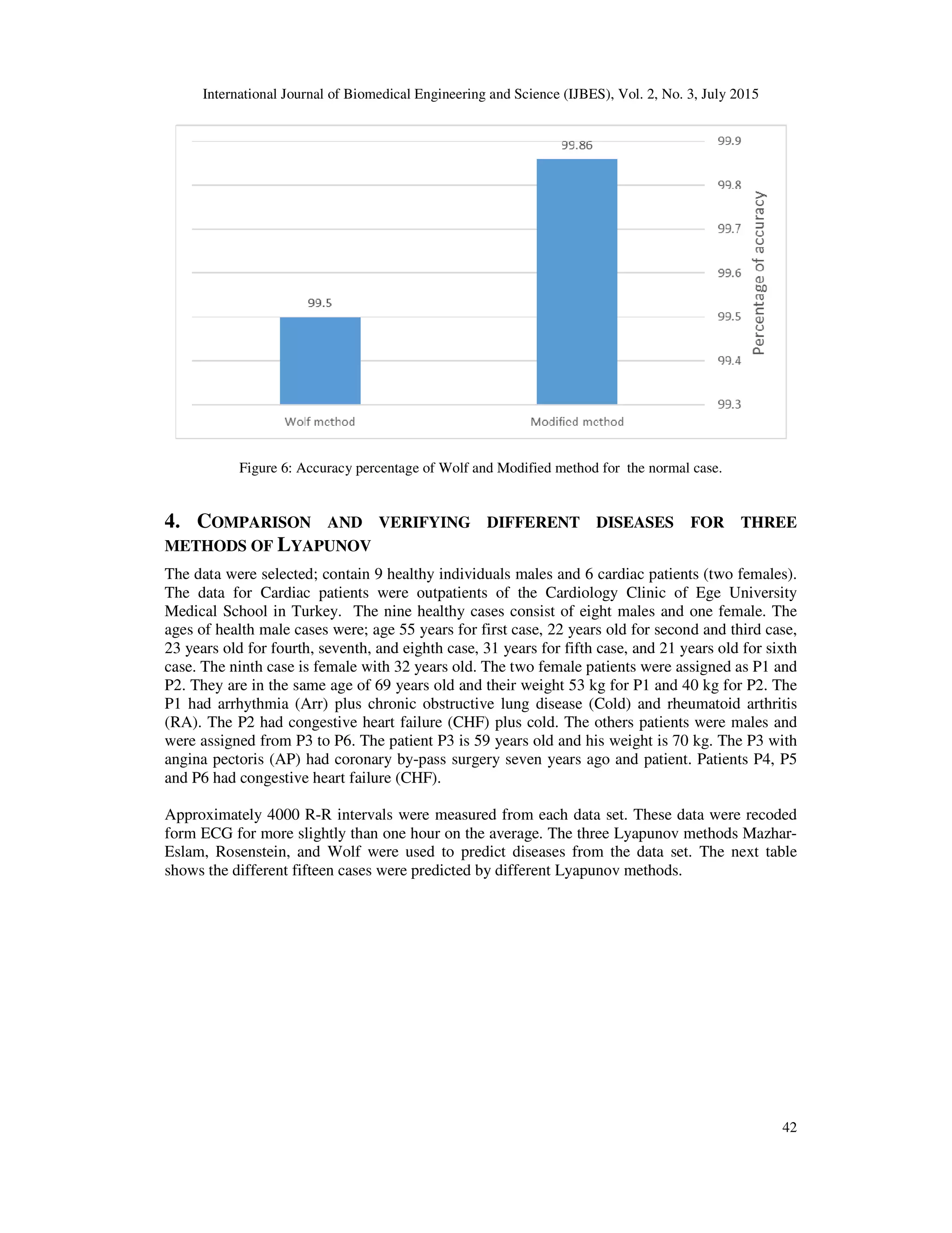
Rosenstein Lyapunov exponent. The accuracy of modified Mazhar-Eslam method for control or
normal case is more accurate than Wolf by 0.36%. However, for healthy cases, the Mazhar-Eslam
is more accurate than wolf by 14.34%.
REFERENCES
[1] A.E. Aubert and D. Ramaekers. Neurocardiology: the benefits of irregularity. The basics of
methodology, physiology and current clinical applications. ActaCardiologica, 54(3):107–120, 1999.
[2] Task Force of the European Society of Cardiology and the North American Society of Pacing and
Electrophysiology. Heart rate variability: standards of measurement, physiological interpretation and
clinical use. Circulation, 93:1043–1065, 1996.
[3] U. RajendraAchrya, K. Paul Joseph, N. Kannathal, Choo Min Lim, Jasjit S. Suri. "Heart Rate
Variability: a review" Med Bio EngComput (2006) 44:1031-1051
[4] P.K. Stein and R.E. Kleiger. Insights from the study of heart rate variability. Annual Review of
Medicine, 50(1):249–261, 1999.
[5] Y. Gang and M. Malik. Heart rate variability analysis in general medicine. Indian Pacing and
Electrophysiology Journal, 3(1):34–40, 2003.
[6] Backs, R. W. (1998). A comparison of factor analytic methods of obtaining cardiovascular autonomic
components for the assessment of mental work load. [heart rate analysis]. Ergonomics. 41, 733-745.
[7] WOLF, A., SWIFT, J., SWINNEY, H., AND VASTANO, J. Determining lyapunov exponents from a
time series Physica D: Nonlinear Phenomena 16, 3 (July 1985), 285–317.
[8] Acharya UR, Kannathal N, Krishnan SM (2004) Comprehensive analysis of cardiac health using heart
rate signals.
[9] Acharya UR, Kannathal N, Seng OW, Ping LY, Chua T (2004) Heart rate analysis in normal subjects
of various age groups. Biomed Online J USA 3(24)
[10] ROSENSTEIN, M. T., COLLINS, J. J., AND DE LUCA, C. J. A practical method for calculating
largest lyapunov exponents from small data sets. Phys. D 65, 1-2 (1993), 117–134.
[11] Takens F 1981 Detecting strange attractors in turbulence Springer Lecture Notes in Mathematics vol
898, pp 366–81](https://image.slidesharecdn.com/robustandsensitivemethodof-150808042152-lva1-app6892/75/Robust-and-sensitive-method-of-17-2048.jpg)
![International Journal of Biomedical Engineering and Science (IJBES), Vol. 2, No. 3, July 2015
48
[12] H.V. Sorensen and C.S. Burrus.Efficient computation of the DFT with only a subset of input or output
points. IEEE Transactions on Signal Processing, 41(3): 1184-1200, March 1993.
[13] Kamath, M. V., and Fallen, E.L. (1993). Power spectral analysis of heart rate variability: A non
invasive signature of cardiac autonomic function. Critical Reviews in Biomedical Engineering, 21(3),
345-311.
[14] Quintana, M., Storckt, N., Lindbald, L.E., Lindvall, K., and Ericson, M. (1997). Heart rate variability
as a means of assessing prognosis after acute myocardial infarction. European Heart Journal,18(5),
789-797.
[15] Gamelin, X. F., Berthoin, S., and Bosquet, L. (2006). Validity of the Polar S810 Heart Rate Monitor
to Measure R–R Intervals at Rest. Medicine and Science in Sports and Exercise 38(5), 887-893.
[16] Kingsley, M., Lewis, M. J., and Marson R. E. (2005). Comparison of Polar 810S and an ambulatory
ECG system for RR interval measurement during progressive exercise. International Journal of Sports
Medicine, 26, 39-44.
[17] Sandercock, G. R. H., Bromley, P., and Brodie, D.A. (2004). Reliability of three commercially
available heart rate variability instruments using short term (5 min) recordings. Clinical Physiological
Function Imaging, 24(6), 359-367.
[18] Garg, A., and Saxena, U. (1979). Effects of lifting frequency and technique on physical fatigue with
special reference to psychophysical methodology and metabolic rate. American Industrial Hygiene
Association Journal, 40(10), 894-903.
AUTHORS
Mazhar B. Tayel was born in Alexandria, Egypt on Nov. 20th, 1939. He was graduated
from Alexandria University Faculty of Engineering Electrical and Electronics department
class 1963. He published many papers and books in electronics, biomedical, and
measurements.Prof. Dr. Mazhar Bassiouni Tayel had his B.Sc. with honor degree in 1963,
and then he had his Ph.D. Electro-physics degree in 1970. He had this Prof. degree of
elect. and communication and Biomedical Engineering and systems in 1980. Now he is
Emeritus Professor since 1999. From 1987 to 1991 he worked as a chairman,
communication engineering section, EED BAU-Lebanon and from 1991 to 1995 he worked as Chairman,
Communication Engineering Section, EED Alexandria. University, Alexandria Egypt, and from 1995 to
1996 he worked as a chairman, EED, Faculty of Engineering, BAU-Lebanon, and from 1996 to 1997 he
worked as the dean, Faculty of Engineering, BAU - Lebanon, and from 1999 to 2009 he worked as a senior
prof., Faculty of Engineering, Alexandria. University, Alexandria Egypt, finally from 2009 to now he
worked as Emeritus Professor, Faculty of Engineering, Alexandria University, Alexandria Egypt. Prof. Dr.
Tayel worked as a general consultant in many companies and factories also he is Member in supreme
consul of Egypt. E.Prof. Mazhar Basyouni Tayel
Eslam Ibrahim ElShorbagy AlSaba was born in Alexandria, Egypt on July. 18th, 1984.
He was graduated from Arab Academy for Science Technology and Maritime Transport
Faculty of Engineering and Technology Electronics and Communications Engineering
department class 2007. He published many papers in signal processing.Eslam Ibrahim
AlSaba had his B.Sc. with honor degree in 2007, and then he had his MSc. Electronics and
Communications Engineering degree in 2010. He is a PhD. Student in Alexandria
university Faculty of Engineering Electrical department Electronics and Communications Engineering
section from 2011 until now. From 2011 until now, he works as a researcher in Alexandria University. In
addition, now he works as a lecturer in Al Baha International college of Science, KSA.](https://image.slidesharecdn.com/robustandsensitivemethodof-150808042152-lva1-app6892/75/Robust-and-sensitive-method-of-18-2048.jpg)


![Guidelines heart rate_variability_ft_1996[1]](https://cdn.slidesharecdn.com/ss_thumbnails/guidelinesheartratevariabilityft19961-100604162052-phpapp01-thumbnail.jpg?width=640&height=640&fit=bounds)


