This document summarizes a numerical trajectory optimization method for path planning of multiple autonomous ground vehicles to avoid obstacles. It discretizes the continuous optimization problem into a nonlinear programming problem by approximating states with piecewise cubic polynomials and control with piecewise linear functions. The cost function accounts for minimizing time, distance to goal, and control effort. Constraints ensure obstacle and inter-vehicle distance avoidance. Simulation results show the effect of increasing node points in improving trajectory tracking accuracy.
Some experiments done on MATLAB for the course on Simulation and Modelling. Includes Model of Bouncing Ball, Model of Spring Mass System and Model of Traffic Flow.
Probabilistic Matrix Factorization (PMF)
Bayesian Probabilistic Matrix Factorization (BPMF) using
Markov Chain Monte Carlo (MCMC)
BPMF using MCMC – Overall Model
BPMF using MCMC – Gibbs Sampling
D I G I T A L C O N T R O L S Y S T E M S J N T U M O D E L P A P E R{Wwwguest3f9c6b
This document contains questions from a digital control systems exam. It covers topics like digital to analog conversion, z-transforms, stability analysis of sampled data systems, time domain analysis of discrete time systems using block diagrams, root locus analysis in the z-domain, controller design techniques like lead compensation, state space modeling, and stability analysis using Lyapunov's theorem. The exam has 8 questions with multiple parts that can be answered in the allotted time of 3 hours.
no U-turn sampler, a discussion of Hoffman & Gelman NUTS algorithmChristian Robert
The document describes the No-U-Turn Sampler (NUTS), an extension of Hamiltonian Monte Carlo (HMC) that aims to avoid the random walk behavior and poor mixing that can occur when the trajectory length L is not set appropriately. NUTS augments the model with a slice variable and uses a deterministic procedure to select a set of candidate states C based on the instantaneous distance gain, avoiding the need to manually tune L. It builds up a set of possible states B by doubling a binary tree and checking the distance criterion on subtrees, then samples from the uniform distribution over C to generate proposals. This allows NUTS to automatically determine an appropriate trajectory length and avoid issues like periodicity that can plague
This document proposes a method for continuous time series alignment in human action recognition. It defines continuous versions of time series, warping paths, and the dynamic time warping (DTW) distance. The method finds the optimal continuous warping path by approximating solutions to a cost minimization problem. An experiment applies the continuous DTW to classify human activities from accelerometer data, achieving classification accuracy close to the discrete DTW method. The continuous approach solves issues with resampling data and has potential for improved approximations and optimization methods.
The slide covers a few state of the art models of word embedding and deep explanation on algorithms for approximation of softmax function in language models.
1) The document presents the Low-Rank Regularized Heterogeneous Tensor Decomposition (LRRHTD) method for subspace clustering. LRRHTD seeks orthogonal projection matrices for all but the last tensor mode, and a low-rank projection matrix imposed with nuclear norm for the last mode, to obtain the lowest rank representation that reveals global sample structure for clustering.
2) LRRHTD models an Mth-order tensor dataset as a (M+1)th-order tensor by concatenating individual samples. It aims to find M orthogonal factor matrices for intrinsic representation and the lowest rank representation using the mapped low-dimensional tensor as a dictionary.
3) LRRHTD formulates an
This poster was created in LaTeX on a Dell Inspiron laptop with a Linux Fedora Core 4 operating system. The background image and the animation snapshots are dxf meshes of elastic waveform solutions, rendered on a Windows machine using 3D Studio Max.
The document discusses transportation problems and assignment problems in operations research. It provides:
1) An overview of transportation problems, including the mathematical formulation to minimize transportation costs while meeting supply and demand constraints.
2) Methods for obtaining initial basic feasible solutions to transportation problems, such as the North-West Corner Rule and Vogel's Approximation Method.
3) Techniques for moving towards an optimal solution, including determining net evaluations and selecting entering variables.
4) The formulation and algorithm for solving assignment problems to minimize assignment costs while ensuring each job is assigned to exactly one machine.
The document discusses approximation algorithms and genetic algorithms for solving optimization problems like the traveling salesman problem (TSP) and vertex cover problem. It provides examples of approximation algorithms for these NP-hard problems, including algorithms that find near-optimal solutions within polynomial time. Genetic algorithms are also presented as an approach to solve TSP and other problems by encoding potential solutions and applying genetic operators like crossover and mutation.
The document provides an overview of convex optimization problems, including linear programming (LP), quadratic programming (QP), quadratic constraint quadratic programming (QCQP), second-order cone programming (SOCP), and geometric programming. It discusses how these problems can be transformed into equivalent convex optimization problems to help solve them. Local optima are guaranteed to be global optima for convex problems. Optimality criteria are presented for problems with differentiable objectives.
Three sentences:
The document summarizes techniques for meshing and re-meshing used in computer graphics. It discusses using Voronoi diagrams and Delaunay triangulations to reconstruct meshes from point clouds, and using centroidal Voronoi tessellations to improve existing meshes through re-meshing by minimizing quantization noise. The document outlines methods for reconstruction, re-meshing scanned meshes, and converting meshes to subdivision surfaces.
Optimal Transport for a Computer Programmer's Point of ViewBruno Levy
This document summarizes optimal transport and provides an elementary introduction. It describes the optimal transport problem of finding a transport map that moves mass from one distribution to another while minimizing costs. This is relaxed using the Kantorovich formulation, which finds a transport plan rather than a map. Duality is also introduced, showing the equivalence between the primal problem of minimizing costs and the dual problem of maximizing a function. The relationship is explained using a discrete version of the transport problem.
This document discusses linear time-invariant (LTI) systems and convolution. Convolution is a fundamental concept in signal processing that is used to determine the output of an LTI system given its impulse response and an input signal. The convolution of two signals is obtained by decomposing the input signal into scaled and shifted impulses, taking the scaled and shifted impulse response for each impulse, and summing them to find the overall output. Convolution amplifies or attenuates different frequency components of the input independently. It plays an important role in applications like image processing and edge detection. Examples are provided to demonstrate evaluating convolution of periodic sequences.
Task Constrained Motion Planning for Snake RobotGiovanni Murru
Presentation of the work I've done during the Mobile Robotics course, about the task constrained motion planning for a snake-like robot with 24 dof, using probabilistic planning RRT to handle the task.
The document describes the octagon abstract domain, which is used in abstract interpretation of programs. It can represent relationships between two variables, such as X - Y ≤ c, using difference bound matrices. The octagon domain is more precise than the interval domain as it is relational, but has lower complexity than the polyhedra domain. Abstract transfer functions corresponding to semantic operations are used to manipulate elements in the domain. Shortest path closure is used to obtain the smallest representation. An example analysis and conclusion are also outlined.
This document describes a software tool called Polynomial Lattice Builder that is used to construct rank-1 polynomial lattice rules for quasi-Monte Carlo integration. It discusses the motivation for the tool, theoretical background on rank-1 polynomial lattice rules and figures of merit, an overview of the tool's features, examples of its applications, and conclusions. The tool allows users to choose parameters like the number of points, polynomial, dimension and construction method to generate optimal rank-1 polynomial lattice rules for their application.
This document presents an outer approximation solution algorithm for solving reliable shortest path problems on transportation networks. The algorithm formulates the problem as a mixed integer conic quadratic program to minimize the mean plus standard deviation of path costs. It then uses an outer approximation approach to decompose the problem and solve it efficiently through alternating steps of solving a master problem and subproblem. Computational results on several test networks show the algorithm converges quickly and outperforms directly solving the large-scale mixed integer conic quadratic program. The approach can also be applied to other reliability metrics and joint inventory location problems.
This document describes a Matlab project assignment on signal processing and the discrete Fourier transform (DFT). The project has two parts:
1) Developing functions for circular convolution properties like flipping, shifting, and convolution. Testing these functions with example signals.
2) Implementing block convolution using overlap-add and overlap-save strategies. Writing Matlab functions to perform overlap-add and overlap-save block convolution, and testing them with example data. Guidelines are provided for writing the project report.
This document summarizes a course on numerical optimal transport given by Bruno Lévy. It discusses the goals and motivations behind optimal transport, providing an elementary introduction. Specifically, it covers:
1) Monge's formulation of optimal transport as finding a map that transports one distribution into another while minimizing movement.
2) Kantorovich's relaxation of this to finding a transport plan between distributions rather than a map.
3) The use of duality to solve the optimal transport problem via a minimization-maximization approach rather than directly solving the Monge or Kantorovich problems.
Spline interpolation is a problem of "Numerical Methods".
This slide covers the basics of spline interpolation mostly the linear spline and cubic spline interpolation.
Digital Signal Processing[ECEG-3171]-Ch1_L03Rediet Moges
This Digital Signal Processing Lecture material is the property of the author (Rediet M.) . It is not for publication,nor is it to be sold or reproduced.
#Africa#Ethiopia
Why should you care about Markov Chain Monte Carlo methods?
→ They are in the list of "Top 10 Algorithms of 20th Century"
→ They allow you to make inference with Bayesian Networks
→ They are used everywhere in Machine Learning and Statistics
Markov Chain Monte Carlo methods are a class of algorithms used to sample from complicated distributions. Typically, this is the case of posterior distributions in Bayesian Networks (Belief Networks).
These slides cover the following topics.
→ Motivation and Practical Examples (Bayesian Networks)
→ Basic Principles of MCMC
→ Gibbs Sampling
→ Metropolis–Hastings
→ Hamiltonian Monte Carlo
→ Reversible-Jump Markov Chain Monte Carlo
Fourier-transform analysis of a unilateral fin line and its derivativesYong Heui Cho
This document presents a Fourier-transform analysis of a unilateral n-line and its derivatives. The key points are:
1) A unilateral n-line is transformed into an equivalent problem of multiple suspended substrate microstrip lines using the image theorem and Fourier transform.
2) New rigorous dispersion relations are derived in the form of rapidly convergent series solutions, providing an accurate yet efficient method for numerical computation.
3) The dispersion relations for derivatives of the unilateral n-line including suspended substrate microstrip lines, microstrip lines, slot lines and coplanar waveguides are also presented.
This document discusses the z-transform, which is a mathematical tool used to analyze discrete-time control systems. It defines the one-sided and two-sided z-transform and provides examples of taking the z-transform of basic functions like unit step, ramp, polynomial and exponential functions. The document also covers important properties of the z-transform including linearity, shifting theorems, and the initial and final value theorems. It describes methods for finding the inverse z-transform including using tables, direct division, partial fraction expansion and inversion integrals.
The document discusses time and space complexity analysis of algorithms. Time complexity measures the number of steps to solve a problem based on input size, with common orders being O(log n), O(n), O(n log n), O(n^2). Space complexity measures memory usage, which can be reused unlike time. Big O notation describes asymptotic growth rates to compare algorithm efficiencies, with constant O(1) being best and exponential O(c^n) being worst.
Dynamic models of robot manipulators can be developed using either an Euler-Lagrange approach or a Newton-Euler approach. The Euler-Lagrange approach defines the kinetic and potential energies of each link to obtain the dynamic model analytically. It provides simpler intuition but is less computationally efficient. The Newton-Euler approach uses a recursive technique that exploits the serial structure of manipulators to efficiently compute dynamics in a non-closed form. Both approaches result in the same dynamic model relating joint forces/torques to accelerations.
The document discusses dynamic models of robot manipulators. It introduces the direct and inverse dynamic problems of computing joint accelerations/torques given forces/velocities. It describes modeling manipulators as rigid links using the Euler-Lagrange approach. This involves computing the kinetic and potential energy terms to derive equations of motion. Key steps are defining generalized coordinates as joint variables, computing link velocities using Jacobians, and expressing kinetic energy using link masses, centers of mass, and inertia matrices.
Real time implementation of unscented kalman filter for target trackingIAEME Publication
This document presents a simulation of target tracking using an unscented Kalman filter (UKF) implemented in Simulink. It begins with an introduction to nonlinear state estimation and the UKF as an extension of the extended Kalman filter. It then describes implementing a model of random aircraft motion and measurements in Simulink. The UKF algorithm is explained as using sigma points to capture the mean and covariance of distributions propagated through nonlinear transformations more accurately than the EKF. Simulation results show the estimated trajectory closely matching the actual trajectory with decreasing errors over time. The UKF is concluded to provide better estimation performance than other filters like the KF and EKF, while the Simulink implementation allows for real-time applications on DSP
The document proposes a distributed algorithm for network size estimation. Each node in the network runs simple first-order dynamics that exchanges information only with neighbors. The dynamics are designed such that the individual solutions of all nodes will converge to the total number of nodes N in the network. The algorithm provides a deterministic estimate of N and does not require initialization, making it "plug-and-play ready" for dynamic networks where nodes can join or leave over time. It is proven that if the gain k is larger than N^3, the estimates will converge to the true value N within a finite settling time.
In this paper, we have described the coordinate (position) estimation of automatic steered car by using kalman filter and prior knowledge of position of car i.e. its state equation. The kalman filter is one of the most widely used method for tracking and estimation due to its simplicity, optimality, tractability and robustness. However, the application to non linear system is difficult but in extended kalman filter we make it easy as we first linearize the system so that kalman filter can be applied. Kalman has been designed to integrate map matching and GPS system which is used in automatic vehicle location system and very useful tool in navigation. It takes errors or uncertainties via covariance matrix and then implemented to nullify those uncertainties. This paper reviews the motivation, development, use, and implications of the Kalman Filter.
1) The document describes a vehicle routing project that uses a multi-commodity network flow formulation to explore sub-optimal solutions for object classification with noisy sensors on a 2D grid.
2) It formulates the problem as assigning tasks to vehicles (commodities) that must flow through the graph in 4 directions while being constrained by boundaries and returning to base.
3) The algorithm uses a look-ahead window to consider future moves and a rollout step using linear programming to approximate costs farther in time and decide optimal vehicle movements.
Consider a 4-Link robot manipulator shown below. Use the forward kine.pdfmeerobertsonheyde608
Consider a 4-Link robot manipulator shown below. Use the forward kinematic D-H table and
write an m file that plots the manipulator. The instructions are given in the module 6. Submit
your solutions by the due date, in a single MATLAB m file.
Solution
Please give the kinetic D-H table else it would be difficult to code as we need to know the
rotation spin axis and other momentum of manipulator
Stating a general example code for manipulator with data
function X = fwd_kin(q,x)
% given a position in the configuration space, calculate the position of
% the end effector in the workspace for a two-link manipulator.
% q: vector of joint positions
% x: design vector (link lengths)
% X: end effector position in cartesian coordinates
% configuration space coordinates:
q1 = q(1); % theta 1
q2 = q(2); % theta 2
% manipulator parameters:
l1 = x(1); % link 1 length
l2 = x(2); % link 2 length
% calculate end effector position:
X = [l1*cos(q1) + l2*cos(q1+q2)
l1*sin(q1) + l2*sin(q1+q2)];
% SimulateTwolink.m uses inverse dynamics to simulate the torque
% trajectories required for a two-link planar robotic manipulator to follow
% a prescribed trajectory. It also computes total energy consumption. This
% code is provided as supplementary material for the paper:
%
% \'Engineering System Co-Design with Limited Plant Redesign\'
% Presented at the 8th AIAA Multidisciplinary Design Optimization
% Specialist Conference, April 2012.
%
% The paper is available from:
%
% http://systemdesign.illinois.edu/publications/All12a.pdf
%
% Here both the physical system design and control system design are
% considered simultaneously. Manipulator link length and trajectory
% specification can be specified, and torque trajectory and energy
% consumption are computed based on this input. It was found that maximum
% torque and total energy consumption calculated using inverse dynamics
% agreed closely with results calculated using feedback linearization, so
% to simplify optimization problem solution an inverse dynamics approach
% was used, which reduces the control design vector to just the trajectory
% design.
%
% In the conference paper several cases are considered, each with its own
% manipulator task, manipulator design, and trajectory design. The
% specifications for each of these five cases are provided here, and can be
% explored by changing the case number variable (cn).
%
% This code was incorporated into a larger optimization project. The code
% presented here includes only the analysis portion of the code, no
% optimization.
%
% A video illustrating the motion of each of these five cases is available
% on YouTube:
%
% http://www.youtube.com/watch?v=OR7Y9-n5SjA
%
% Author: James T. Allison, Assistant Professor, University of Illinois at
% Urbana-Champaign
% Date: 4/10/12
clear;clc
% simulation parameters:
p.dt = 0.0005; % simulation step size
tf = 2; p.tf = tf; % final time
p.ploton = 0; % turn off additional plotting capabilities
p.ploton2 = 0;
p.Tallow = 210; % maximum .
1) The document discusses dynamics modeling for robotic manipulators using the Denavit-Hartenberg representation and Lagrangian mechanics. It describes using the Euler-Lagrange method to derive equations of motion for robotic links by computing kinetic and potential energy terms.
2) As an example, dynamics equations are derived for a simple 1 degree-of-freedom robotic arm. Kinetic and potential energy expressions are written and the Lagrangian is computed to obtain the equation of motion.
3) State-space modeling basics are reviewed using the example of a damped spring-mass system, showing how to write the system dynamics as state-space matrices to evaluate responses like step response.
SLAM of Multi-Robot System Considering Its Network Topologytoukaigi
This document proposes a new solution to the multi-robot simultaneous localization and mapping (SLAM) problem that takes into account the network topology between robots. Previous multi-robot SLAM research has expanded one-robot SLAM algorithms without considering how the relationship between robots changes over time. The proposed approach models the network structure and derives the mathematical formulation for estimating the multi-robot SLAM. It presents motion and observation update equations in an information filter framework that can be implemented in a decentralized way on individual robots. Future work will focus on specific challenges in multi-robot SLAM like map merging.
like our page for more updates:
https://www.facebook.com/Technogroovyindia
With Best Regard's
Technogroovy Systems India Pvt. Ltd.
www.technogroovy.com
Call- +91-9582888121
Whatsapp- +91-8800718323
Cs6402 design and analysis of algorithms may june 2016 answer keyappasami
The document discusses algorithms and complexity analysis. It provides Euclid's algorithm for computing greatest common divisor, compares the orders of growth of n(n-1)/2 and n^2, and describes the general strategy of divide and conquer methods. It also defines problems like the closest pair problem, single source shortest path problem, and assignment problem. Finally, it discusses topics like state space trees, the extreme point theorem, and lower bounds.
1) The document analyzes the boundedness and domain of attraction of a fractional-order wireless power transfer (WPT) system.
2) It establishes a fractional-order piecewise affine model of the WPT system and derives sufficient conditions for boundedness using Lyapunov functions and inequality techniques.
3) The results provide a way to estimate the domain of attraction of the fractional-order WPT system and systems with periodically intermittent control.
Super-resolution reconstruction is a method for reconstructing higher resolution images from a set of low resolution observations. The sub-pixel differences among different observations of the same scene allow to create higher resolution images with better quality. In the last thirty years, many methods for creating high resolution images have been proposed. However, hardware implementations of such methods are limited. Wiener filter design is one of the techniques we will use initially for this process. Wiener filter design involves matrix inversion. A novel method for the matrix inversion has been proposed in the report. QR decomposition will be the computational algorithm used using Givens Rotation.
This document discusses fast algorithms for computing the discrete cosine transform (DCT) and inverse discrete cosine transform (IDCT) using Winograd's method.
The conventional DCT and IDCT algorithms have high computational complexity due to cosine functions. Winograd's algorithm reduces the number of multiplications required for matrix multiplication by rearranging terms.
The document proposes applying Winograd's algorithm to DCT and IDCT computation by representing the transforms as matrix multiplications. This approach reduces the number of multiplications required for an 8x8 block from over 16,000 to just 736 multiplications, with fewer additions and subtractions as well. This leads to faster DCT and IDCT computation compared
This document describes a quadratic assignment problem (QAP) involving assigning 358 constraints and 50 variables. It provides an example of a QAP with 3 facilities and 3 locations. The QAP aims to assign facilities to locations in a way that minimizes total cost, which is a function of the flow between facilities and the distance between locations. Several applications of QAP are discussed, including facility location, scheduling, and ergonomic design problems.
Performance measurement and dynamic analysis of two dof robotic arm manipulatoreSAT Journals
Abstract Forward and inverse kinematic analysis of 2DOF robot is presented to predict singular configurations. Cosine function is used for servo motor simulation of kinematics and dynamics using Pro/Engineer. The significance of joint-2 for reducing internal singularities is highlighted. Performance analysis in terms of condition number, local conditioning index and mobility index is carried out for the manipulator. Dynamic analysis using Lagrangian’s and Newton’s Euler approach is worked out analytically using MATLAB and results are plotted for their comparison. Index Terms: Forward kinematics, Inverse Kinematics, Workspace boundary, Singularity, Dynamics
The document discusses various numerical methods for analyzing mechanical components under applied loads, including the finite element method. It describes weighted residual methods like the Galerkin method and collocation method which approximate solutions by minimizing residuals. The variational or Rayleigh-Ritz method selects displacement fields to minimize total potential energy. The finite element method divides a structure into small elements and applies these methods to obtain approximate solutions for displacements and stresses at discrete points.
MVPA with SpaceNet: sparse structured priorsElvis DOHMATOB
The GraphNet (aka S-Lasso), as well as other “sparsity + structure” priors like TV (Total-Variation), TV-L1, etc., are not easily applicable to brain data because of technical problems
relating to the selection of the regularization parameters. Also, in
their own right, such models lead to challenging high-dimensional optimization problems. In this manuscript, we present some heuristics for speeding up the overall optimization process: (a) Early-stopping, whereby one halts the optimization process when the test score (performance on leftout data) for the internal cross-validation for model-selection stops improving, and (b) univariate feature-screening, whereby irrelevant (non-predictive) voxels are detected and eliminated before the optimization problem is entered, thus reducing the size of the problem. Empirical results with GraphNet on real MRI (Magnetic Resonance Imaging) datasets indicate that these heuristics are a win-win strategy, as they add speed without sacrificing the quality of the predictions. We expect the proposed heuristics to work on other models like TV-L1, etc.
Discrete Nonlinear Optimal Control of S/C Formations Near The L1 and L2 poi...
report
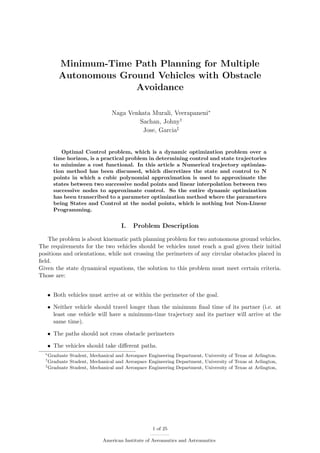
1. Minimum-Time Path Planning for Multiple
Autonomous Ground Vehicles with Obstacle
Avoidance
Naga Venkata Murali, Veerapaneni∗
Sachan, Johny†
Jose, Garcia‡
Optimal Control problem, which is a dynamic optimization problem over a
time horizon, is a practical problem in determining control and state trajectories
to minimize a cost functional. In this article a Numerical trajectory optimiza-
tion method has been discussed, which discretizes the state and control to N
points in which a cubic polynomial approximation is used to approximate the
states between two successive nodal points and linear interpolation between two
successive nodes to approximate control. So the entire dynamic optimization
has been transcribed to a parameter optimization method where the parameters
being States and Control at the nodal points, which is nothing but Non-Linear
Programming.
I. Problem Description
The problem is about kinematic path planning problem for two autonomous ground vehicles.
The requirements for the two vehicles should be vehicles must reach a goal given their initial
positions and orientations, while not crossing the perimeters of any circular obstacles placed in
field.
Given the state dynamical equations, the solution to this problem must meet certain criteria.
Those are:
• Both vehicles must arrive at or within the perimeter of the goal.
• Neither vehicle should travel longer than the minimum final time of its partner (i.e. at
least one vehicle will have a minimum-time trajectory and its partner will arrive at the
same time).
• The paths should not cross obstacle perimeters
• The vehicles should take different paths.
∗
Graduate Student, Mechanical and Aerospace Engineering Department, University of Texas at Arlington.
†
Graduate Student, Mechanical and Aerospace Engineering Department, University of Texas at Arlington,
‡
Graduate Student, Mechanical and Aerospace Engineering Department, University of Texas at Arlington,
1 of 25
American Institute of Aeronautics and Astronautics
2. The differential equations for both the vehicles were given as,
˙xr = V cos φ sin θ
˙yr = V cos φ cos θ
˙θ = (V/L) sin φ
and the constraints for the steering angle is
−π/2 ≤ φ ≤ +π/2
where xr and yr are the cartesian coordinates of the vehicle and θ is the heading angle measured
positive from the vertical y-axis to the body line of the vehicle. The constant, L, is the wheelbase
of the vehicle, and V is the speed.
II. Numerical Trajectory Optimization
A. Direct Collocation:
This section briefly discusses about the direct collocation method which transcribes the dynamic
optimization problem to a nonlinear parameter optimization method. In direct collocation the
entire trajectory is divided into number of nodes called collocation points and a piecewise
continuous functions were used to approximate states and control.The control is approximated
using piecewise continuous linear function and states using piecewise continuous cubics. so the
entire problem now becomes finding the for these piecewise continuous functions which satisfies
the boundary conditions between each successive nodes.
The entire problem is discretized into N number of nodes,
0 = ti < ti+1 < ti+2 < . . . < tN = tf
where, ti, ti+1, . . . , tf are time at Nodes i, i + 1, . . . , N respectively and tf being final time.
The states and controls are also discretized into N parameters at N grid points along with final
time tN , which will be the parameters for nonlinear program.
P = (x(ti), x(ti+1), . . . , x(tN ), u(ti), u(ti+1), . . . , u(tN ), tN )
For each interval from i to i+1 the controls are chosen as piecewise linear interpolating functions,
u(t) = u(ti) +
t − ti
ti+1 − ti
(u(ti+1) − u(ti))
The states are chosen as piecewise continuous cubic polynomials between xi and xi+1,
x(t) = co + c1t + c2t2
+ c3t3
2 of 25
American Institute of Aeronautics and Astronautics
3. To calculate the polynomial coefficients between i and i + 1,
x(ti) = co + c1ti + c2t2
i + c3t3
i (1)
˙x(ti) = c1 + 2c2ti + 3c3t2
i (2)
x(ti+1) = co + c1ti+1 + c2t2
i+1 + c3t3
i+1 (3)
˙x(ti+1) = c1 + 2c2ti+1 + 3c3t2
i+1 (4)
where x(ti), x(ti+1) were obtained from Node points and ˙x(ti), ˙x(ti+1) were obtained from dif-
ferential equations by substituting x(ti), x(ti+1) respectively
So the coefficients were obtained as,
Co
C1
C2
C3
=
1 ti t2
i t3
i
0 1 2ti 3t2
i
1 ti+1 t2
i+1 t3
i+1
0 1 2ti+1 3t2
i+1
−1
∗
x(ti)
˙x(ti)
x(ti+1)
˙x(ti+1)
with boundary conditions xi at ti and xi+1 at ti+1
The approximating functions of the states have to satisfy the differential equations at the grid
points tk, k = 1, . . . , N. This is known as cubic collocation. The assumed approximation of x(t)
must satisfy the differential equations at the grid points tk. As the polynomial already fulfills
the differential equations at the grid points, the only constraints for the nonlinear program will
be,
• the midpoint of the cubic polynomial should be equal to the value of the differential
equation at tc =
(ti+1 − ti)
2
f(x(tc), u(tc), tc) − ˙xc(tc) = 0
which is nothing but the defect at the collocation point and it should be zero,
where ˙xc = c1 + 2c2tc + 3c3t2
c and f(x(tc), u(tc), tc) is differential equation evaluated at
xc =
xi+1 + xi
2
• and all the inequality constraints like obstacles will be added to the nodal points,
g(x(tk), u(tk), tk) ≥ 0, k = 1, . . . , N
• and the initial and end point constraints at t1, tN
Any nonlinear programming technique can be used to solve this problem like sequential quadratic
programming, interior-point method, trust region, active-set.
B. Performance Index:
This section talks about the cost function that should be minimized based on the parameters
and objectives. Those were given as,
• For reaching the goal in minimum time the cost that was used is,
Jf = α1(tf )
where α1 is the weight on the final time, to reduce the emphasis on final time α can be
0.1 or to keep more focus on final time α can be 10 to 25;
3 of 25
American Institute of Aeronautics and Astronautics
4. • To specify the goal position position, the cost function of distance between vehicle and
goal is used,
Jg = α2(x1(tN ) − xg)2
+ (y1(tN ) − yg)2
+ (x2(tN ) − xg)2
+ (y2(tN ) − xg)2
where (xg, yg) are goal location.
• For minimizing the rate of change of control, cost function of minimum control is,
Jc = α3(∆φ2
1 + ∆φ2
2)
• For adding penalty function, when any vehicle violates the obstacle constraint or Vehicle
to Vehicle distance constraint inverse square law is used,
Jp = β/(rj)2
if rj ≤specified distance and
Jp = 0
if rj ≥ given distance.
And β is some weighting term to increase or decrease the penalty term, β = 0.01 to 1 to
increase penalty and β = 1 to 1000 to decrease the penalty.
So the total performance index now becomes,
J = Jf + Jg + Jc + Jp
For the simulation α1 = 1, α2 = 10, α3 = 50, β = 10.
C. Constraints:
This section talks about the constraints on the system that should be added for each node. As
the both vehicles must avoid obstacles, the obstacles were added as constraints at each node for
every obstacle. As the any node can be placed anywhere so each obstacle constraint is given to
each node and it is given as,
g1obstacles =⇒ (rbj)2
− (x1k − xbj)2
+ (y1k − ybj)2
≤ 0
g2obstacles =⇒ (rbj)2
− (x2k − xbj)2
+ (y2k − ybj)2
≤ 0
where, g1obstacles, g2obstacles are obstacle constraint for vehicle 1 and 2 respectively, rbj is the
radius of the obstacle,(xbj, ybj) is the center of obstacles k = 1, . . . , N, j = 1, . . . ,number of
obstacles.
The constraint for maintaining the distance between two vehicles, so that they won’t collide
each other is given as,
gvehicle =⇒ (rvehicle)2
− (x1k − x2k)2
+ (y1k − y2k)2
≤ 0
where rvehicle is the distance between the vehicles that they should maintain.
III. Simulation Setup
The first vehicle is placed at the origin, and the second is placed directly below it at y =
4.Both vehicles are oriented parallel to the x-axis. The minimum allowable distance between
the vehicles is 2.25 units. The vehicle speed is a constant 0.2 units, and the steering wheel may
be deflected up to ±π/2 radians from the axis of the vehicle. Each vehicle has a wheelbase of 2
units. The goal is placed at (25, 15). The safe zone around the goal position is about a radius
2.5 units.
4 of 25
American Institute of Aeronautics and Astronautics
5. IV. Results
This section talks about the results that was obtained from the implementation of above
mentioned technique. The results were divided into two sections, one talks about effect of num-
ber of nodes and another talks about the effect of weight on the minimum control cost.
Effect of Number of nodes:
This section talks about the effect of number of nodes on the overall result without adding the
vehicle to vehicle distance penalty. The increase in number of nodes increases the accuracy of
the result, as the nodes were placed closely together and as cubic polynomial is assumed between
them, the distance between the nodes and the defect is so small, that the defect evaluation at
the mid interval is accurate enough.
The algorithm has been implemented for different number of nodes. It turns out that less
number of nodes were not sufficient enough to consider or avoid obstacles, as the nodes were
spaced far apart from each other, the nodes were not able to see the obstacles. So a good
amount of nodes were required to account for all the obstacles that was given.
5 of 25
American Institute of Aeronautics and Astronautics
6. Figure 1. Obstacle avoidance of two vehicles above one with 37 nodes and below one with 65
nodes
By looking at the fig.1., it turns out that the 37 nodes were actually good enough to avoid
the obstacles. As the two figures (37 nodes and 65 nodes) does look the same, but the result
that was obtained after applying the optimal control which is obtained from the fmincon to
the actual system(differential equations) and integrate the equations forward, the trajectories
of System and Fmincon does not match, which is shown in following figures.
6 of 25
American Institute of Aeronautics and Astronautics
7. Figure 2. Obstacle avoidance of two vehicles with 37 nodes fig.a is the path of the system, and
fig.b is the path from fmincon
From fig.2 it turns out that the paths from the system and fmincon does not match. The
reason for the two paths not matching is because of the steering angle .
7 of 25
American Institute of Aeronautics and Astronautics
8. Figure 3. Steering Angle(Control) of both the vehicles with 37 nodes.
From fig.3 it is clear that there was a lot of jumps of steering angle between the successive
nodes, So because of this reason the solution deviated from the fmincon, after integrating the
system with the obtained Optimal control. This can be rectified by increasing the weight on
the minimum control cost function or by increasing the number of nodes.
8 of 25
American Institute of Aeronautics and Astronautics
9. Figure 4. Obstacle avoidance path of two vehicles from the system and from Fmincon
From fig.4 it turns out that the paths from the system and fmincon does match each other.
It is because of the increasing the number of nodes decreased the jumps between the steering
angle of successive nodes. This was shown in fig.5.
9 of 25
American Institute of Aeronautics and Astronautics
10. Figure 5. Steering Angle(Control) of both the vehicles with 65 nodes.
10 of 25
American Institute of Aeronautics and Astronautics
11. Figure 6. Comparision of Trajectories from System and Fmincon for Vehicle One and Two
11 of 25
American Institute of Aeronautics and Astronautics
12. Figure 7. Comaprision of Heading angle from System and Fmincon for Vehicle one and Two
The fig.6 and fig.8, shows the comparision between Trajectory of states obtained from in-
tegrating the differential equation after obtaining the optimal control and from fmincon for 65
nodes.
12 of 25
American Institute of Aeronautics and Astronautics
13. Effect of weight on Minimum Control cost function:
This section talks about the effect of weight on the Minimum control cost function. Mini-
mum control cost function is the cost function which reduces the rate of change of steering
angle(Control). By increasing the weight on that cost function, the optimizer will reduce that
cost function even further so that corresponding cost function will be much lesser than before
without any weight on it.
So by increasing the weight on the Minimum control cost function will reduce the actuator
rate even further so that we will see smooth curve for Control trajectory.
Figure 8. Obstacle Avoidance of the two vehicles after increasing the weight on the control cost
function to 50 and 67 nodes.
By comparing fig.8 and fig.2 it is clear that after increasing the weight on the control cost
function, we can see that the vehicles path has a lot of curving than from fig.2(No weight on
control). It is because that as the weight decreased the control cost much further, it decreased
the actuator rates so the vehicles don’t have much of an option to turn instantaneously as
before. But adding weight on the control also increases the final time. As the vehicle have to
take longer turn than before, the final time increased a lot than before. Final time with no
weight on control cost function came out to be 177.74 seconds and after adding the weight on
the control the final time turns out to be 235.5138 seconds.
13 of 25
American Institute of Aeronautics and Astronautics
14. Figure 9. Comparision of Trajectories of both the vehicles with System and Fmincon with 67
nodes
14 of 25
American Institute of Aeronautics and Astronautics
15. Figure 10. Comparision of Trajectories of Heading angle for both the vehicles with System and
Fmincon with 67 nodes
15 of 25
American Institute of Aeronautics and Astronautics
16. Figure 11. Steering angle of both the vehicles with 67 nodes
By looking at the fig.11(weight on control) and fig.5(No weight on control) it looks like fig.5
have lesser oscillations than fig.11. But by looking at the difference in angle φ(tf ) − φ(t0) it
turns out that the δφ for fig.5 is 30o compared to δφ for fig.11 which is 18o.
16 of 25
American Institute of Aeronautics and Astronautics
17. After adding Penalty for Vehicle to Vehicle distance constraint:
This section talks about the obstacle avoidance path after adding the Vehicle to Vehicle dis-
tance penalty function. The simulation is conducted with 67 nodes by adding the inequality
constraints for Vehicle to Vehicle distance maintenance. Penalty function is introduced into the
cost function for violations of the vehicle to vehicle distance constraint with weight on Penalty
100. The constraint was removed when the rover is 5 units within the goal position. The
following were the results obtained after implementing this simulation case,
Figure 12. Comparision of Obstacle avoidance path of two rovers between system (After integrat-
ing) and Fmincon with 67 nodes and 10 weight on Minimum Control Cost.
From the above figure, it turns out that the Fmincon violated the Vehicle to Vehicle con-
straints with penalty function, but the actual system tends to maintain some distance between
two vehicles.
17 of 25
American Institute of Aeronautics and Astronautics
18. Figure 13. Comparision of Trajectory of two rovers between system (After integrating) and
Fmincon with 67 nodes and 10 weight on Minimum Control Cost.
18 of 25
American Institute of Aeronautics and Astronautics
19. Figure 14. Comparision of Trajectory of Heading angle of two rovers between system (After
integrating) and Fmincon with 67 nodes and 10 weight on Minimum Control Cost.
19 of 25
American Institute of Aeronautics and Astronautics
20. Figure 15. Trajectory of steering angle(Control) of two rovers with 67 nodes and no weight on
Minimum Control Cost.
With different Initial Conditions:
This section talks about the what the algorithm tries to do if one vehicle is close to the goal
and another vehicle is far apart. The position of rover one is changed to (30,15) just 5 units
beside the goal and the rover two position is at (0,-4). It is expected that the vehicle close to
the goal has to travel away from goal and come back to achieve the minimum time, same time
20 of 25
American Institute of Aeronautics and Astronautics
21. condition.
The following figure demonstrates the above mentioned result.
Figure 16. Comparision of Obstacle Avoidance Trajectory of both vehicles obtained from sys-
tem(Intgeration) and Fmincon
From the above figure, it is clear that because the first vehicle is close to goal and it cannot
reach the goal before the second obstacle it did deviated from the goal position went through
all the unnecessary path and then both the vehicles reached the goal position at the same time.
21 of 25
American Institute of Aeronautics and Astronautics
22. Both the trajectories did not matched perfectly because when we integrate the system with a
step size of 0.1 the path kind of deviated because of the lot of jumps in steering angle. As
this simulation is done without using any weight on the control, this can be rectified by adding
weight on the Minimum control cost function.
Figure 17. Trajectory of both vehicles obtained from system(Intgeration) and Fmincon
22 of 25
American Institute of Aeronautics and Astronautics
23. Figure 18. Trajecttory of Heading angle for both the rover’s system and fmincon
23 of 25
American Institute of Aeronautics and Astronautics
24. Figure 19. Trajectory of steering angle of both the vehicles
24 of 25
American Institute of Aeronautics and Astronautics
25. V. Team Member Contributions to project
Team Member Contribution(%)
V.N.V.Murali 80
Sachan,Johny 10
Jose,Garcia 10
VI. Conclusion
From the above mentioned technique and results the direct collocation method is flexible
enough to handle complex problems. The solution accuracy of this collocation method can be
improved much further by using orthogonal polynomials to approximate the state and control
trajectories instead of using cubic polynomials to approximate and this method of approximation
is called orthogonal collocation. The same technique can be used for path planning of vehicles
in dynamic obstacles environment. While collocation is good it takes much longer to converge
as the better solution needs more number of nodes, and this collocation technique cannot be
implemented in real-time, atleast not with Fmincon.
References
1. Oskar von Stryk,”Numerical Solution of Optimal Control Problems by Direct Collocation”,
Calculus of Variations, Optimal Control Theory and Numerical Methods, International
Series of Numerical Mathematics, Vol. 111, p.129-143, Birkhauser, 1993
2. Oskar von Stryk and R. Bulirsch, ”Direct and Indirect Methods for Trajectory Optimiza-
tion”, Mathematisches Institut, Technische Universitat Munchen, Postfach 20 24 20, D-
8000 Munchen 2, Germany.
25 of 25
American Institute of Aeronautics and Astronautics