Downloaded 10 times
![International Journal of Electronics and Communication Engineering & Technology (IJECET), ISSN
INTERNATIONAL JOURNAL OF ELECTRONICS AND
0976 – 6464(Print), ISSN 0976 – 6472(Online) Volume 3, Issue 1, January- June (2012), © IAEME
COMMUNICATION ENGINEERING & TECHNOLOGY (IJECET)
ISSN 0976 – 6464(Print)
ISSN 0976 – 6472(Online)
Volume 3, Issue 1, January- June (2012), pp. 98-110
IJECET
© IAEME: www.iaeme.com/ijecet.html
Journal Impact Factor (2011): 0.8500 (Calculated by GISI) ©IAEME
www.jifactor.com
FAST DCT ALGORITHM USING WINOGRAD’S METHOD
Ch. Ramesh1, Dr.N.B. Venkateswarlu2, Dr. J.V.R. Murthy3
1
Professor, Dept .of CSE, AITAM, Tekkali, A.P, India
chappa_ramesh01@yahoo.co.in
2
Professor, Dept .of CSE, AITAM, Tekkali, A.P, India
venkat_ritch@yahoo.com
3
Professor, Dept .of CSE, College of Engineering, JNTUK, A.P, India
mjonnalagedda@yahoo.com
ABSTRACT
Applications of Digital Image Communication have increased exponentially in the
recent years. Evidently, discrete cosine transform (DCT) based algorithms are in wide
use for reducing communication cost. Forward DCT and inverse DCT computation
are reported to be taking very long time which may often impede real time responses
in some applications. In this paper, we present Winograd’s matrix multiplication
approach for forward DCT and inverse DCT computation to reduce their CPU time.
Experiments are made with standard images and synthetic images.
Key Words: DCT, IDCT, Winograd’s, JPEG, MATLAB
I. INTRODUCTION
Discrete cosine transform (DCT) based algorithms such as JPEG, JPEG2000, MP3,
are the most widely used in the audio, image, and video data compression. DCT is
originally developed by Ahmed, Natarajan, and Rao (1974). Its application to image
compression was pioneered by Chen and Pratt (1984). DCT is a technique for
converting a signal into elementary frequency components. DCT represents an image
as a sum of sinusoids of varying magnitudes and frequencies.
The DCT has the property that, for a typical image, most of the visually significant
information about the image is concentrated in just a few coefficients of the DCT, for
this reason the DCT is often used in image compression applications [3]. The cosines
transform converts each block of spatial information into an efficient frequency space
representation that is better suited for compression. Specifically, the transform
produces an array of coefficients for real-valued basis functions that represent each
block of data in frequency space. The magnitude of the DCT coefficients exhibits a
distinct pattern within the array, where transform coefficients corresponding to the
98](https://image.slidesharecdn.com/fastdctalgorithmusingwinogradsmethod-121125011541-phpapp02/85/Fast-dct-algorithm-using-winograd-s-method-1-320.jpg)
![International Journal of Electronics and Communication Engineering & Technology (IJECET), ISSN
INTERNATIONAL JOURNAL OF ELECTRONICS AND
0976 – 6464(Print), ISSN 0976 – 6472(Online) Volume 3, Issue 1, January- June (2012), © IAEME
COMMUNICATION ENGINEERING & TECHNOLOGY (IJECET)
ISSN 0976 – 6464(Print)
ISSN 0976 – 6472(Online)
Volume 3, Issue 1, January- June (2012), pp. 98-110
IJECET
© IAEME: www.iaeme.com/ijecet.html
Journal Impact Factor (2011): 0.8500 (Calculated by GISI) ©IAEME
www.jifactor.com
FAST DCT ALGORITHM USING WINOGRAD’S METHOD
Ch. Ramesh1, Dr.N.B. Venkateswarlu2, Dr. J.V.R. Murthy3
1
Professor, Dept .of CSE, AITAM, Tekkali, A.P, India
chappa_ramesh01@yahoo.co.in
2
Professor, Dept .of CSE, AITAM, Tekkali, A.P, India
venkat_ritch@yahoo.com
3
Professor, Dept .of CSE, College of Engineering, JNTUK, A.P, India
mjonnalagedda@yahoo.com
ABSTRACT
Applications of Digital Image Communication have increased exponentially in the
recent years. Evidently, discrete cosine transform (DCT) based algorithms are in wide
use for reducing communication cost. Forward DCT and inverse DCT computation
are reported to be taking very long time which may often impede real time responses
in some applications. In this paper, we present Winograd’s matrix multiplication
approach for forward DCT and inverse DCT computation to reduce their CPU time.
Experiments are made with standard images and synthetic images.
Key Words: DCT, IDCT, Winograd’s, JPEG, MATLAB
I. INTRODUCTION
Discrete cosine transform (DCT) based algorithms such as JPEG, JPEG2000, MP3,
are the most widely used in the audio, image, and video data compression. DCT is
originally developed by Ahmed, Natarajan, and Rao (1974). Its application to image
compression was pioneered by Chen and Pratt (1984). DCT is a technique for
converting a signal into elementary frequency components. DCT represents an image
as a sum of sinusoids of varying magnitudes and frequencies.
The DCT has the property that, for a typical image, most of the visually significant
information about the image is concentrated in just a few coefficients of the DCT, for
this reason the DCT is often used in image compression applications [3]. The cosines
transform converts each block of spatial information into an efficient frequency space
representation that is better suited for compression. Specifically, the transform
produces an array of coefficients for real-valued basis functions that represent each
block of data in frequency space. The magnitude of the DCT coefficients exhibits a
distinct pattern within the array, where transform coefficients corresponding to the
98](https://image.slidesharecdn.com/fastdctalgorithmusingwinogradsmethod-121125011541-phpapp02/75/Fast-dct-algorithm-using-winograd-s-method-1-2048.jpg)
![International Journal of Electronics and Communication Engineering & Technology (IJECET), ISSN
0976 – 6464(Print), ISSN 0976 – 6472(Online) Volume 3, Issue 1, January- June (2012), © IAEME
lowest frequency basis functions usually have the highest magnitude and are the most
perceptually significant. Similarly, discrete cosine transform coefficients
corresponding to the highest frequency basis functions usually have the lowest
magnitude and are the least perceptually significant. In DCT based compression
methods, only important DCT coefficients are retained. Thus, we achieve
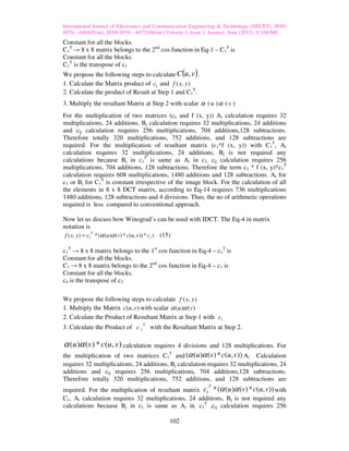
compression of data.
The 2D-DCT equation (Eq-1) computes the u, v th entry of the DCT of an image [5]
( 2 x + 1)uπ
N −1 N −1
(2 y + 1)vπ for u, v = 0, 1, 2 …….N-1 (1)
C (u, v ) = α (u )α (v)∑∑ f ( x, y ) cos cos
x =0 y =0 2N 2N
1/ N for u = 0
α (u ) = (2)
2/ N for u > 0
1/ N for u = 0
α (v ) = (3)
2/ N for u > 0
f (x, y) is the x, yth element of the image represented by the matrix f. N is the size of
the block that the DCT is done on. The equation calculates one entry (u, vth) of the
transformed image from the pixel values of the original image matrix.
The first coefficient C00 is termed the “DC coefficient” and the remaining coefficients
are called the “AC coefficients”. After performing DCT, the remaining operations at
the sender side are quantization, zigzag and encoding. The reverse operations at the
receiving side are decoding, inverse zigzag, de-quantization and IDCT. As these
concepts are widely reported elsewhere, we skip discussion about them for the
reasons of terseness.
The IDCT is a transform that converts a set of frequency coefficients to a signal for an
image, this transform is performed on a 2 dimensional array of coefficients resulting
in a 2 dimensional array of samples.
The 2D-IDCT equation (Eq-4) computes the x, yth entry of an image. [5]
N −1 N −1
(2 x + 1)uπ (2 y + 1)vπ (4)
f ( x, y ) = ∑∑α (u )α (v)C (u, v) cos cos 2 N
u =0 v =0 2N
for x, y = 0, 1, 2 …….N-1
C (u, v) is u, vth DCT coefficient of the image represented by the matrix C. N is the
size of the block that the IDCT is done on. The equation calculates one entry (x, yth)
of the image from the transformed coefficients of the IDCT matrix.
This paper is organized as follows. In section II, we have given a brief overview of
DCT and IDCT algorithms by conventional approach . The proposed Winograd’s
based DCT and IDCT algorithms are described in section III. Experimental results are
presented in IV. Finally, concluding remarks are given in section V.
II. Computational Complexity of Conventional DCT/IDCT
99](https://image.slidesharecdn.com/fastdctalgorithmusingwinogradsmethod-121125011541-phpapp02/85/Fast-dct-algorithm-using-winograd-s-method-2-320.jpg)
![International Journal of Electronics and Communication Engineering & Technology (IJECET), ISSN
0976 – 6464(Print), ISSN 0976 – 6472(Online) Volume 3, Issue 1, January- June (2012), © IAEME
(2 x + 1)uπ
In the 2D-DCT (Eq-1) the cosine functions cos and
2N
(2 y + 1)vπ (2 y + 1)vπ
cos are computationally very expensive. cos is the transpose
2N 2N
(2 x + 1)uπ (2 x + 1)uπ
of cos . Calculation of cos requires 4 multiplications, 1
2N 2N
addition, and 1 division. For calculation of each element in DCT matrix the loop in
(2 x + 1)uπ
Eq-1 iterates 64 times. Therefore cos requires 256 multiplications, 64
2N
additions and 64 divisions. For calculation of all elements in DCT matrix, it requires
16384 multiplications 4096 additions and 4096 divisions. Therefore both the cos
functions require 32768 multiplications 8192 additions and 8192 divisions. Therefore
the way to improve the performance is to pre compute the coefficients and read them
during DCT algorithms. In this way for the calculation of each element in DCT
matrix, the Eq-1 requires 130 multiplications, 63 additions and 2 divisions. Similarly
for the calculation of all the elements in 8x8 DCT matrix The Eq-1 requires 8320
multiplications,4023 additions and 2 divisions. For the calculation of each element in
IDCT matrix, the Eq-4 requires 256 multiplications, 63 additions and 2 divisions.
Similarly for the calculation of all the elements in 8x8 IDCT matrix The Eq-4
requires 16384 multiplications, 4023 additions and 2 divisions. The IDCT requires
more number of arithmetic operations compared to DCT.
III. Winograd’s Approach
Consider calculation of scalar or dot product of two vectors, X and Y
X = [x1, x2, …..xN] (5)
Y = [y1, y2,…...yN] (6)
T
X Y= x1y1 +x2y2+ …+xNyN (7)
This calculation usually requires N multiplications and N additions. Winograd’s
algorithm [2, 5] is used in the literature to reduce these computations in applications
such as classification, etc. According to [2],
XTY= [(x1+y2)(x2+y1)+(x3+y4)(x4+y3) + …. + (xN+yN-1)(xN-1+yN) ] –
[ x1x2+x3x4+ … xN-1xN] –
[ y1y2 + y3y4 + …. + yN-1yN] (8)
This can be also represented as below assuming k=N/2.
2k k (9) k k
X T Y = ∑xi yi = ∑( x2u −1 + y2u )(x2u + y2u −1 ) − ∑x2u x2u −1 − ∑y2u y2u −1
i =1 u =1 u =1 u =1
By representing in the above form, if last two terms are assumed to be pre-calculated,
we can get dot product with N/2 multiplications itself. In some applications, last two
terms can be re-used. Thus, we may get computational benefit. This theme we
propose to use in our DCT/IDCT algorithm’s by extending this to matrix
multiplication. Of course, here we have assumed N is even number, thus N/2 pairs are
available. If N is not even, we can simply convert X and Y into even by adding one 0
at the end.
Though Winograd’s algorithm [2, 5] reduces actual computations involved, its
asymptotic computational complexity is same as the naïve matrix multiplication
100](https://image.slidesharecdn.com/fastdctalgorithmusingwinogradsmethod-121125011541-phpapp02/85/Fast-dct-algorithm-using-winograd-s-method-3-320.jpg)
![International Journal of Electronics and Communication Engineering & Technology (IJECET), ISSN
0976 – 6464(Print), ISSN 0976 – 6472(Online) Volume 3, Issue 1, January- June (2012), © IAEME
algorithm. In our DCT algorithm, we are required to carry a series of matrix
multiplications. We propose to reduce CPU time requirements by meticulously using
Winograd’s method.
For the multiplication of two N x N square matrices A and B Winogard’s algorithm is
defined as shown in equations (11), (12) and (13) below.
Ci,j=Product of Ai and Bj (10)
n/2
Ci , j = ∑ ( ai , 2 K −1 + b2 K , j )(ai , 2 K + b2 K −1, j ) − Ai − B j
(11)
K =1
n/2
Ai = ∑ ai , 2 K −1 .a i , 2 K (12)
K =1
n/2
B j = ∑ b2 K −1, j .b2 K , j (13)
K =1
Ai → Sum of pairwise multiplication of couples in ith row.
B j → Sum of pairwise multiplication of couples in jth column.
Ci , j → ith row, jth column element of matrix C.
Since Ai and Bj are pre-computed once for each row of A and column of B. They
require only N2 multiplications. That is, to calculate pair-wise product of any row or
column of N x N matrix, we need N/2 multiplications. For N rows or columns, we
need NxN/2 multiplications. Thus, in total to calculate pair-wise product of rows of A
and columns of B, we need N2 multiplications. The total number of multiplications
1 3
needed to calculate matrix product becomes: N + N 2 . However, the number of
2
3
additions and subtractions has been increased to ( ) N 3 + 2 N 2 − 2 N .Winograd’s
2
algorithm is theoretically faster than the naïve matrix multiplication algorithm,
because additions takes very less CPU time compared to multiplications. In DCT or
IDCT computations matrices are of size 8 x 8. For an 8x8 matrix, each Ai calculation
requires 4 multiplications, 3 additions. Each B j calculation requires 4
multiplications, 3 additions. Each Ci , j calculation requires 4 multiplications, 3
additions and 2 subtractions. For multiplication of two 8x8 matrices 320
multiplications, 752 additions and 128 subtractions are required.
Now let us discuss how Winograd’s matrix multiplication method can be used with
DCT. The Eq-1 in matrix notation can be represented as [12]
T
C (u, v ) = α (u )α (v) * (c1 * f ( x, y) * c1 ) (14)
f (x, y) → 8 x 8 image block
c1 → 8 x 8 matrix belongs to the 1st cos function in Eq-1 – c1 is
101](https://image.slidesharecdn.com/fastdctalgorithmusingwinogradsmethod-121125011541-phpapp02/85/Fast-dct-algorithm-using-winograd-s-method-4-320.jpg)
![International Journal of Electronics and Communication Engineering & Technology (IJECET), ISSN
0976 – 6464(Print), ISSN 0976 – 6472(Online) Volume 3, Issue 1, January- June (2012), © IAEME
multiplications, 704 additions, 128 subtractions. For the calculation of all the
elements in 8 x 8 DCT matrix, according to Eq-15 requires 736 multiplications 1480
additions, 128 subtractions and 4 divisions. The total no of arithmetical operations
required is less when compared to conventional approach.
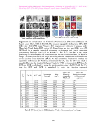
IV. EXPERIMENTAL WORK
In this study a number of images in tiff format are used including the widely used
Lena, Mandrill and Pepper images. The Table-1 shows the complete details of images
used in our study.
S. No Fig No Image Size Type
1 1(a) Chess 128x128 Gray
2 1(b) Helmet 128x128 Gray
3 1(c) X-ray 128x128 Gray
4 1(d) Clock 256x256 Gray
5 1(e) Moon surface 256x256 Gray
6 1(f) Cameraman 256x256 Gray
7 1(g) Lena 512x512 Gray
8 1(h) Mandrill 512x512 Gray
9 1(i) Peppers 512x512 Gray
10 1(j) Man 1024x1024 Gray
11 1(k) Airplane2 1024x1024 Gray
12 1(l) Airport 1024x1024 Gray
13 1(m) Flowers 2048x2048 Gray
14 1(n) Flowers1 2048x2048 Gray
15 1(0) City 2048x2048 Gray
16 2(a) Couple 128x128 Color
17 2(b) House 128x128 Color
18 2(c) Jennybeans1 128x128 Color
19 2(d) Girl1 256x256 Color
20 2(e) Jennybeans 256x256 Color
21 2(f) Tree 256x256 Color
22 2(g) Girl2 512x512 Color
23 2(h) Sailboat 512x512 Color
24 2(i) Splash 512x512 Color
25 2(j) Oakland 1024x1024 Color
26 2(k) Richmond 1024x1024 Color
27 2(l) Shreport 1024x1024 Color
28 2(m) Flowers 2048x2048 Color
29 2(n) Flowers1 2048x2048 Color
30 2(0) City 2048x2048 Color
Table 1: Details of images used in our study
All the above images are taken from the USC-SIPI image database
“http://sipi.usc.edu/database” [6]
103](https://image.slidesharecdn.com/fastdctalgorithmusingwinogradsmethod-121125011541-phpapp02/85/Fast-dct-algorithm-using-winograd-s-method-6-320.jpg)
![International Journal of Electronics and Communication Engineering & Technology (IJECET), ISSN 0976 –
6464(Print), ISSN 0976 – 6472(Online) Volume 3, Issue 1, January- June (2012), © IAEME
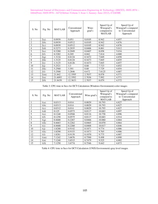
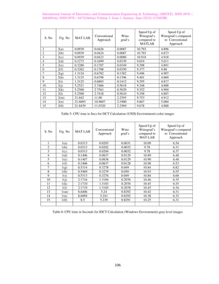
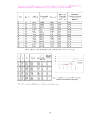
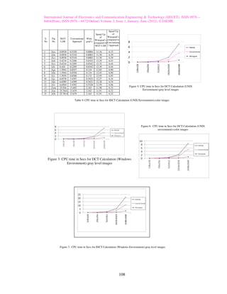
conventional algorithm. We are getting a speed up of more than 10 when compared
to MATLAB and more than 6 when compared to conventional algorithm.
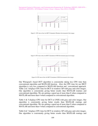
Table 8 & 9 displays CPU time for DCT in windows XP with gray and color images.
Our algorithm is consistently giving better results than MATLAB routings and
conventional algorithm. We are getting a speed up of more than 11 when compared
to MATLAB and more than 6 when compared to conventional algorithm.
The CPU time for DCT and IDCT calculations for the color images is around 3 times
for the corresponding size gray level image.
The Speedup of CPU time for DCT and IDCT calculations in UNIX environment as
compared to CPU time for DCT and IDCT calculations in Windows environment is
around 15%.
V. CONCLUSIONS
In this paper, Winograd based fast DCT and IDCT algorithms were proposed. We
have compared our DCT and IDCT algorithms with conventional, MATLAB
counterparts. From our experiments it is evident that our Winograd’s based DCT and
IDCT algorithms is the most preferred algorithms as they consume very less CPU
time compared to conventional implementation and MATLAB. Our approach can be
employed to compress video sequences also.
REFERENCES
[1]N.BVenkateswarlu and P.S.V.S.K.Raju “Winograd’s method:A perspective for some
pattern recognition problems” 105-109,Vol 15 ,No2,1994 Pattern Recognition
Letters.
[2]N.BVenkateswarlu and P.S.V.S.K.Raju “Winograd’s Inequality:A perspective for
some PR problems”, Pattern Recognition Letters 1991.
[3]R.C.Gonzalez and R.E.Woods “Digital Image Processing”,2nd Edition Addison
Wesley,USA ISBN:0-201-60078,1993
[4]The USC–SIPI image database (http://sipi.usc.edu/database).Signal and image
processing institute Ming Hgieh Department of Electrical Engineering..
[5]Rudra Pratap “Getting started with Matlab”:A Quick Introduction for Scientist and
Engineer” version 6 Oxford university press 2003.
[6]Andrew B.Watson “Image Compression using the discrete cosine transform”
Mathematica Journal 4(1),1994, p-81-88
[7]D.L.Lee and M.A.Aboelaze “Linear speedup of Winograd’s matrix multiplication
algorithm using an array processor”. Distributed memory computing conference,1991
proceedings of IEEE,pages(427-430).
[8]R.P.Bent “Algorithms for matrix multiplication”,Technical report TR-CS-70-
157,DCS,Stanford University (March 1970).
[9]Boyko Kakaradov “Ultra-fast Matrix Multiplication:An Empirical Analysis of
Highly optimized vector Algorithms“, Stanford under graduate Research journal
2004
[10]Ken cabeen and peter gent,”Image compression and the discrete cosine
transform”,Math 45 college of redwoods
110](https://image.slidesharecdn.com/fastdctalgorithmusingwinogradsmethod-121125011541-phpapp02/85/Fast-dct-algorithm-using-winograd-s-method-13-320.jpg)

This document discusses fast algorithms for computing the discrete cosine transform (DCT) and inverse discrete cosine transform (IDCT) using Winograd's method. The conventional DCT and IDCT algorithms have high computational complexity due to cosine functions. Winograd's algorithm reduces the number of multiplications required for matrix multiplication by rearranging terms. The document proposes applying Winograd's algorithm to DCT and IDCT computation by representing the transforms as matrix multiplications. This approach reduces the number of multiplications required for an 8x8 block from over 16,000 to just 736 multiplications, with fewer additions and subtractions as well. This leads to faster DCT and IDCT computation compared


![2.[9 17]comparative analysis between dct & dwt techniques of image compression](https://cdn.slidesharecdn.com/ss_thumbnails/2-9-17comparativeanalysisbetweendctdwttechniquesofimagecompression-111203184847-phpapp01-thumbnail.jpg?width=640&height=640&fit=bounds)
![2.[9 17]comparative analysis between dct & dwt techniques of image compression](https://cdn.slidesharecdn.com/ss_thumbnails/2-9-17comparativeanalysisbetweendctdwttechniquesofimagecompression-111125091140-phpapp01-thumbnail.jpg?width=640&height=640&fit=bounds)