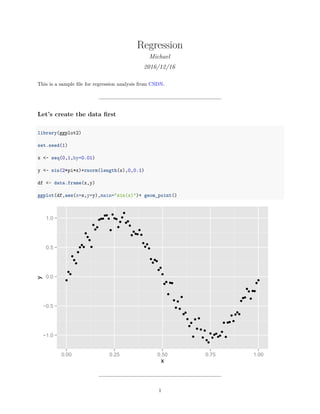
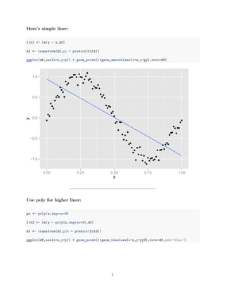
1) The document describes performing regression analysis on simulated sine wave data to compare different regression models. Simple linear regression, polynomial regression with degrees 3 and 26, and regularized regression using l1, l2, and cross-validation are examined. 2) Cross-validation is used to compare train and test RMSE for polynomial models of degrees 1-10, showing higher degree does not necessarily yield better performance. 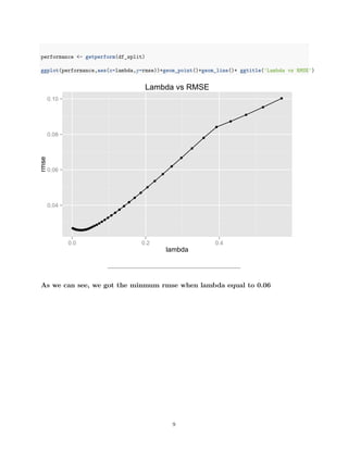3) Regularization methods like l1 norm, l2 norm, and selecting lambda via cross-validation are explored, with the best lambda found to be 0.06 based on minimizing test RMSE.

1. Regression
Michael
2016/12/16
This is a sample file for regression analysis from CSDN.
Let’s create the data first
library(ggplot2)
set.seed(1)
x <- seq(0,1,by=0.01)
y <- sin(2*pi*x)+rnorm(length(x),0,0.1)
df <- data.frame(x,y)
ggplot(df,aes(x=x,y=y),main="sin(x)")+ geom_point()
−1.0
−0.5
0.0
0.5
1.0
0.00 0.25 0.50 0.75 1.00
x
y
1

2. Here’s simple liner:
fit1 <- lm(y ~ x,df)
df <- transform(df,yy = predict(fit1))
ggplot(df,aes(x=x,y=y)) + geom_point()+geom_smooth(aes(x=x,y=yy),data=df)
−1.0
−0.5
0.0
0.5
1.0
0.00 0.25 0.50 0.75 1.00
x
y
Use poly for higher liner:
po <- poly(x,degree=3)
fit3 <- lm(y ~ poly(x,degree=3),df)
df <- transform(df,yy3 = predict(fit3))
ggplot(df,aes(x=x,y=y)) + geom_point()+geom_line(aes(x=x,y=yy3),data=df,col='blue')
2

3. −1.0
−0.5
0.0
0.5
1.0
0.00 0.25 0.50 0.75 1.00
x
y
Enhance the poly:
fit26 <- lm(y ~ poly(x,degree=26),df)
df <- transform(df,yy26 =predict(fit26))
ggplot(df,aes(x=x,y=y)) + geom_point()+geom_line(aes(x=x,y=yy26),data=df,col='blue')
3

4. −1.0
−0.5
0.0
0.5
1.0
0.00 0.25 0.50 0.75 1.00
x
y
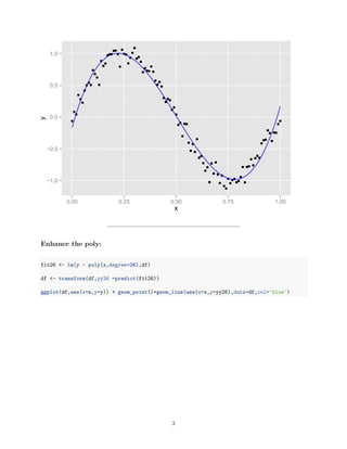
Higher poly doesn’t enjoy better performance, we use RMSE to cross-validation
model:
#Create rmse function:
rmse <- function(y,ry)
{
return(sqrt(sum((y-ry)^ 2))/length(ry))
}
#Create split function for cross-validation
split <- function(df,rate)
{
n <- length(df[,1])
index <- sample(1:n,round(rate * n))
train <- df[index,]
test <- df[-index,]
df <- list(train=train,test=test,data=df)
4

5. return(df)
}
#Create function to plot output
performance_Gen <- function(df,n){
performance <- data.frame()
for(index in 1:n){
fit <- lm(y ~ poly(x,degree=index),data = df$train)
performance <- rbind(performance,data.frame(degree =index,type='train',rmse=rmse(df$train['y'],predic
performance <- rbind(performance,data.frame(degree = index,type='test',rmse=rmse(df$test['y'],predict
}
return(performance)
}
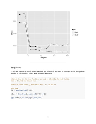
Plot output about train & test dataset:
df_split <- split(df,0.5)
performance<- performance_Gen(df_split,10)
ggplot(performance,aes(x=degree,y=rmse,linetype=type))+geom_point()+geom_line()
5

6. 0.02
0.04
0.06
2.5 5.0 7.5 10.0
degree
rmse
type
train
test
Regularize
After we created a model and it fits well for currently, we need to consider about the perfor-
mance in the further, that’s why we need regularize
#lambda here is the loss function, we need to identify the best lambda
#so as to find the minmum rmse
#There's three kinds of regularize here, l1, l2 and l3
#l1 norm
l1 <- abs(sort(coef(fit3)))
df_l1 <-data.frame(x=sort(coef(fit3)),y=l1)
ggplot(df_l1,aes(x=x,y=y))+geom_line()
6

7. 0
2
4
−5.0 −2.5 0.0 2.5
x
y
#l2 norm
l2 <- (coef(fit3)^2)
df_l2 <-data.frame(x=sort(coef(fit3)),y=l2)
ggplot(df_l2,aes(x=x,y=y))+geom_smooth()+ggtitle('L2norm')
7

8. −200
−100
0
100
200
−5.0 −2.5 0.0 2.5
x
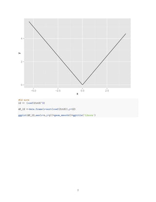
y L2norm
#Use cross-validation to find the best lambda
library(glmnet)
getperform <- function(df){
fit<- with(df$train,glmnet(poly(x,degree=10),y))
lambdas <- fit$lambda
performance <- data.frame()
for( lambda in lambdas){
performance <- rbind(performance,data.frame(
lambda=lambda,
rmse=rmse(df$test['y'],with(df$test,predict(fit,poly(x,degree=10),s=lambda)))))
}
return(performance)
}
8

9. performance <- getperform(df_split)
ggplot(performance,aes(x=lambda,y=rmse))+geom_point()+geom_line()+ ggtitle('Lambda vs RMSE')
0.04
0.06
0.08
0.10
0.0 0.2 0.4
lambda
rmse
Lambda vs RMSE
As we can see, we got the minmum rmse when lambda equal to 0.06
9