- The document examines flaws in the experimental design and methodology of the paper "Debunking the Myths of Influence Maximization: A Benchmarking Study". - It identifies fundamental flaws that lead to incorrect conclusions, such as algorithms being held to different standards of optimality. - It also finds unreproducible and critical experiments used to determine benchmarking parameters, and refutes over 10 misclaims made about previous influence maximization algorithms.

1. Refutations on “Debunking the Myths of
Influence Maximization: A Benchmarking Study”
Wei Lu (Rupert Labs), Xiaokui Xiao (Nanyang Technological Univ.),
Amit Goyal (Google), Keke Huang (Nanyang Technological Univ.),
Laks V.S. Lakshmanan (UBC)
https://arxiv.org/abs/1705.05144

2. Background & Overview
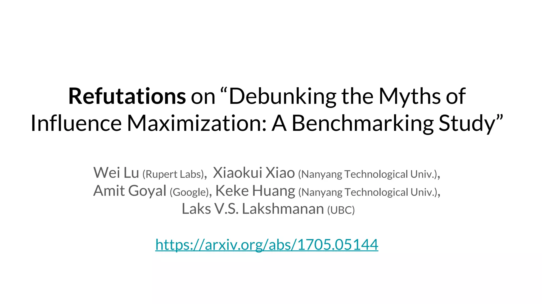
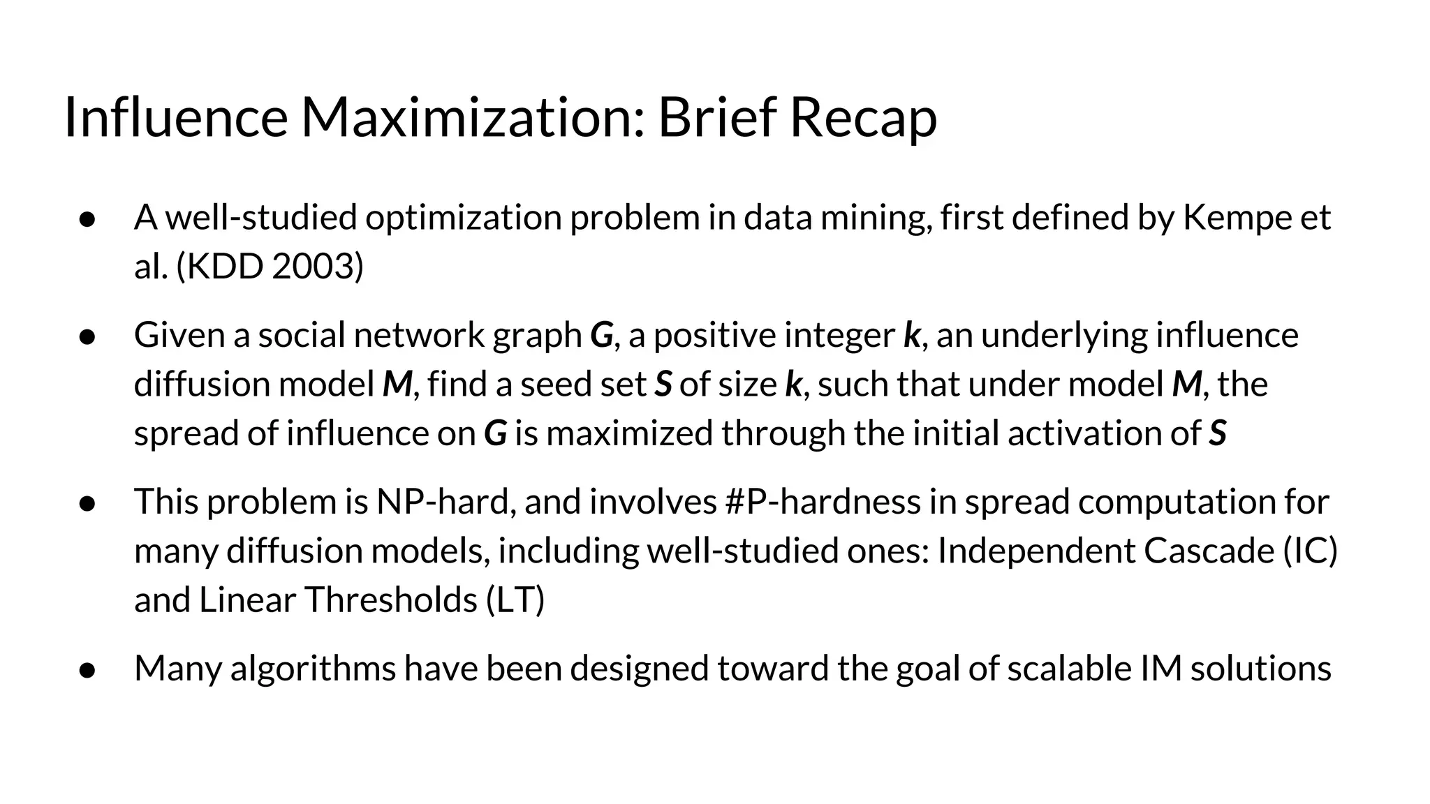
● “Debunking the Myths of Influence Maximization: A Benchmarking Study” [1] is a
SIGMOD 2017 paper by Arora, Galhotra, and Ranu. That paper:
○ undertakes a benchmarking performance study on the problem of Influence
Maximization
○ claims to unearth and debunks many “myths” around Influence Maximization
research over the years
● Our article (https://arxiv.org/abs/1705.05144 ):
○ examines fundamental flaws of their experimental design & methodology
○ points out unreproducible result in critical experiments
○ refutes 11 mis-claims in [1]

3. Our goals and contributions
● Objectively, critically, and thoroughly review Arora et al. [1]
● Identify fundamental flaws in [1]’s experimental design/methodology, which:
○ fails to understand the trade-off between efficiency and solution quality
○ when generalized, leads to obviously incorrect conclusions such as the
Chebyshev’s inequality is better than Chernoff bound
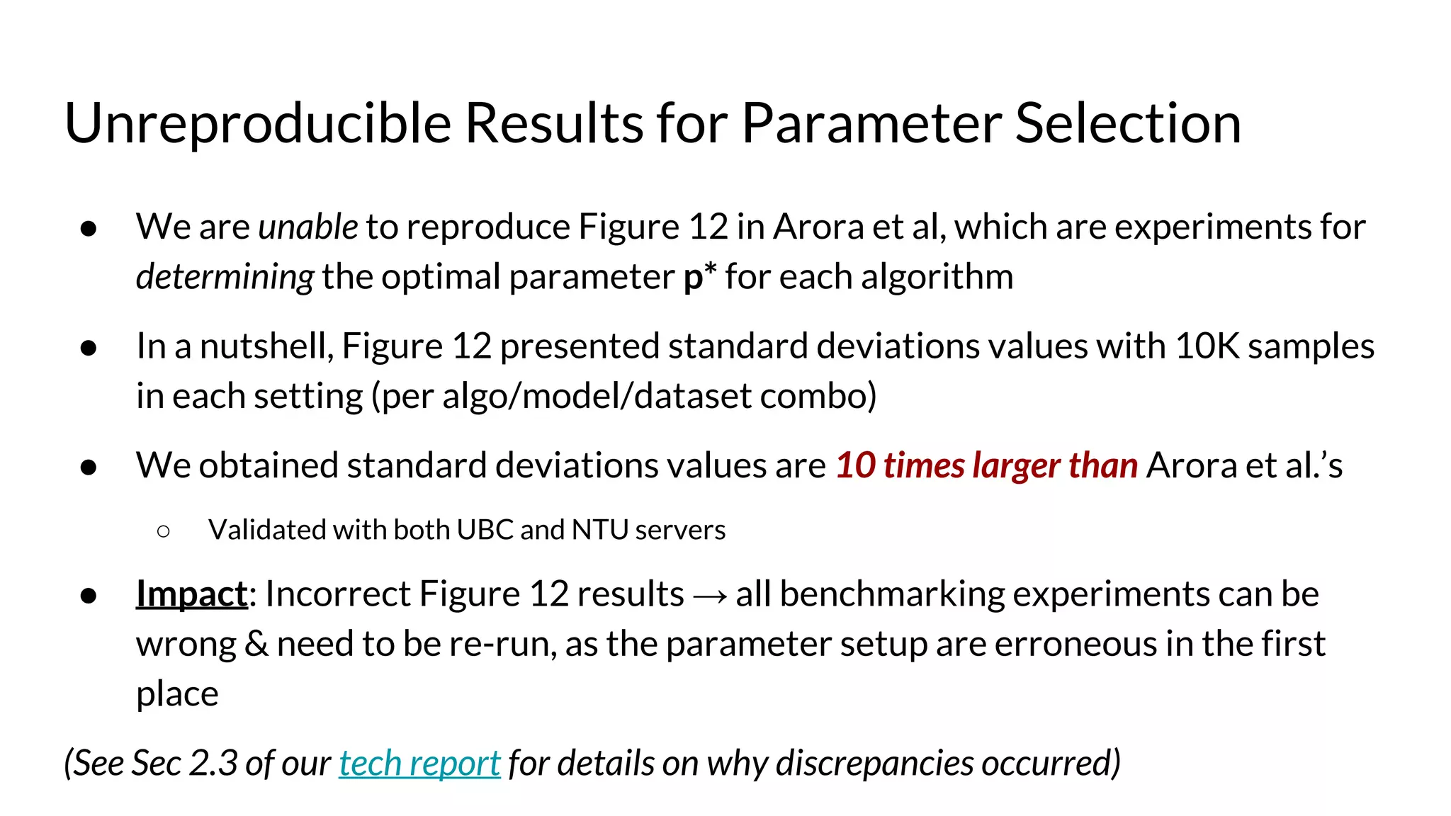
● Identify unreproducible, but critical experiments which are used to determine
benchmarking parameters. By design, this has serious implications of the
correctness of all experiments in Arora et al. [1]
● Refute 11 mis-claims by Arora et al. [1] on previously published papers,
including then state-of-the-art approximation algorithms

4. Influence Maximization: Brief Recap
● A well-studied optimization problem in data mining, first defined by Kempe et
al. (KDD 2003)
● Given a social network graph G, a positive integer k, an underlying influence
diffusion model M, find a seed set S of size k, such that under model M, the
spread of influence on G is maximized through the initial activation of S
● This problem is NP-hard, and involves #P-hardness in spread computation for
many diffusion models, including well-studied ones: Independent Cascade (IC)
and Linear Thresholds (LT)
● Many algorithms have been designed toward the goal of scalable IM solutions

5. Flaws in
Experimental Design & Methodology

6. Flawed Design & Methodology
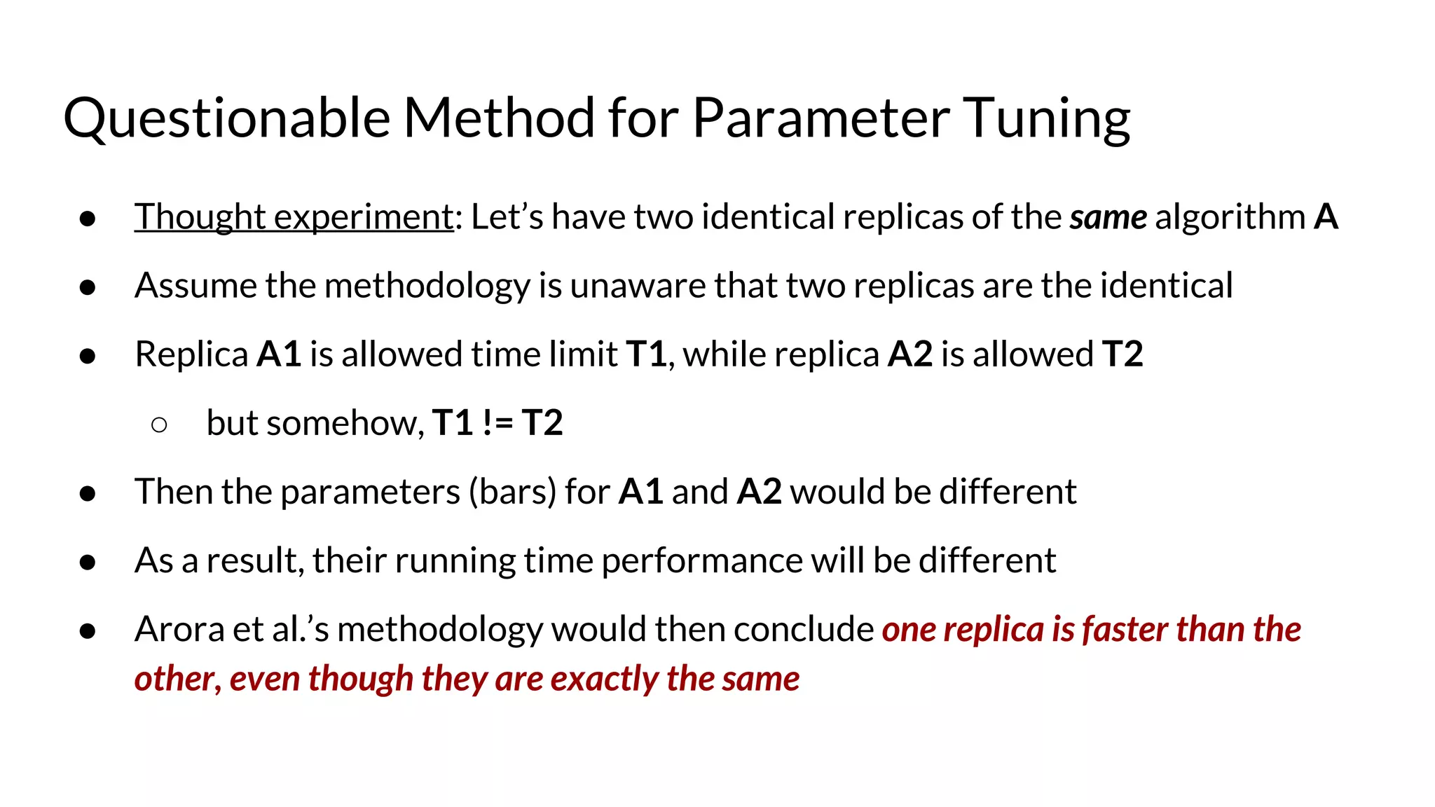
● Arora et al.’s design question: “How long does it take for each algorithm to
reach its ‘near-optimal’ empirical accuracy”
● Their experimental design/methodology is:
○ For each influence maximization Algorithm-A,
○ Identify a parameter p that controls the trade-off between running time and spread
achieved.
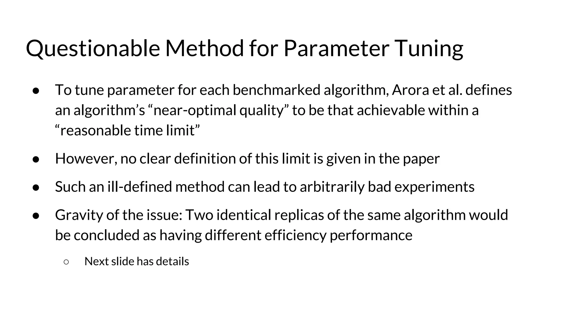
○ Choose value p* for the parameter, such that in a given “reasonable time limit” T (not
defined in [1]), Algorithm-A can achieve its best spread.
○ Compare all algorithms’ running time at their each individual p*.
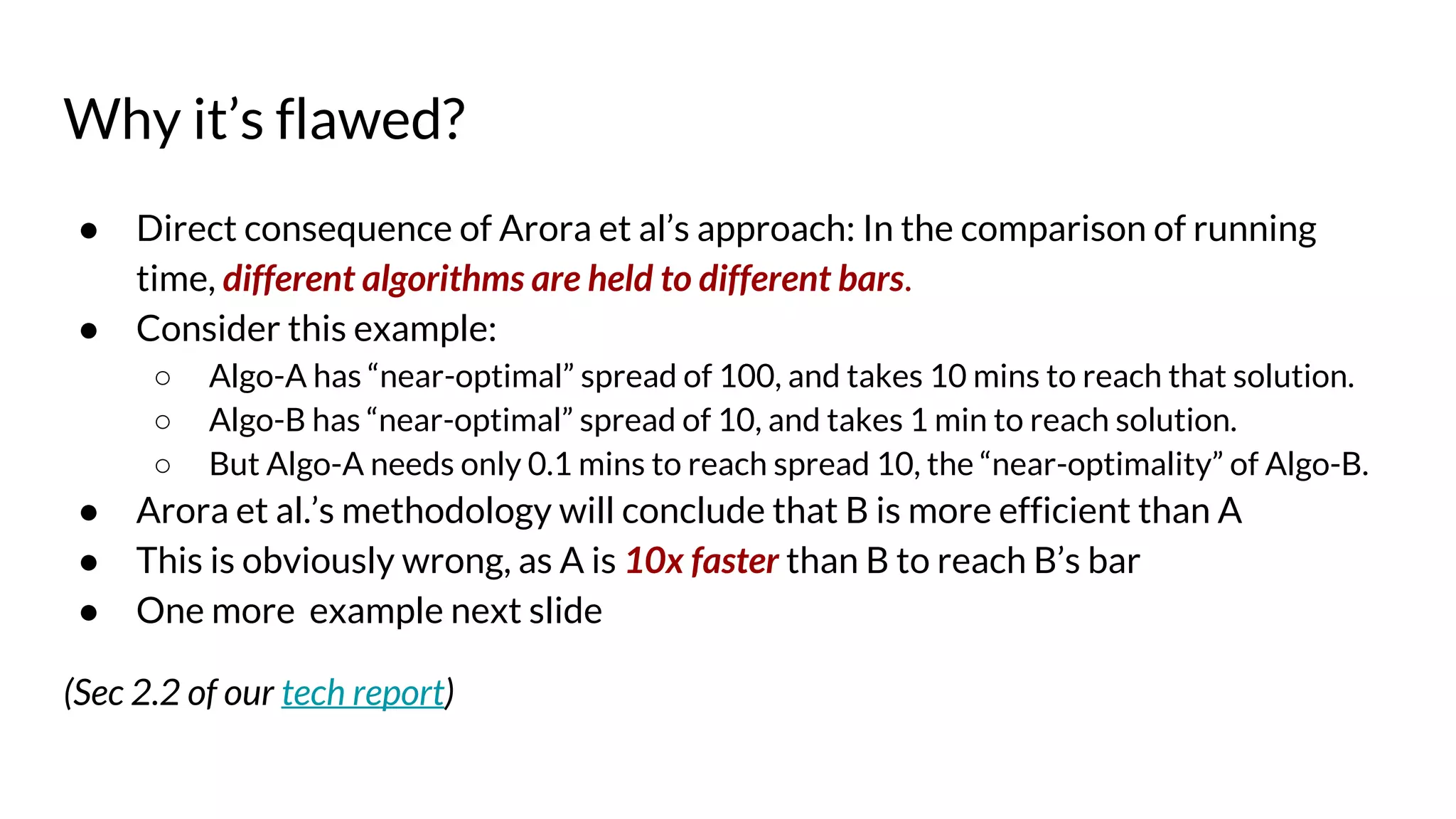
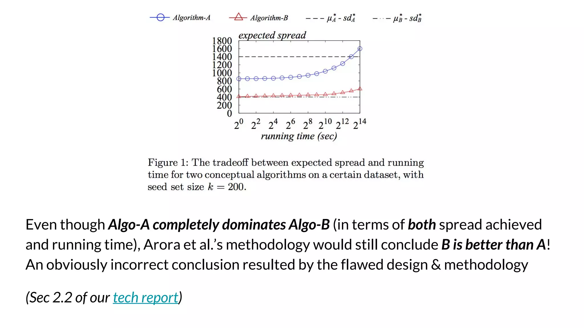
● This is a flawed methodology that will lead to scientifically incorrect results (see
next few slides)
(Sec 2.2 of our tech report)

7. Why it’s flawed?
● Direct consequence of Arora et al’s approach: In the comparison of running
time, different algorithms are held to different bars.
● Consider this example:
○ Algo-A has “near-optimal” spread of 100, and takes 10 mins to reach that solution.
○ Algo-B has “near-optimal” spread of 10, and takes 1 min to reach solution.
○ But Algo-A needs only 0.1 mins to reach spread 10, the “near-optimality” of Algo-B.
● Arora et al.’s methodology will conclude that B is more efficient than A
● This is obviously wrong, as A is 10x faster than B to reach B’s bar
● One more example next slide
(Sec 2.2 of our tech report)

8. Even though Algo-A completely dominates Algo-B (in terms of both spread achieved
and running time), Arora et al.’s methodology would still conclude B is better than A!
An obviously incorrect conclusion resulted by the flawed design & methodology
(Sec 2.2 of our tech report)

9. Unreproducible Results for Parameter Selection
● We are unable to reproduce Figure 12 in Arora et al, which are experiments for
determining the optimal parameter p* for each algorithm
● In a nutshell, Figure 12 presented standard deviations values with 10K samples
in each setting (per algo/model/dataset combo)
● We obtained standard deviations values are 10 times larger than Arora et al.’s
○ Validated with both UBC and NTU servers
● Impact: Incorrect Figure 12 results → all benchmarking experiments can be
wrong & need to be re-run, as the parameter setup are erroneous in the first
place
(See Sec 2.3 of our tech report for details on why discrepancies occurred)

10. Questionable Method for Parameter Tuning
● To tune parameter for each benchmarked algorithm, Arora et al. defines
an algorithm’s “near-optimal quality” to be that achievable within a
“reasonable time limit”
● However, no clear definition of this limit is given in the paper
● Such an ill-defined method can lead to arbitrarily bad experiments
● Gravity of the issue: Two identical replicas of the same algorithm would
be concluded as having different efficiency performance
○ Next slide has details

11. Questionable Method for Parameter Tuning
● Thought experiment: Let’s have two identical replicas of the same algorithm A
● Assume the methodology is unaware that two replicas are the identical
● Replica A1 is allowed time limit T1, while replica A2 is allowed T2
○ but somehow, T1 != T2
● Then the parameters (bars) for A1 and A2 would be different
● As a result, their running time performance will be different
● Arora et al.’s methodology would then conclude one replica is faster than the
other, even though they are exactly the same

12. Misclaims related to IMM algorithm [3]
and TIM+ algorithm [2]

13. TIM+ and IMM algorithms
● Both are fast and highly scalable (1-1/e-epsilon)-approximation algorithms
○ Underlying methodology: Sampling reverse-reachable set for seed selection
● IMM improves upon TIM+ by using martingale theory to draw much fewer
samples, for any given epsilon (i.e., same worst-case performance guarantee)
● Both papers [2][3] showed that very small epsilon (< 0.1) increases running time
a lot but does not further improve quality too much (i.e., the trade-off at that
point isn’t worth it)

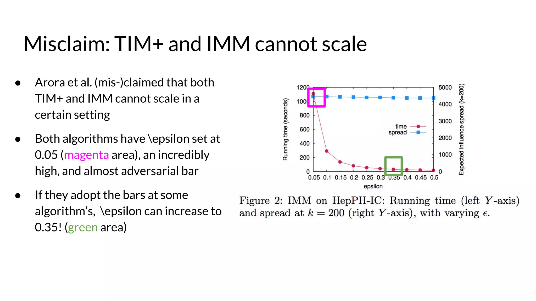
14. ● Running time (left Y-axis) sharply
decreases as epsilon goes up.
● Solution quality (right Y-axis) is
only marginally affected.
● E.g., epsilon at 0.05 vs. 0.5, the
running time difference is 68x, but
accuracy difference is only 2.1%.
● Quite similar trend for TIM+
● See original papers [2][3] for
details.
Efficiency & quality tradeoff for IMM

15. Misclaim: TIM+ and IMM cannot scale
● Arora et al. (mis-)claimed that both
TIM+ and IMM cannot scale in a
certain setting
● Both algorithms have epsilon set at
0.05 (magenta area), an incredibly
high, and almost adversarial bar
● If they adopt the bars at some
algorithm’s, epsilon can increase to
0.35! (green area)

16. Misclaim: TIM+ is better than IMM on LT model
● Arora et al. ignored theoretical guarantees but opted for empirical accuracies,
yet again with different bars of accuracy.
● For LT model, they set the bar of IMM (epsilon = 0.05) much higher than TIM+
(epsilon = 0.1)
○ See previous slide for illustration
● Erroneously conclude IMM is not as scalable as TIM+
● Analogy of their error: Chebyshev’s inequality is empirically more efficient than
Chernoff bound!
(See Sec 3.1 of our tech report on the Chernoff vs. Chebyshev example)

17. Misclaims related to SimPath [4]

18. Mis-claims based on infinite loops
● Arora et al [1] stated that the SimPath algorithm [4] fails to finish on two
datasets after 2400 hours (100 days), using code released by authors of [4].
● Our attempts to reproduce found that SimPath finishes within 8.6 and 667
minutes respectively on those two datasets (UBC server)
○ 8.6 minutes = 0.006% of 2400 hours
○ 667 minutes = 0.463% of 2400 hours
● Reasons for discrepancies: Arora et al. [1] failed to preprocess datasets
correctly as per the source code released by [4], and ran into infinite loops and
got stuck for 100 days
(Sec 3.2 of our tech report)

19. More mis-claims on SimPath
● Misclaim: LDAG [5] is better than SimPath on “LT-uniform” model
● Refutation: The two datasets where Arora et al. stuck in infinite loops happen
to be prepared according to “LT-uniform” model. This is a corollary of the
previous misclaim
● Misclaim: LDAG is overall better than SimPath
● Refutation: This is a blanket statement contradicting experimental results:

20. Other Misclaims

21. “EaSyIM [6] is one of the best IM algorithm”
● Arora et al. recommends that EaSyIM heuristic [6] as one of the best IM
algorithms, comparable to IMM and TIM+
○ EaSyIM [6] and this SIGMOD paper [1] share two co-authors: Arora, Galhotra
● However, their own Table 3 (see below) illustrates EaSyIM is not scalable at all,
providing a refutation to this misleading claim
○ In both WC and LT settings, EaSyIM failed to finish on 3 largest datasets after 40 hours, while
IMM and TIM finished on all datasets. In IC setting, it failed on 2 largest datasets

22. “EaSyIM is Most Memory-Efficient”
● Misclaim: EaSyIM [6] is the “most-memory efficient” algorithm
● Their justification: EaSyIM only stores a scalar-value per each node in graph
● Refutation: A meaningless statement that ignores the trade-off between
memory consumption and quality of solution:
○ E.g., many more advanced algorithms such as IMM [3] and TIM+ [2] utilizes more
memory to achieve better solutions
○ The same “one scalar per node” argument can be used for arguing that a naive algorithm that
randomly select k seeds is the most memory efficient, but is this useful at all?

23. Conclusions and Key Takeaways
● Our technical report critically reviews the SIGMOD benchmarking paper by
Arora et al. [1], claiming to debunk “myths” of influence maximization research
● We found that Arora et al. [1] is riddled with problematic issues, including:
○ ill-designed and flawed experimental methodology
○ unreproducible results in critical experiments
○ more than 10 mis-claims on a variety of previously published algorithms
○ misleading conclusions in support of an unscalable heuristic (EaSyIM)

24. References
[1]. A. Arora, S. Galhotra, and S. Ranu. Debunking the myths of influence maximization: An in-depth
benchmarking study. In SIGMOD 2017.
[2]. Y. Tang, X. Xiao, and Y. Shi. Influence maximization: near-optimal time complexity meets practical
efficiency. In SIGMOD, pages 75–86, 2014.
[3]. Y. Tang, Y. Shi, and X. Xiao. Influence maximization in near-linear time: a martingale approach. In
SIGMOD, pages 1539–1554, 2015.
[4]. A. Goyal, W. Lu, and L. V. S. Lakshmanan. SimPath: An efficient algorithm for influence maximization
under the linear threshold model. In ICDM, pages 211–220, 2011.
[5]. W. Chen, Y. Yuan, and L. Zhang. Scalable influence maximization in social networks under the linear
threshold model. In ICDM, pages 88–97, 2010.
[6]. S. Galhotra, A. Arora, and S. Roy. Holistic influence maximization: Combining scalability and efficiency
with opinion-aware models. In SIGMOD, pages 743–758, 2016.

25. For more details of all refutations, please check out:
https://arxiv.org/abs/1705.05144