SlideShare a Scribd company logo
1 of 37
Download to read offline
Chapter 4. Neural Networks Based on
Competition
• Competition is important for NN
– Competition between neurons has been observed in
biological nerve systems
– Competition is important in solving many problems
To classify an input pattern
into one of the m classes
– idea case: one class node
has output 1, all other 0 ;
– often more than one class
nodes have non-zero output
– If these class nodes compete with each other, maybe only
one will win eventually (winner-takes-all). The winner
represents the computed classification of the input
C_m
C_1
x_n
x_1
INPUT CLASSIFICATION
• Winner-takes-all (WTA):
– Among all competing nodes, only one will win and all
others will lose
– We mainly deal with single winner WTA, but multiple
winners WTA are possible (and useful in some
applications)
– Easiest way to realize WTA: have an external, central
arbitrator (a program) to decide the winner by
comparing the current outputs of the competitors (break
the tie arbitrarily)
– This is biologically unsound (no such external arbitrator
exists in biological nerve system).
• Ways to realize competition in NN
– Lateral inhibition (Maxnet, Mexican hat)
output of each node feeds
to others through inhibitory
connections (with negative weights)
– Resource competition
• output of x_k is distributed to
y_i and y_j proportional to w_ki
and w_kj, as well as y_i and y_j
• self decay
• biologically sound
• Learning methods in competitive networks
– Competitive learning
– Kohonen learning (self-organizing map, SOM)
– Counter-propagation net
– Adaptive resonance theory (ART) in Ch. 5
y_j
y_i
0
<
ij
w
y_i y_j
x_k
kj
w
ki
w
0
<
ii
w 0
<
jj
w
Fixed-weight Competitive Nets
• Notes:
– Competition:
• iterative process until the net stabilizes (at most one node
with positive activation)
– where m is the # of competitors
• too small: takes too long to converge
• too big: may suppress the entire network (no winner)
• Maxnet
– Lateral inhibition between
competitors


 >
=



−
=
=
otherwise
0
0
if
)
(
:
function
activation
otherwise
if
1
:
weights
x
x
x
f
j
i
wij
ε
ε
,
/
1
0 m
<
< ε
ε
ε
ε
ε
ε
Mexical Hat
• Architecture: For a given node,
– close neighbors: cooperative (mutually excitatory , w > 0)
– farther away neighbors: competitive (mutually
inhibitory,w < 0)
– too far away neighbors: irrelevant (w = 0)
• Need a definition of distance (neighborhood):
– one dimensional: ordering by index (1,2,…n)
– two dimensional: lattice





>
=
<
=
k
j
i
k
j
i
c
k
j
i
c
wij
)
,
(
distance
if
0
)
,
(
distance
if
)
,
(
distance
if
weights
2
1
:
function
ramp
max
max
max
0
0
0
)
(
function
activation





>
≤
≤
<
=
x
if
x
if
x
x
if
x
f
• Equilibrium:
– negative input = positive input for all nodes
– winner has the highest activation;
– its cooperative neighbors also have positive activation;
– its competitive neighbors have negative activations.
)
0
.
0
,
39
.
0
,
14
.
1
,
66
.
1
,
14
.
1
,
39
.
0
,
0
.
0
(
)
2
(
)
9
.
0
,
38
.
0
,
06
.
1
,
16
.
1
,
06
.
1
,
38
.
0
,
0
.
0
(
)
1
(
)
0
.
0
,
5
.
0
,
8
.
0
,
0
.
1
,
8
.
0
,
5
.
0
,
0
.
0
(
)
0
(
:
example
=
=
=
x
x
x
Hamming Network
• Hamming distance of two vectors, of
dimension n,
– Number of bits in disagreement.
– In bipolar:
y
x and
distance
Hamming
shorter
larger
larger
)
(
5
.
0
2
distance
hamming
and
in
different
bits
of
number
is
and
in
agreement
in
bits
of
number
is
:
where
⇒
⇒
⋅
+
⋅
=
−
=
⋅
−
=
−
=
⋅
a
y
x
n
y
x
a
n
a
y
x
a
n
d
y
x
d
y
x
a
d
a
y
x
• Suppose a space of patterns is divided into k classes, each
class has an exampler (representative) vector .
• An input belongs to class i, if and only if is closer to
than to any other , i.e.,
• Hamming net is such a classifier:
– Weights: let represent class j
– The total input to
j
e
x x
i
j
e
x
e
x j
i ≠
∀
⋅
≥
⋅
i
e j
e
j
Y
n
b
e
w j
j
j 5
.
0
,
5
.
0 =
=
•
j
j
i
i
ij
j
j
a
n
e
x
x
w
b
in
y
=
+
⋅
=
+
= ∑
)
(
2
1
_
j
Y
• Upper layer: MAX net
– it takes the y_in as its initial value, then iterates toward
stable state
– one output node with highest y_in will be the winner
because its weight vector is closest to the input vector
• As associative memory:
– each corresponds to a stored pattern;
– pattern connection/completion;
– storage capacity
total # of nodes: k
total # of patterns stored: k
capacity: k (or k/k = 1)
j
Y
• Implicit lateral inhibition by competing limited
resources: the activation of the input nodes
y_1 y_j y_m
x_i i
ij
j
j
j
i
ij
ij
i
ij
j
x
w
y
y
y
x
w
in
y
in
y
in
y
of
share
larger
takes
larger
)
(
_
_
_
α
α
β
β −
⋅
=
= ∑
decay
W_ij
Competitive Learning
• Unsupervised learning
• Goal:
– Learn to form classes/clusters of examplers/sample patterns
according to similarities of these exampers.
– Patterns in a cluster would have similar features
– No prior knowledge as what features are important for
classification, and how many classes are there.
• Architecture:
– Output nodes:
Y_1,…….Y_m,
representing the m classes
– They are competitors
(WTA realized either by
an external procedure or
by lateral inhibition as in Maxnet)
• Training:
– Train the network such that the weight vector w.j associated
with Y_j becomes the representative vector of the class of
input patterns Y_j is to represent.
– Two phase unsupervised learning
• competing phase:
– apply an input vector randomly chosen from sample set.
– compute output for all y:
– determine the winner (winner is not given in training
samples so this is unsupervised)
• rewarding phase:
– the winner is reworded by updating its weights (weights
associated with all other output nodes are not updated)
• repeat the two phases many times (and gradually reduce
the learning rate) until all weights are stabilized.
x
j
j w
x
y •
⋅
=
x
• Weight update:
– Method 1: Method 2
In each method, is moved closer to x
– Normalizing the weight vector to unit length after it is
updated
)
( j
j
w
x
w •
• −
=
∆ α
α x
w j
α
α
=
∆ •
j
j
j w
w
w •
•
• ∆
+
=
j
j
j
w
w
w
•
•
• =
w_j
x
x-w_j
a(x-w_j)
w_j +a(x-w_j)
j
w•
w_j
x+w_j
w_j+ ax
ax
• is moving to the center of a cluster of sample vectors after
repeated weight updates
– Three examplers:
S(1), S(2) and S(3)
– Initial weight vector w_j(0)
– After successively trained
by S(1), S(2), and S(3),
the weight vector
changes to w_j(1),
w_j(2), and w_j(3)
j
w•
S(2)
S(1)
S(3)
w_j(0)
w_j(1)
w_j(2)
w_j(3)
Examples
• A simple example of competitive learning (pp. 172-175)
– 4 vectors of dimension 4 in 2 classes (4 input nodes, 2 output nodes)
S(1) = (1, 1, 0, 0) S(2) = (0, 0, 0, 1)
S(3) = (1, 0, 0, 0) S(4) = (0, 0, 1, 1)
– Initialization: , weight matrix:
– Training with S(1)
6
.
0
=
α
α












=
3
.
9
.
7
.
5
.
4
.
6
.
8
.
2
.
W
86
.
1
)
0
9
(.
)
0
5
(.
)
1
6
(.
)
1
2
(.
)
1
(
)
1
(
2
2
2
2
1
=
−
+
−
+
−
+
−
=
−
= •
w
S
D
wins
2
class
,
98
.
0
)
1
(
)
1
( 2 =
−
= •
w
S
D












=












−












+












=
•
12
.
28
.
76
.
92
.
)
3
.
7
.
4
.
8
.
0
0
1
1
(
6
.
0
3
.
7
.
4
.
8
.
2
w












=
12
.
9
.
28
.
5
.
76
.
6
.
92
.
2
.
then W
– Similarly, after training with
S(2) = (0, 0, 0, 1) ,
in which class 1 wins,
weight matrix becomes
– At the end of the first iteration
(each of the 4 vectors are used),
weight matrix becomes
– Reduce
– Repeat training. After 10
iterations, weight matrix becomes
3
.
0
6
.
0
5
.
0
5
.
0 =
⋅
=
⋅
= α
α
α
α












=
12
.
96
.
28
.
20
.
76
.
24
.
92
.
08
.
W












=
048
.
980
.
110
.
680
.
300
.
096
.
970
.
032
.
W
α
α












→












−
−
−
−
=
0
.
0
0
.
1
0
.
0
5
.
0
5
.
0
0
.
0
0
.
1
0
.
0
16
0
.
1
000000
.
1
16
3
.
2
5100000
.
4900000
.
16
0
.
2
000000
.
1
17
7
.
6
e
e
e
e
W
• S(1) and S(3) belong
to class 2
• S(2) and S(4) belong
to class 1
• w_1 and w_2 are the
centroids of the two
classes
Comments
1. Ideally, when learning stops, each is close to the
centroid of a group/cluster of sample input vectors.
2. To stabilize , the learning rate may be reduced slowly
toward zero during learning.
3. # of output nodes:
– too few: several clusters may be combined into one class
– too many: over classification
– ART model (later) allows dynamic add/remove output nodes
4. Initial :
– training samples known to be in distinct classes, provided
such info is available
– random (bad choices may cause anomaly)
j
w•
j
w• α
α
j
w•
Example
will always win no matter
the sample is from which class
is stuck and will not participate
in learning
unstuck:
let output nodes have some conscience
temporarily shot off nodes which have had very high
winning rate (hard to determine what rate should be
considered as “very high”)
2
•
w
1
•
w
w_1
w_2
Kohonen Self-Organizing Maps (SOM)
• Competitive learning (Kohonen 1982) is a special case of
SOM (Kohonen 1989)
• In competitive learning,
– the network is trained to organize input vector space into
subspaces/classes/clusters
– each output node corresponds to one class
– the output nodes are not ordered: random map
w_3
w_2
cluster_1
cluster_3
cluster_2
w_1
• The topological order of the
three clusters is 1, 2, 3
• The order of their maps at
output nodes are 2, 3, 1
• The map does not preserve
the topological order of the
training vectors
• Topographic map
– a mapping that preserves neighborhood relations
between input vectors, (topology preserving or feature
preserving).
– if are two neighboring input vectors ( by
some distance metrics),
– their corresponding winning output nodes (classes), i
and j must also be close to each other in some fashion
– one dimensional: line or ring, node i has neighbors
or
– two dimensional:grid.
rectangular: node(i, j) has neighbors:
hexagonal: 6 neighbors
2
and
1 x
x
1
±
i
))
1
,
1
(
additional
or
(
),
,
1
(
),
1
,
( ±
±
±
± j
i
j
i
j
i
n
i mod
1
±
• Biological motivation
– Mapping two dimensional continuous inputs from
sensory organ (eyes, ears, skin, etc) to two dimensional
discrete outputs in the nerve system.
• Retinotopic map: from eye (retina) to the visual cortex.
• Tonotopic map: from the ear to the auditory cortex
– These maps preserve topographic orders of input.
– Biological evidence shows that the connections in these
maps are not entirely “pre-programmed” or “pre-wired”
at birth. Learning must occur after the birth to create
the necessary connections for appropriate topographic
mapping.
SOM Architecture
• Two layer network:
– Output layer:
• Each node represents a class (of inputs)
•
• Neighborhood relation is defined over these nodes
Each node cooperates with all its neighbors within
distance R and competes with all other output nodes.
• Cooperation and competition of these nodes can be
realized by Mexican Hat model
R = 0: all nodes are competitors (no cooperative)
à random map
R > 0: à topology preserving map
∑
=
⋅
= •
i
i
ij
j
j x
w
w
x
y
:
activation
Node
SOM Learning
1. Initialize , and to a small value
2. For a randomly selected input sample/exampler
determine the winning output node J
either is maximum or
is minimum
3. For all output node j with , update the weight
4. Periodically reduce and R slowly.
5. Repeat 2 - 4 until the network stabilized.
x
J
W
x •
⋅
∑ −
=
− •
i
i
ij
J x
w
w
x 2
)
(
R
j
J ≤
−
)
( ij
ij
ij w
x
w
w −
+
= α
α
α
α
nodes
output
all
for
j
W• α
α
Notes
1. Initial weights: small random value from (-e, e)
2. Reduction of :
Linear:
Geometric:
may be 1 or greater than 1
3. Reduction of R:
should be much slower than reduction.
R can be a constant through out the learning.
4. Effect of learning
For each input x, not only the weight vector of winner J
is pulled closer to x, but also the weights of J’s close
neighbors (within the radius of R).
5. Eventually, becomes close (similar) to . The
classes they represent are also similar.
6. May need large initial R
α
α
α
α
α
α
α
α ∆
−
=
∆
+ )
(
)
( t
t
t
β
β
α
α
α
α )
(
)
( t
t
t =
∆
+
t
∆
0
)
(
while
1
)
(
)
( >
−
=
∆
+ t
R
t
R
t
t
R
α
α
j
w• 1
±
• j
w
Examples
• A simple example of competitive learning (pp. 172-175)
– 4 vectors of dimension 4 in 2 classes (4 input nodes, 2 output nodes)
S(1) = (1, 1, 0, 0) S(2) = (0, 0, 0, 1)
S(3) = (1, 0, 0, 0) S(4) = (0, 0, 1, 1)
– Initialization: , weight matrix:
– Training with S(1)
6
.
0
=
α
α












=
3
.
9
.
7
.
5
.
4
.
6
.
8
.
2
.
W
86
.
1
)
0
9
(.
)
0
5
(.
)
1
6
(.
)
1
2
(.
)
1
(
)
1
(
2
2
2
2
1
=
−
+
−
+
−
+
−
=
−
= •
w
S
D
wins
2
class
,
98
.
0
)
1
(
)
1
( 2 =
−
= •
w
S
D












=












−












+












=
•
12
.
28
.
76
.
92
.
)
3
.
7
.
4
.
8
.
0
0
1
1
(
6
.
0
3
.
7
.
4
.
8
.
2
w












=
12
.
9
.
28
.
5
.
76
.
6
.
92
.
2
.
then W
• How to illustrate Kohonen map
– Input vector: 2 dimensional
Output vector: 1 dimensional line/ring or 2 dimensional grid.
Weight vector is also 2 dimension
– Represent the topology of output nodes by points on a 2 dimensional
plane. Plotting each output node on the plane with its weight vector
as its coordinates.
– Connecting neighboring output nodes by a line
output nodes: (1, 1) (2, 1) (1, 2)
weight vectors: (0.5, 0.5) (0.7, 0.2) (0.9, 0.9)
C(1, 2)
C(2, 1)
C(1, 1)
Traveling Salesman Problem (TSP) by SOM
• Each city is represented as a 2 dimensional input vector (its
coordinates (x, y)),
• Output nodes C_j form a one dimensional SOM, each node
corresponds to a city.
• Initially, C_1, ... , C_n have random weight vectors
• During learning, a winner C_j on an input (x, y) of city I, not only
moves its w_j toward (x, y), but also that of of its neighbors
(w_(j+1), w_(j-1)).
• As the result, C_(j-1) and C_(j+1) will later be more likely to win
with input vectors similar to (x, y), i.e, those cities closer to I
• At the end, if a node j represents city I, it would end up to have its
neighbors j+1 or j-1 to represent cities similar to city I (i,e., cities
close to city I).
• This can be viewed as a concurrent greedy algorithm
Initial position
Two candidate solutions:
ADFGHIJBC
ADFGHIJCB
Additional examples
Counter propagation network (CPN)
• Basic idea of CPN
– Purpose: fast and coarse approximation of vector mapping
• not to map any given x to its with given precision,
• input vectors x are divided into clusters/classes.
• each cluster of x has one output y, which is (hopefully) the
average of for all x in that class.
– Architecture: Simple case: FORWARD ONLY CPN,
)
(x
y φ
φ
=
)
(x
φ
φ
)
(x
φ
φ
m
p
n
k
j
j
j
i
y
z
x
y
w
z
v
x
y
z
x 1
1
1
•
•
from (input)
features to class
from class to
(output) features
– Learning in two phases:
– training sample x:y where is the precise mapping
– Phase1: is trained by competitive learning to become the
representative vector of a cluster of input vectors x (use sample x
only)
1. For a chosen x, feedforward to determined the winning
2.
3. Reduce , then repeat steps 1 and 2 until stop condition is met
– Phase 2: is trained by delta rule to be an average output of
where x is an input vector that causes to win (use both x and y).
1. For a chosen x, feedforward to determined the winning
2. (optional)
3.
4. Repeat steps 1 – 3 until stop condition is met
)
(x
y φ
φ
=
j
v•
•
j
w )
(x
φ
φ
j
z
j
z
))
(
(
)
(
)
( old
v
x
old
v
new
v ij
i
ij
ij −
+
= α
α
α
α
))
(
(
)
(
)
( old
v
x
old
v
new
v ij
i
ij
ij −
+
= α
α
))
(
(
)
(
)
( old
w
y
old
w
new
w jk
k
jk
jk −
+
= α
α
j
z
• A combination of both unsupervised learning (for in phase 1) and
supervised learning (for in phase 2).
• After phase 1, clusters are formed among sample input x , each is
a representative of a cluster (average).
• After phase 2, each cluster j maps to an output vector y, which is the
average of
• View phase 2 learning as following delta rule
•
Notes
j
v•
•
j
w
j
v•
{ }
:
)
( j
cluster
x
x ∈
φ
φ
wins
when
)
(
2
)
(
because
,
where
)
(
2
j
j
jk
k
j
jk
k
jk
jk
jk
jk
k
jk
k
jk
jk
z
z
w
y
z
w
y
w
w
E
w
E
w
y
w
y
w
w
−
−
=
−
∂
∂
=
∂
∂
∂
∂
−
∝
−
−
+
=
∑
α
α
win
make
that
samples
training
all
of
mean
the
is
where
)
(
)
(
and
)
(
,
when
,
shown that
be
can
It
x
x
x
t
w
x
t
v
t
j
j φ
φ
→
→
∞
→
•
•
)
1
(
)
(
)
1
(
)
1
(
as
rewriteen
be
can
rule
update
Weight
similar.)
is
of
(proof
on
only
Show
+
+
−
=
+ t
x
t
v
t
v
w
v
i
ij
ij
jk
ij
α
α
α
α
[ ]
t
i
i
i
i
i
i
ij
i
i
ij
i
ij
ij
x
t
x
t
x
t
x
t
x
t
x
t
v
t
x
t
x
t
v
t
x
t
v
t
v
)
1
)(
1
(
...
)
1
)(
1
(
)
1
)(
(
)
1
(
)
1
(
)
(
)
1
(
)
1
(
)
1
(
)
1
(
))
(
)
1
(
)
1
)((
1
(
)
1
(
)
(
)
1
(
)
1
(
2
2
α
α
α
α
α
α
α
α
α
α
α
α
α
α
α
α
α
α
α
α
α
α
α
α
α
α
α
α
−
+
−
−
+
−
+
+
≈
+
+
−
+
−
−
=
+
+
+
−
−
−
=
+
+
−
=
+
x
x
x
x
E
t
x
E
t
x
E
x
t
x
t
x
E
t
v
E
t
i
t
t
i
i
ij
=
−
−
⇒
−
+
−
+
=
−
+
−
+
+
=
−
+
−
+
+
=
+
)
1
(
1
1
]
)
1
....(
)
1
(
1
[
))]
1
(
(
)
1
...(
))
(
(
)
1
(
))
1
(
(
[
]
)
1
(
...
)
1
)(
(
)
1
(
(
[
)]
1
(
[ 1
α
α
α
α
α
α
α
α
α
α
α
α
α
α
α
α
α
α
α
α
α
α
then
set,
training
the
from
randomly
drawn
are
If x
• After training, the network works like a look-up of math
table.
– For any input x, find a region where x falls (represented by
the wining z node);
– use the region as the index to look-up the table for the
function value.
– CPN works in multi-dimensional input space
– More cluster nodes (z), more accurate mapping.
• If both
we can establish bi-directional approximation
• Two pairs of weights matrices:
V ( ) and U ( ) for approx. map x to
W ( ) and T ( ) for approx. map y to
• When x:y is applied ( ), they can
jointly determine the winner J or separately for
• pp. 196 –206 for more details
exist
)
(
function
inverse
its
and
)
( 1
y
x
x
y −
=
= φ
φ
φ
φ
z
x to )
(x
y φ
φ
=
)
(
* x
x φ
φ
=
Y
y
X
x on
and
on
Jy
Jx z
z ,
Full CPN
y
z to
z
y to x
z to

More Related Content

What's hot

Artificial Neural Networks Lect2: Neurobiology & Architectures of ANNS
Artificial Neural Networks Lect2: Neurobiology & Architectures of ANNSArtificial Neural Networks Lect2: Neurobiology & Architectures of ANNS
Artificial Neural Networks Lect2: Neurobiology & Architectures of ANNSMohammed Bennamoun
 
Neural network
Neural networkNeural network
Neural networkSilicon
 
Animation as-the-final-step-in-the-dynamics-experience
Animation as-the-final-step-in-the-dynamics-experienceAnimation as-the-final-step-in-the-dynamics-experience
Animation as-the-final-step-in-the-dynamics-experienceVíctor Quezada
 
Artificial Neural Network
Artificial Neural NetworkArtificial Neural Network
Artificial Neural NetworkPratik Aggarwal
 
Artificial Neural Network
Artificial Neural NetworkArtificial Neural Network
Artificial Neural NetworkAtul Krishna
 
Nearest Class Mean Metric Learning
Nearest Class Mean Metric LearningNearest Class Mean Metric Learning
Nearest Class Mean Metric LearningSangjun Han
 
Dr. kiani artificial neural network lecture 1
Dr. kiani artificial neural network lecture 1Dr. kiani artificial neural network lecture 1
Dr. kiani artificial neural network lecture 1Parinaz Faraji
 
Introduction to Deep Neural Network
Introduction to Deep Neural NetworkIntroduction to Deep Neural Network
Introduction to Deep Neural NetworkLiwei Ren任力偉
 
Adaline madaline
Adaline madalineAdaline madaline
Adaline madalineNagarajan
 
Fem in geotech engineering
Fem in geotech engineeringFem in geotech engineering
Fem in geotech engineeringJEET TRIVEDI
 
Finite element method (matlab) milan kumar rai
Finite element method (matlab) milan kumar raiFinite element method (matlab) milan kumar rai
Finite element method (matlab) milan kumar raiMilan Kumar Rai
 
Finite elements for 2‐d problems
Finite elements  for 2‐d problemsFinite elements  for 2‐d problems
Finite elements for 2‐d problemsTarun Gehlot
 
Basic Learning Algorithms of ANN
Basic Learning Algorithms of ANNBasic Learning Algorithms of ANN
Basic Learning Algorithms of ANNwaseem khan
 
Loss functions (DLAI D4L2 2017 UPC Deep Learning for Artificial Intelligence)
Loss functions (DLAI D4L2 2017 UPC Deep Learning for Artificial Intelligence)Loss functions (DLAI D4L2 2017 UPC Deep Learning for Artificial Intelligence)
Loss functions (DLAI D4L2 2017 UPC Deep Learning for Artificial Intelligence)Universitat Politècnica de Catalunya
 
Neural Network Fundamentals
Neural Network FundamentalsNeural Network Fundamentals
Neural Network FundamentalsManoj Kumar
 
(Artificial) Neural Network
(Artificial) Neural Network(Artificial) Neural Network
(Artificial) Neural NetworkPutri Wikie
 
Aplicaciones de espacios y subespacios vectoriales en la carrera de tecnologi...
Aplicaciones de espacios y subespacios vectoriales en la carrera de tecnologi...Aplicaciones de espacios y subespacios vectoriales en la carrera de tecnologi...
Aplicaciones de espacios y subespacios vectoriales en la carrera de tecnologi...ERIKAMARIAGUDIOSANTA
 
Neural network 20161210_jintaekseo
Neural network 20161210_jintaekseoNeural network 20161210_jintaekseo
Neural network 20161210_jintaekseoJinTaek Seo
 

What's hot (20)

Artificial Neural Networks Lect2: Neurobiology & Architectures of ANNS
Artificial Neural Networks Lect2: Neurobiology & Architectures of ANNSArtificial Neural Networks Lect2: Neurobiology & Architectures of ANNS
Artificial Neural Networks Lect2: Neurobiology & Architectures of ANNS
 
Neural network
Neural networkNeural network
Neural network
 
Animation as-the-final-step-in-the-dynamics-experience
Animation as-the-final-step-in-the-dynamics-experienceAnimation as-the-final-step-in-the-dynamics-experience
Animation as-the-final-step-in-the-dynamics-experience
 
Artificial Neuron network
Artificial Neuron network Artificial Neuron network
Artificial Neuron network
 
Artificial Neural Network
Artificial Neural NetworkArtificial Neural Network
Artificial Neural Network
 
Artificial Neural Network
Artificial Neural NetworkArtificial Neural Network
Artificial Neural Network
 
Nearest Class Mean Metric Learning
Nearest Class Mean Metric LearningNearest Class Mean Metric Learning
Nearest Class Mean Metric Learning
 
Neural network
Neural networkNeural network
Neural network
 
Dr. kiani artificial neural network lecture 1
Dr. kiani artificial neural network lecture 1Dr. kiani artificial neural network lecture 1
Dr. kiani artificial neural network lecture 1
 
Introduction to Deep Neural Network
Introduction to Deep Neural NetworkIntroduction to Deep Neural Network
Introduction to Deep Neural Network
 
Adaline madaline
Adaline madalineAdaline madaline
Adaline madaline
 
Fem in geotech engineering
Fem in geotech engineeringFem in geotech engineering
Fem in geotech engineering
 
Finite element method (matlab) milan kumar rai
Finite element method (matlab) milan kumar raiFinite element method (matlab) milan kumar rai
Finite element method (matlab) milan kumar rai
 
Finite elements for 2‐d problems
Finite elements  for 2‐d problemsFinite elements  for 2‐d problems
Finite elements for 2‐d problems
 
Basic Learning Algorithms of ANN
Basic Learning Algorithms of ANNBasic Learning Algorithms of ANN
Basic Learning Algorithms of ANN
 
Loss functions (DLAI D4L2 2017 UPC Deep Learning for Artificial Intelligence)
Loss functions (DLAI D4L2 2017 UPC Deep Learning for Artificial Intelligence)Loss functions (DLAI D4L2 2017 UPC Deep Learning for Artificial Intelligence)
Loss functions (DLAI D4L2 2017 UPC Deep Learning for Artificial Intelligence)
 
Neural Network Fundamentals
Neural Network FundamentalsNeural Network Fundamentals
Neural Network Fundamentals
 
(Artificial) Neural Network
(Artificial) Neural Network(Artificial) Neural Network
(Artificial) Neural Network
 
Aplicaciones de espacios y subespacios vectoriales en la carrera de tecnologi...
Aplicaciones de espacios y subespacios vectoriales en la carrera de tecnologi...Aplicaciones de espacios y subespacios vectoriales en la carrera de tecnologi...
Aplicaciones de espacios y subespacios vectoriales en la carrera de tecnologi...
 
Neural network 20161210_jintaekseo
Neural network 20161210_jintaekseoNeural network 20161210_jintaekseo
Neural network 20161210_jintaekseo
 

Similar to Redes neuronales basadas en competición

Support vector machine
Support vector machineSupport vector machine
Support vector machineRishabh Gupta
 
Unit-1 Introduction and Mathematical Preliminaries.pptx
Unit-1 Introduction and Mathematical Preliminaries.pptxUnit-1 Introduction and Mathematical Preliminaries.pptx
Unit-1 Introduction and Mathematical Preliminaries.pptxavinashBajpayee1
 
Presentation on SOM
Presentation on SOMPresentation on SOM
Presentation on SOMArchiLab 7
 
Machine learning interviews day2
Machine learning interviews   day2Machine learning interviews   day2
Machine learning interviews day2rajmohanc
 
10 Backpropagation Algorithm for Neural Networks (1).pptx
10 Backpropagation Algorithm for Neural Networks (1).pptx10 Backpropagation Algorithm for Neural Networks (1).pptx
10 Backpropagation Algorithm for Neural Networks (1).pptxSaifKhan703888
 
Lecture 8: Decision Trees & k-Nearest Neighbors
Lecture 8: Decision Trees & k-Nearest NeighborsLecture 8: Decision Trees & k-Nearest Neighbors
Lecture 8: Decision Trees & k-Nearest NeighborsMarina Santini
 
Unsupervised-learning.ppt
Unsupervised-learning.pptUnsupervised-learning.ppt
Unsupervised-learning.pptGrishma Sharma
 
Paper study: Learning to solve circuit sat
Paper study: Learning to solve circuit satPaper study: Learning to solve circuit sat
Paper study: Learning to solve circuit satChenYiHuang5
 
Introduction to Neural Networks and Deep Learning
Introduction to Neural Networks and Deep LearningIntroduction to Neural Networks and Deep Learning
Introduction to Neural Networks and Deep LearningVahid Mirjalili
 
Chapter No. 6: Backpropagation Networks
Chapter No. 6:  Backpropagation NetworksChapter No. 6:  Backpropagation Networks
Chapter No. 6: Backpropagation NetworksRamkrishnaPatil17
 
Artificial Neural Networks Lect7: Neural networks based on competition
Artificial Neural Networks Lect7: Neural networks based on competitionArtificial Neural Networks Lect7: Neural networks based on competition
Artificial Neural Networks Lect7: Neural networks based on competitionMohammed Bennamoun
 
Dual SVM Problem.pdf
Dual SVM Problem.pdfDual SVM Problem.pdf
Dual SVM Problem.pdfssuser8547f2
 

Similar to Redes neuronales basadas en competición (20)

NN-Ch2.PDF
NN-Ch2.PDFNN-Ch2.PDF
NN-Ch2.PDF
 
Support vector machine
Support vector machineSupport vector machine
Support vector machine
 
ann-ics320Part4.ppt
ann-ics320Part4.pptann-ics320Part4.ppt
ann-ics320Part4.ppt
 
ann-ics320Part4.ppt
ann-ics320Part4.pptann-ics320Part4.ppt
ann-ics320Part4.ppt
 
Unit-1 Introduction and Mathematical Preliminaries.pptx
Unit-1 Introduction and Mathematical Preliminaries.pptxUnit-1 Introduction and Mathematical Preliminaries.pptx
Unit-1 Introduction and Mathematical Preliminaries.pptx
 
Presentation on SOM
Presentation on SOMPresentation on SOM
Presentation on SOM
 
Machine learning interviews day2
Machine learning interviews   day2Machine learning interviews   day2
Machine learning interviews day2
 
10 Backpropagation Algorithm for Neural Networks (1).pptx
10 Backpropagation Algorithm for Neural Networks (1).pptx10 Backpropagation Algorithm for Neural Networks (1).pptx
10 Backpropagation Algorithm for Neural Networks (1).pptx
 
Lecture 8: Decision Trees & k-Nearest Neighbors
Lecture 8: Decision Trees & k-Nearest NeighborsLecture 8: Decision Trees & k-Nearest Neighbors
Lecture 8: Decision Trees & k-Nearest Neighbors
 
Unsupervised-learning.ppt
Unsupervised-learning.pptUnsupervised-learning.ppt
Unsupervised-learning.ppt
 
03 Single layer Perception Classifier
03 Single layer Perception Classifier03 Single layer Perception Classifier
03 Single layer Perception Classifier
 
Paper study: Learning to solve circuit sat
Paper study: Learning to solve circuit satPaper study: Learning to solve circuit sat
Paper study: Learning to solve circuit sat
 
Introduction to Neural Networks and Deep Learning
Introduction to Neural Networks and Deep LearningIntroduction to Neural Networks and Deep Learning
Introduction to Neural Networks and Deep Learning
 
Chapter No. 6: Backpropagation Networks
Chapter No. 6:  Backpropagation NetworksChapter No. 6:  Backpropagation Networks
Chapter No. 6: Backpropagation Networks
 
Lec 6-bp
Lec 6-bpLec 6-bp
Lec 6-bp
 
NN-Ch6.PDF
NN-Ch6.PDFNN-Ch6.PDF
NN-Ch6.PDF
 
neural networksNnf
neural networksNnfneural networksNnf
neural networksNnf
 
Artificial Neural Networks Lect7: Neural networks based on competition
Artificial Neural Networks Lect7: Neural networks based on competitionArtificial Neural Networks Lect7: Neural networks based on competition
Artificial Neural Networks Lect7: Neural networks based on competition
 
Dual SVM Problem.pdf
Dual SVM Problem.pdfDual SVM Problem.pdf
Dual SVM Problem.pdf
 
NN-Ch3.PDF
NN-Ch3.PDFNN-Ch3.PDF
NN-Ch3.PDF
 

More from Spacetoshare

Probles on Algorithms
Probles on AlgorithmsProbles on Algorithms
Probles on AlgorithmsSpacetoshare
 
Manual de análisis y diseño de algoritmos
Manual de análisis y diseño de algoritmosManual de análisis y diseño de algoritmos
Manual de análisis y diseño de algoritmosSpacetoshare
 
Inducción matemática
Inducción matemáticaInducción matemática
Inducción matemáticaSpacetoshare
 
Ejercicios Investigación de operaciones
Ejercicios Investigación de operacionesEjercicios Investigación de operaciones
Ejercicios Investigación de operacionesSpacetoshare
 
Algoritmos de ordenamiento
Algoritmos de ordenamientoAlgoritmos de ordenamiento
Algoritmos de ordenamientoSpacetoshare
 
Como escribir tesis
Como escribir tesisComo escribir tesis
Como escribir tesisSpacetoshare
 
COMPONENTES BÁSICOS DE UN SISTEMA MS-DOS
COMPONENTES BÁSICOS DE UN SISTEMA MS-DOSCOMPONENTES BÁSICOS DE UN SISTEMA MS-DOS
COMPONENTES BÁSICOS DE UN SISTEMA MS-DOSSpacetoshare
 
Curso básico de Ensamblador
Curso básico de EnsambladorCurso básico de Ensamblador
Curso básico de EnsambladorSpacetoshare
 
Ejercicios álgebra superior
Ejercicios álgebra superiorEjercicios álgebra superior
Ejercicios álgebra superiorSpacetoshare
 
INDUCCIÓN MATEMÁTICA
INDUCCIÓN MATEMÁTICA INDUCCIÓN MATEMÁTICA
INDUCCIÓN MATEMÁTICA Spacetoshare
 
Sistemas de ecuaciones
Sistemas de ecuacionesSistemas de ecuaciones
Sistemas de ecuacionesSpacetoshare
 
Inducción matemática
Inducción matemáticaInducción matemática
Inducción matemáticaSpacetoshare
 
Tareas números complejos
Tareas números complejosTareas números complejos
Tareas números complejosSpacetoshare
 

More from Spacetoshare (20)

EL HUECO.pdf
EL HUECO.pdfEL HUECO.pdf
EL HUECO.pdf
 
Probles on Algorithms
Probles on AlgorithmsProbles on Algorithms
Probles on Algorithms
 
Sums ADA
Sums ADASums ADA
Sums ADA
 
Manual de análisis y diseño de algoritmos
Manual de análisis y diseño de algoritmosManual de análisis y diseño de algoritmos
Manual de análisis y diseño de algoritmos
 
Inducción matemática
Inducción matemáticaInducción matemática
Inducción matemática
 
Fórmulas ADA
Fórmulas ADAFórmulas ADA
Fórmulas ADA
 
Ejercicios Investigación de operaciones
Ejercicios Investigación de operacionesEjercicios Investigación de operaciones
Ejercicios Investigación de operaciones
 
Algoritmos de ordenamiento
Algoritmos de ordenamientoAlgoritmos de ordenamiento
Algoritmos de ordenamiento
 
Ejercicios jess
Ejercicios jessEjercicios jess
Ejercicios jess
 
Sistemas Expertos
Sistemas ExpertosSistemas Expertos
Sistemas Expertos
 
Como escribir tesis
Como escribir tesisComo escribir tesis
Como escribir tesis
 
COMPONENTES BÁSICOS DE UN SISTEMA MS-DOS
COMPONENTES BÁSICOS DE UN SISTEMA MS-DOSCOMPONENTES BÁSICOS DE UN SISTEMA MS-DOS
COMPONENTES BÁSICOS DE UN SISTEMA MS-DOS
 
Curso básico de Ensamblador
Curso básico de EnsambladorCurso básico de Ensamblador
Curso básico de Ensamblador
 
Ejercicios álgebra superior
Ejercicios álgebra superiorEjercicios álgebra superior
Ejercicios álgebra superior
 
INDUCCIÓN MATEMÁTICA
INDUCCIÓN MATEMÁTICA INDUCCIÓN MATEMÁTICA
INDUCCIÓN MATEMÁTICA
 
Sistemas de ecuaciones
Sistemas de ecuacionesSistemas de ecuaciones
Sistemas de ecuaciones
 
Determinantes
DeterminantesDeterminantes
Determinantes
 
Inducción matemática
Inducción matemáticaInducción matemática
Inducción matemática
 
Tareas números complejos
Tareas números complejosTareas números complejos
Tareas números complejos
 
Ejer
EjerEjer
Ejer
 

Recently uploaded

CELL CYCLE Division Science 8 quarter IV.pptx
CELL CYCLE Division Science 8 quarter IV.pptxCELL CYCLE Division Science 8 quarter IV.pptx
CELL CYCLE Division Science 8 quarter IV.pptxJiesonDelaCerna
 
Software Engineering Methodologies (overview)
Software Engineering Methodologies (overview)Software Engineering Methodologies (overview)
Software Engineering Methodologies (overview)eniolaolutunde
 
KSHARA STURA .pptx---KSHARA KARMA THERAPY (CAUSTIC THERAPY)————IMP.OF KSHARA ...
KSHARA STURA .pptx---KSHARA KARMA THERAPY (CAUSTIC THERAPY)————IMP.OF KSHARA ...KSHARA STURA .pptx---KSHARA KARMA THERAPY (CAUSTIC THERAPY)————IMP.OF KSHARA ...
KSHARA STURA .pptx---KSHARA KARMA THERAPY (CAUSTIC THERAPY)————IMP.OF KSHARA ...M56BOOKSTORE PRODUCT/SERVICE
 
Computed Fields and api Depends in the Odoo 17
Computed Fields and api Depends in the Odoo 17Computed Fields and api Depends in the Odoo 17
Computed Fields and api Depends in the Odoo 17Celine George
 
ECONOMIC CONTEXT - LONG FORM TV DRAMA - PPT
ECONOMIC CONTEXT - LONG FORM TV DRAMA - PPTECONOMIC CONTEXT - LONG FORM TV DRAMA - PPT
ECONOMIC CONTEXT - LONG FORM TV DRAMA - PPTiammrhaywood
 
Introduction to AI in Higher Education_draft.pptx
Introduction to AI in Higher Education_draft.pptxIntroduction to AI in Higher Education_draft.pptx
Introduction to AI in Higher Education_draft.pptxpboyjonauth
 
Organic Name Reactions for the students and aspirants of Chemistry12th.pptx
Organic Name Reactions  for the students and aspirants of Chemistry12th.pptxOrganic Name Reactions  for the students and aspirants of Chemistry12th.pptx
Organic Name Reactions for the students and aspirants of Chemistry12th.pptxVS Mahajan Coaching Centre
 
18-04-UA_REPORT_MEDIALITERAСY_INDEX-DM_23-1-final-eng.pdf
18-04-UA_REPORT_MEDIALITERAСY_INDEX-DM_23-1-final-eng.pdf18-04-UA_REPORT_MEDIALITERAСY_INDEX-DM_23-1-final-eng.pdf
18-04-UA_REPORT_MEDIALITERAСY_INDEX-DM_23-1-final-eng.pdfssuser54595a
 
Alper Gobel In Media Res Media Component
Alper Gobel In Media Res Media ComponentAlper Gobel In Media Res Media Component
Alper Gobel In Media Res Media ComponentInMediaRes1
 
Framing an Appropriate Research Question 6b9b26d93da94caf993c038d9efcdedb.pdf
Framing an Appropriate Research Question 6b9b26d93da94caf993c038d9efcdedb.pdfFraming an Appropriate Research Question 6b9b26d93da94caf993c038d9efcdedb.pdf
Framing an Appropriate Research Question 6b9b26d93da94caf993c038d9efcdedb.pdfUjwalaBharambe
 
CARE OF CHILD IN INCUBATOR..........pptx
CARE OF CHILD IN INCUBATOR..........pptxCARE OF CHILD IN INCUBATOR..........pptx
CARE OF CHILD IN INCUBATOR..........pptxGaneshChakor2
 
Hierarchy of management that covers different levels of management
Hierarchy of management that covers different levels of managementHierarchy of management that covers different levels of management
Hierarchy of management that covers different levels of managementmkooblal
 
ECONOMIC CONTEXT - PAPER 1 Q3: NEWSPAPERS.pptx
ECONOMIC CONTEXT - PAPER 1 Q3: NEWSPAPERS.pptxECONOMIC CONTEXT - PAPER 1 Q3: NEWSPAPERS.pptx
ECONOMIC CONTEXT - PAPER 1 Q3: NEWSPAPERS.pptxiammrhaywood
 
Earth Day Presentation wow hello nice great
Earth Day Presentation wow hello nice greatEarth Day Presentation wow hello nice great
Earth Day Presentation wow hello nice greatYousafMalik24
 
Incoming and Outgoing Shipments in 1 STEP Using Odoo 17
Incoming and Outgoing Shipments in 1 STEP Using Odoo 17Incoming and Outgoing Shipments in 1 STEP Using Odoo 17
Incoming and Outgoing Shipments in 1 STEP Using Odoo 17Celine George
 
Presiding Officer Training module 2024 lok sabha elections
Presiding Officer Training module 2024 lok sabha electionsPresiding Officer Training module 2024 lok sabha elections
Presiding Officer Training module 2024 lok sabha electionsanshu789521
 
Solving Puzzles Benefits Everyone (English).pptx
Solving Puzzles Benefits Everyone (English).pptxSolving Puzzles Benefits Everyone (English).pptx
Solving Puzzles Benefits Everyone (English).pptxOH TEIK BIN
 

Recently uploaded (20)

CELL CYCLE Division Science 8 quarter IV.pptx
CELL CYCLE Division Science 8 quarter IV.pptxCELL CYCLE Division Science 8 quarter IV.pptx
CELL CYCLE Division Science 8 quarter IV.pptx
 
Software Engineering Methodologies (overview)
Software Engineering Methodologies (overview)Software Engineering Methodologies (overview)
Software Engineering Methodologies (overview)
 
KSHARA STURA .pptx---KSHARA KARMA THERAPY (CAUSTIC THERAPY)————IMP.OF KSHARA ...
KSHARA STURA .pptx---KSHARA KARMA THERAPY (CAUSTIC THERAPY)————IMP.OF KSHARA ...KSHARA STURA .pptx---KSHARA KARMA THERAPY (CAUSTIC THERAPY)————IMP.OF KSHARA ...
KSHARA STURA .pptx---KSHARA KARMA THERAPY (CAUSTIC THERAPY)————IMP.OF KSHARA ...
 
Computed Fields and api Depends in the Odoo 17
Computed Fields and api Depends in the Odoo 17Computed Fields and api Depends in the Odoo 17
Computed Fields and api Depends in the Odoo 17
 
9953330565 Low Rate Call Girls In Rohini Delhi NCR
9953330565 Low Rate Call Girls In Rohini  Delhi NCR9953330565 Low Rate Call Girls In Rohini  Delhi NCR
9953330565 Low Rate Call Girls In Rohini Delhi NCR
 
ECONOMIC CONTEXT - LONG FORM TV DRAMA - PPT
ECONOMIC CONTEXT - LONG FORM TV DRAMA - PPTECONOMIC CONTEXT - LONG FORM TV DRAMA - PPT
ECONOMIC CONTEXT - LONG FORM TV DRAMA - PPT
 
Introduction to AI in Higher Education_draft.pptx
Introduction to AI in Higher Education_draft.pptxIntroduction to AI in Higher Education_draft.pptx
Introduction to AI in Higher Education_draft.pptx
 
Organic Name Reactions for the students and aspirants of Chemistry12th.pptx
Organic Name Reactions  for the students and aspirants of Chemistry12th.pptxOrganic Name Reactions  for the students and aspirants of Chemistry12th.pptx
Organic Name Reactions for the students and aspirants of Chemistry12th.pptx
 
OS-operating systems- ch04 (Threads) ...
OS-operating systems- ch04 (Threads) ...OS-operating systems- ch04 (Threads) ...
OS-operating systems- ch04 (Threads) ...
 
18-04-UA_REPORT_MEDIALITERAСY_INDEX-DM_23-1-final-eng.pdf
18-04-UA_REPORT_MEDIALITERAСY_INDEX-DM_23-1-final-eng.pdf18-04-UA_REPORT_MEDIALITERAСY_INDEX-DM_23-1-final-eng.pdf
18-04-UA_REPORT_MEDIALITERAСY_INDEX-DM_23-1-final-eng.pdf
 
Alper Gobel In Media Res Media Component
Alper Gobel In Media Res Media ComponentAlper Gobel In Media Res Media Component
Alper Gobel In Media Res Media Component
 
ESSENTIAL of (CS/IT/IS) class 06 (database)
ESSENTIAL of (CS/IT/IS) class 06 (database)ESSENTIAL of (CS/IT/IS) class 06 (database)
ESSENTIAL of (CS/IT/IS) class 06 (database)
 
Framing an Appropriate Research Question 6b9b26d93da94caf993c038d9efcdedb.pdf
Framing an Appropriate Research Question 6b9b26d93da94caf993c038d9efcdedb.pdfFraming an Appropriate Research Question 6b9b26d93da94caf993c038d9efcdedb.pdf
Framing an Appropriate Research Question 6b9b26d93da94caf993c038d9efcdedb.pdf
 
CARE OF CHILD IN INCUBATOR..........pptx
CARE OF CHILD IN INCUBATOR..........pptxCARE OF CHILD IN INCUBATOR..........pptx
CARE OF CHILD IN INCUBATOR..........pptx
 
Hierarchy of management that covers different levels of management
Hierarchy of management that covers different levels of managementHierarchy of management that covers different levels of management
Hierarchy of management that covers different levels of management
 
ECONOMIC CONTEXT - PAPER 1 Q3: NEWSPAPERS.pptx
ECONOMIC CONTEXT - PAPER 1 Q3: NEWSPAPERS.pptxECONOMIC CONTEXT - PAPER 1 Q3: NEWSPAPERS.pptx
ECONOMIC CONTEXT - PAPER 1 Q3: NEWSPAPERS.pptx
 
Earth Day Presentation wow hello nice great
Earth Day Presentation wow hello nice greatEarth Day Presentation wow hello nice great
Earth Day Presentation wow hello nice great
 
Incoming and Outgoing Shipments in 1 STEP Using Odoo 17
Incoming and Outgoing Shipments in 1 STEP Using Odoo 17Incoming and Outgoing Shipments in 1 STEP Using Odoo 17
Incoming and Outgoing Shipments in 1 STEP Using Odoo 17
 
Presiding Officer Training module 2024 lok sabha elections
Presiding Officer Training module 2024 lok sabha electionsPresiding Officer Training module 2024 lok sabha elections
Presiding Officer Training module 2024 lok sabha elections
 
Solving Puzzles Benefits Everyone (English).pptx
Solving Puzzles Benefits Everyone (English).pptxSolving Puzzles Benefits Everyone (English).pptx
Solving Puzzles Benefits Everyone (English).pptx
 

Redes neuronales basadas en competición

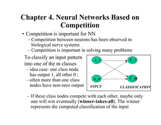
  • 1. Chapter 4. Neural Networks Based on Competition • Competition is important for NN – Competition between neurons has been observed in biological nerve systems – Competition is important in solving many problems To classify an input pattern into one of the m classes – idea case: one class node has output 1, all other 0 ; – often more than one class nodes have non-zero output – If these class nodes compete with each other, maybe only one will win eventually (winner-takes-all). The winner represents the computed classification of the input C_m C_1 x_n x_1 INPUT CLASSIFICATION
  • 2. • Winner-takes-all (WTA): – Among all competing nodes, only one will win and all others will lose – We mainly deal with single winner WTA, but multiple winners WTA are possible (and useful in some applications) – Easiest way to realize WTA: have an external, central arbitrator (a program) to decide the winner by comparing the current outputs of the competitors (break the tie arbitrarily) – This is biologically unsound (no such external arbitrator exists in biological nerve system).
  • 3. • Ways to realize competition in NN – Lateral inhibition (Maxnet, Mexican hat) output of each node feeds to others through inhibitory connections (with negative weights) – Resource competition • output of x_k is distributed to y_i and y_j proportional to w_ki and w_kj, as well as y_i and y_j • self decay • biologically sound • Learning methods in competitive networks – Competitive learning – Kohonen learning (self-organizing map, SOM) – Counter-propagation net – Adaptive resonance theory (ART) in Ch. 5 y_j y_i 0 < ij w y_i y_j x_k kj w ki w 0 < ii w 0 < jj w
  • 4. Fixed-weight Competitive Nets • Notes: – Competition: • iterative process until the net stabilizes (at most one node with positive activation) – where m is the # of competitors • too small: takes too long to converge • too big: may suppress the entire network (no winner) • Maxnet – Lateral inhibition between competitors    > =    − = = otherwise 0 0 if ) ( : function activation otherwise if 1 : weights x x x f j i wij ε ε , / 1 0 m < < ε ε ε ε ε ε
  • 5. Mexical Hat • Architecture: For a given node, – close neighbors: cooperative (mutually excitatory , w > 0) – farther away neighbors: competitive (mutually inhibitory,w < 0) – too far away neighbors: irrelevant (w = 0) • Need a definition of distance (neighborhood): – one dimensional: ordering by index (1,2,…n) – two dimensional: lattice
  • 7. • Equilibrium: – negative input = positive input for all nodes – winner has the highest activation; – its cooperative neighbors also have positive activation; – its competitive neighbors have negative activations. ) 0 . 0 , 39 . 0 , 14 . 1 , 66 . 1 , 14 . 1 , 39 . 0 , 0 . 0 ( ) 2 ( ) 9 . 0 , 38 . 0 , 06 . 1 , 16 . 1 , 06 . 1 , 38 . 0 , 0 . 0 ( ) 1 ( ) 0 . 0 , 5 . 0 , 8 . 0 , 0 . 1 , 8 . 0 , 5 . 0 , 0 . 0 ( ) 0 ( : example = = = x x x
  • 8. Hamming Network • Hamming distance of two vectors, of dimension n, – Number of bits in disagreement. – In bipolar: y x and distance Hamming shorter larger larger ) ( 5 . 0 2 distance hamming and in different bits of number is and in agreement in bits of number is : where ⇒ ⇒ ⋅ + ⋅ = − = ⋅ − = − = ⋅ a y x n y x a n a y x a n d y x d y x a d a y x
  • 9. • Suppose a space of patterns is divided into k classes, each class has an exampler (representative) vector . • An input belongs to class i, if and only if is closer to than to any other , i.e., • Hamming net is such a classifier: – Weights: let represent class j – The total input to j e x x i j e x e x j i ≠ ∀ ⋅ ≥ ⋅ i e j e j Y n b e w j j j 5 . 0 , 5 . 0 = = • j j i i ij j j a n e x x w b in y = + ⋅ = + = ∑ ) ( 2 1 _ j Y
  • 10. • Upper layer: MAX net – it takes the y_in as its initial value, then iterates toward stable state – one output node with highest y_in will be the winner because its weight vector is closest to the input vector • As associative memory: – each corresponds to a stored pattern; – pattern connection/completion; – storage capacity total # of nodes: k total # of patterns stored: k capacity: k (or k/k = 1) j Y
  • 11. • Implicit lateral inhibition by competing limited resources: the activation of the input nodes y_1 y_j y_m x_i i ij j j j i ij ij i ij j x w y y y x w in y in y in y of share larger takes larger ) ( _ _ _ α α β β − ⋅ = = ∑ decay W_ij
  • 12. Competitive Learning • Unsupervised learning • Goal: – Learn to form classes/clusters of examplers/sample patterns according to similarities of these exampers. – Patterns in a cluster would have similar features – No prior knowledge as what features are important for classification, and how many classes are there. • Architecture: – Output nodes: Y_1,…….Y_m, representing the m classes – They are competitors (WTA realized either by an external procedure or by lateral inhibition as in Maxnet)
  • 13. • Training: – Train the network such that the weight vector w.j associated with Y_j becomes the representative vector of the class of input patterns Y_j is to represent. – Two phase unsupervised learning • competing phase: – apply an input vector randomly chosen from sample set. – compute output for all y: – determine the winner (winner is not given in training samples so this is unsupervised) • rewarding phase: – the winner is reworded by updating its weights (weights associated with all other output nodes are not updated) • repeat the two phases many times (and gradually reduce the learning rate) until all weights are stabilized. x j j w x y • ⋅ =
  • 14. x • Weight update: – Method 1: Method 2 In each method, is moved closer to x – Normalizing the weight vector to unit length after it is updated ) ( j j w x w • • − = ∆ α α x w j α α = ∆ • j j j w w w • • • ∆ + = j j j w w w • • • = w_j x x-w_j a(x-w_j) w_j +a(x-w_j) j w• w_j x+w_j w_j+ ax ax
  • 15. • is moving to the center of a cluster of sample vectors after repeated weight updates – Three examplers: S(1), S(2) and S(3) – Initial weight vector w_j(0) – After successively trained by S(1), S(2), and S(3), the weight vector changes to w_j(1), w_j(2), and w_j(3) j w• S(2) S(1) S(3) w_j(0) w_j(1) w_j(2) w_j(3)
  • 16. Examples • A simple example of competitive learning (pp. 172-175) – 4 vectors of dimension 4 in 2 classes (4 input nodes, 2 output nodes) S(1) = (1, 1, 0, 0) S(2) = (0, 0, 0, 1) S(3) = (1, 0, 0, 0) S(4) = (0, 0, 1, 1) – Initialization: , weight matrix: – Training with S(1) 6 . 0 = α α             = 3 . 9 . 7 . 5 . 4 . 6 . 8 . 2 . W 86 . 1 ) 0 9 (. ) 0 5 (. ) 1 6 (. ) 1 2 (. ) 1 ( ) 1 ( 2 2 2 2 1 = − + − + − + − = − = • w S D wins 2 class , 98 . 0 ) 1 ( ) 1 ( 2 = − = • w S D             =             −             +             = • 12 . 28 . 76 . 92 . ) 3 . 7 . 4 . 8 . 0 0 1 1 ( 6 . 0 3 . 7 . 4 . 8 . 2 w             = 12 . 9 . 28 . 5 . 76 . 6 . 92 . 2 . then W
  • 17. – Similarly, after training with S(2) = (0, 0, 0, 1) , in which class 1 wins, weight matrix becomes – At the end of the first iteration (each of the 4 vectors are used), weight matrix becomes – Reduce – Repeat training. After 10 iterations, weight matrix becomes 3 . 0 6 . 0 5 . 0 5 . 0 = ⋅ = ⋅ = α α α α             = 12 . 96 . 28 . 20 . 76 . 24 . 92 . 08 . W             = 048 . 980 . 110 . 680 . 300 . 096 . 970 . 032 . W α α             →             − − − − = 0 . 0 0 . 1 0 . 0 5 . 0 5 . 0 0 . 0 0 . 1 0 . 0 16 0 . 1 000000 . 1 16 3 . 2 5100000 . 4900000 . 16 0 . 2 000000 . 1 17 7 . 6 e e e e W • S(1) and S(3) belong to class 2 • S(2) and S(4) belong to class 1 • w_1 and w_2 are the centroids of the two classes
  • 18. Comments 1. Ideally, when learning stops, each is close to the centroid of a group/cluster of sample input vectors. 2. To stabilize , the learning rate may be reduced slowly toward zero during learning. 3. # of output nodes: – too few: several clusters may be combined into one class – too many: over classification – ART model (later) allows dynamic add/remove output nodes 4. Initial : – training samples known to be in distinct classes, provided such info is available – random (bad choices may cause anomaly) j w• j w• α α j w•
  • 19. Example will always win no matter the sample is from which class is stuck and will not participate in learning unstuck: let output nodes have some conscience temporarily shot off nodes which have had very high winning rate (hard to determine what rate should be considered as “very high”) 2 • w 1 • w w_1 w_2
  • 20. Kohonen Self-Organizing Maps (SOM) • Competitive learning (Kohonen 1982) is a special case of SOM (Kohonen 1989) • In competitive learning, – the network is trained to organize input vector space into subspaces/classes/clusters – each output node corresponds to one class – the output nodes are not ordered: random map w_3 w_2 cluster_1 cluster_3 cluster_2 w_1 • The topological order of the three clusters is 1, 2, 3 • The order of their maps at output nodes are 2, 3, 1 • The map does not preserve the topological order of the training vectors
  • 21. • Topographic map – a mapping that preserves neighborhood relations between input vectors, (topology preserving or feature preserving). – if are two neighboring input vectors ( by some distance metrics), – their corresponding winning output nodes (classes), i and j must also be close to each other in some fashion – one dimensional: line or ring, node i has neighbors or – two dimensional:grid. rectangular: node(i, j) has neighbors: hexagonal: 6 neighbors 2 and 1 x x 1 ± i )) 1 , 1 ( additional or ( ), , 1 ( ), 1 , ( ± ± ± ± j i j i j i n i mod 1 ±
  • 22. • Biological motivation – Mapping two dimensional continuous inputs from sensory organ (eyes, ears, skin, etc) to two dimensional discrete outputs in the nerve system. • Retinotopic map: from eye (retina) to the visual cortex. • Tonotopic map: from the ear to the auditory cortex – These maps preserve topographic orders of input. – Biological evidence shows that the connections in these maps are not entirely “pre-programmed” or “pre-wired” at birth. Learning must occur after the birth to create the necessary connections for appropriate topographic mapping.
  • 23. SOM Architecture • Two layer network: – Output layer: • Each node represents a class (of inputs) • • Neighborhood relation is defined over these nodes Each node cooperates with all its neighbors within distance R and competes with all other output nodes. • Cooperation and competition of these nodes can be realized by Mexican Hat model R = 0: all nodes are competitors (no cooperative) à random map R > 0: à topology preserving map ∑ = ⋅ = • i i ij j j x w w x y : activation Node
  • 24. SOM Learning 1. Initialize , and to a small value 2. For a randomly selected input sample/exampler determine the winning output node J either is maximum or is minimum 3. For all output node j with , update the weight 4. Periodically reduce and R slowly. 5. Repeat 2 - 4 until the network stabilized. x J W x • ⋅ ∑ − = − • i i ij J x w w x 2 ) ( R j J ≤ − ) ( ij ij ij w x w w − + = α α α α nodes output all for j W• α α
  • 25. Notes 1. Initial weights: small random value from (-e, e) 2. Reduction of : Linear: Geometric: may be 1 or greater than 1 3. Reduction of R: should be much slower than reduction. R can be a constant through out the learning. 4. Effect of learning For each input x, not only the weight vector of winner J is pulled closer to x, but also the weights of J’s close neighbors (within the radius of R). 5. Eventually, becomes close (similar) to . The classes they represent are also similar. 6. May need large initial R α α α α α α α α ∆ − = ∆ + ) ( ) ( t t t β β α α α α ) ( ) ( t t t = ∆ + t ∆ 0 ) ( while 1 ) ( ) ( > − = ∆ + t R t R t t R α α j w• 1 ± • j w
  • 26. Examples • A simple example of competitive learning (pp. 172-175) – 4 vectors of dimension 4 in 2 classes (4 input nodes, 2 output nodes) S(1) = (1, 1, 0, 0) S(2) = (0, 0, 0, 1) S(3) = (1, 0, 0, 0) S(4) = (0, 0, 1, 1) – Initialization: , weight matrix: – Training with S(1) 6 . 0 = α α             = 3 . 9 . 7 . 5 . 4 . 6 . 8 . 2 . W 86 . 1 ) 0 9 (. ) 0 5 (. ) 1 6 (. ) 1 2 (. ) 1 ( ) 1 ( 2 2 2 2 1 = − + − + − + − = − = • w S D wins 2 class , 98 . 0 ) 1 ( ) 1 ( 2 = − = • w S D             =             −             +             = • 12 . 28 . 76 . 92 . ) 3 . 7 . 4 . 8 . 0 0 1 1 ( 6 . 0 3 . 7 . 4 . 8 . 2 w             = 12 . 9 . 28 . 5 . 76 . 6 . 92 . 2 . then W
  • 27. • How to illustrate Kohonen map – Input vector: 2 dimensional Output vector: 1 dimensional line/ring or 2 dimensional grid. Weight vector is also 2 dimension – Represent the topology of output nodes by points on a 2 dimensional plane. Plotting each output node on the plane with its weight vector as its coordinates. – Connecting neighboring output nodes by a line output nodes: (1, 1) (2, 1) (1, 2) weight vectors: (0.5, 0.5) (0.7, 0.2) (0.9, 0.9) C(1, 2) C(2, 1) C(1, 1)
  • 28. Traveling Salesman Problem (TSP) by SOM • Each city is represented as a 2 dimensional input vector (its coordinates (x, y)), • Output nodes C_j form a one dimensional SOM, each node corresponds to a city. • Initially, C_1, ... , C_n have random weight vectors • During learning, a winner C_j on an input (x, y) of city I, not only moves its w_j toward (x, y), but also that of of its neighbors (w_(j+1), w_(j-1)). • As the result, C_(j-1) and C_(j+1) will later be more likely to win with input vectors similar to (x, y), i.e, those cities closer to I • At the end, if a node j represents city I, it would end up to have its neighbors j+1 or j-1 to represent cities similar to city I (i,e., cities close to city I). • This can be viewed as a concurrent greedy algorithm
  • 29. Initial position Two candidate solutions: ADFGHIJBC ADFGHIJCB
  • 31.
  • 32. Counter propagation network (CPN) • Basic idea of CPN – Purpose: fast and coarse approximation of vector mapping • not to map any given x to its with given precision, • input vectors x are divided into clusters/classes. • each cluster of x has one output y, which is (hopefully) the average of for all x in that class. – Architecture: Simple case: FORWARD ONLY CPN, ) (x y φ φ = ) (x φ φ ) (x φ φ m p n k j j j i y z x y w z v x y z x 1 1 1 • • from (input) features to class from class to (output) features
  • 33. – Learning in two phases: – training sample x:y where is the precise mapping – Phase1: is trained by competitive learning to become the representative vector of a cluster of input vectors x (use sample x only) 1. For a chosen x, feedforward to determined the winning 2. 3. Reduce , then repeat steps 1 and 2 until stop condition is met – Phase 2: is trained by delta rule to be an average output of where x is an input vector that causes to win (use both x and y). 1. For a chosen x, feedforward to determined the winning 2. (optional) 3. 4. Repeat steps 1 – 3 until stop condition is met ) (x y φ φ = j v• • j w ) (x φ φ j z j z )) ( ( ) ( ) ( old v x old v new v ij i ij ij − + = α α α α )) ( ( ) ( ) ( old v x old v new v ij i ij ij − + = α α )) ( ( ) ( ) ( old w y old w new w jk k jk jk − + = α α j z
  • 34. • A combination of both unsupervised learning (for in phase 1) and supervised learning (for in phase 2). • After phase 1, clusters are formed among sample input x , each is a representative of a cluster (average). • After phase 2, each cluster j maps to an output vector y, which is the average of • View phase 2 learning as following delta rule • Notes j v• • j w j v• { } : ) ( j cluster x x ∈ φ φ wins when ) ( 2 ) ( because , where ) ( 2 j j jk k j jk k jk jk jk jk k jk k jk jk z z w y z w y w w E w E w y w y w w − − = − ∂ ∂ = ∂ ∂ ∂ ∂ − ∝ − − + = ∑ α α win make that samples training all of mean the is where ) ( ) ( and ) ( , when , shown that be can It x x x t w x t v t j j φ φ → → ∞ → • •
  • 35. ) 1 ( ) ( ) 1 ( ) 1 ( as rewriteen be can rule update Weight similar.) is of (proof on only Show + + − = + t x t v t v w v i ij ij jk ij α α α α [ ] t i i i i i i ij i i ij i ij ij x t x t x t x t x t x t v t x t x t v t x t v t v ) 1 )( 1 ( ... ) 1 )( 1 ( ) 1 )( ( ) 1 ( ) 1 ( ) ( ) 1 ( ) 1 ( ) 1 ( ) 1 ( )) ( ) 1 ( ) 1 )(( 1 ( ) 1 ( ) ( ) 1 ( ) 1 ( 2 2 α α α α α α α α α α α α α α α α α α α α α α α α α α α α − + − − + − + + ≈ + + − + − − = + + + − − − = + + − = + x x x x E t x E t x E x t x t x E t v E t i t t i i ij = − − ⇒ − + − + = − + − + + = − + − + + = + ) 1 ( 1 1 ] ) 1 ....( ) 1 ( 1 [ ))] 1 ( ( ) 1 ...( )) ( ( ) 1 ( )) 1 ( ( [ ] ) 1 ( ... ) 1 )( ( ) 1 ( ( [ )] 1 ( [ 1 α α α α α α α α α α α α α α α α α α α α α α then set, training the from randomly drawn are If x
  • 36. • After training, the network works like a look-up of math table. – For any input x, find a region where x falls (represented by the wining z node); – use the region as the index to look-up the table for the function value. – CPN works in multi-dimensional input space – More cluster nodes (z), more accurate mapping.
  • 37. • If both we can establish bi-directional approximation • Two pairs of weights matrices: V ( ) and U ( ) for approx. map x to W ( ) and T ( ) for approx. map y to • When x:y is applied ( ), they can jointly determine the winner J or separately for • pp. 196 –206 for more details exist ) ( function inverse its and ) ( 1 y x x y − = = φ φ φ φ z x to ) (x y φ φ = ) ( * x x φ φ = Y y X x on and on Jy Jx z z , Full CPN y z to z y to x z to