Volume 18, Issue 3, Ver. IV (May-Jun. 2016)

1. IOSR Journal of Computer Engineering (IOSR-JCE)
e-ISSN: 2278-0661,p-ISSN: 2278-8727, Volume 18, Issue 3, Ver. IV (May-Jun. 2016), PP 110-115
www.iosrjournals.org
DOI: 10.9790/0661-180304110115 www.iosrjournals.org 110 | Page
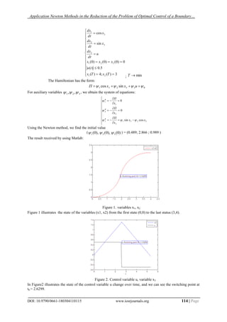
Application Newton methods in the reduction of the problem of
optimal control of a boundary value problem.
Dang Thi Mai1
, Nguyen Viet Hung2
1
(Department of Basic Science, University of Transport and Communications, Lang Thuong, Dong Da,
Ha Noi, Viet Nam,)
2
(Le Quy Don Technical University)
Abstract : The article presents a generalized continuation of the parameter and Newton methods for solving
nonlinear equations . It describes and explores one approach to the application of the continuation method for
solving boundary value problems when searching for the optimal control. Solving boundary using the parameter
and the solution obtained in the choice of variables. The results of simulations performed on Matlab.
Keywords: method Newton; boundary value problems; the parameter
I. Introduction
Consider a system of nonlinear algebraic and transcendental equations n in the unknowns x1, x2, …, xn
containing parameter p:
.0),( pxF . .1((1)
Here  T
nxxxx )...,,,( 21 the vector, p
1
R and  T
nFFFF ),...,,( 21 the vector valued function in
space Rn
.
Suppose that for some values 0pp  , known solution       )0(02010 ,...,, nxxxx  , equation (1), ie,
  .0),( 00 pxF (2)
Consider the neighborhood of U  
1
00 ),( 
 n
Rpx in the form of a cuboid with the center in point   ),( 00 px .
The implicit function theorem.
Theorem 1. ([1]) Suppose that,
1. The vector function F is defined and continuous in U   ),( 00 px .
2. In U exist continuous partial derivatives of F with respect to ),1( niFi  all arguments ),1( nixi  and the
parameter p.
3. Point   ),( 00 px satisfies (1).
4. At point   ),( 00 px is nonzero Jacobian det ( J ), whose matrix is of the form:
 
 















































n
nnn
n
n
n
n
x
F
x
F
x
F
x
F
x
F
x
F
x
F
x
F
x
F
xx
FF
x
F
J




21
2
2
2
1
2
1
2
1
1
1
1
1
,...,
,..., (3)
Then in a neighborhood of (x(0), p0) of equations (1) defines x1, x2,…,xn as a single-valued functions p
nipxx ii ,1),(  (4)
features (4) satisfy the conditions of xi(p0) = xi(0), i = 1,2,..,n and dxi /dp (i=1,2,..,n) derivatives are also
continuous in this neighborhood.
Hence, the implicit function theorem defines a neighborhood of U single curve point (x(0), p0), which has a
parametric representation (4). This curve is called the curve of the set of solutions of the equations (1).
The first and third conditions of Theorem 1 is not very burdensome.
The points at which det(J) nonzero (3) will be called regular, and the points where det (J) = 0 – special.

2. Application Newton Methods in the Reduction of the Problem of Optimal Control of a Boundary…
DOI: 10.9790/0661-180304110115 www.iosrjournals.org 111 | Page
The singular points of the continuation of the solution may be mixed, ie there is a plurality of branching of
solutions of (1), if may be possible to continue making.
The first use of the idea of continuing in computer belongs to, apparently, M. Laeyu [2]. He introduced the
transcendental equation H(x) = 0 parameter p and thus reduced it to an equation of the form (1). And the option
has been introduced so that for p= p0 = 0, we can easily obtain the solution x0=x(p0), and when p=pk= 1, the
equation would be applied to the original. Going by the sequence of values of the parameter p0 < p1 <…< pk, M.
Laeyu proposed to build a solution for every pi, i=1,2…,k by using Newton-Raphson method, use the solution
for the previous pi-1 values as an initial approximation.
)()()(
)( i
jj
i pxx  denote the approximate value of the desired solution )()( ii pxx  to the j-th step of the
iterative process of Newton-Raphson method at ipp  . Then proposed by M. Laeyu process of constructing
the solution of equation (1) in the transition from pi-1 to pi can be written as:
   
,.....2,1
,,, )1(
)(
)1(
)(
1)1(
)(
)(
)(
),1(
)0(
)(





j
pxFpxJxx
xx
i
j
ii
j
i
j
i
j
i
ii
(5)
where 
),( )1(
)(
1
i
j
i pxJ inverse Jacobi (3) when i
j
i ppxx  
,)1(
)(
The iterative process (5) is carried out to satisfy the condition   )1(
)(
)(
)(
j
i
j
i xx , where 0 given the
accuracy of calculations.
II. A continuous analogue of Newton's method
Another formulation of the continuation method have DF Davidenko [3, 4]. Differentiating system (1) as a
complex function of the parameter p
 .)(,,0 00 xpx
x
F
J
p
F
dp
dx
J 





 (6)
For this system of equation (1) is complete integral satisfying the condition    0, 00 pxF .
The system of equations (6) is linear in the derivatives dpdx/ . Provided non-zero determinant of the
Jacobian J arrive at a system of ordinary differential equations
   00
1
,)( xpx
p
F
xJ
dp
dx



  (7)
The system of equations of this problem is called a continuation of the equations in normal form.
This approach solves the problem of the choice of the initial approximation to the solution. The
simplest of these schemes, the method of the Euler scheme when, leads to the following algorithm:
 
       
,1,0
,),(,)(
1
1
00








ki
ppx
p
F
pxJxx
xx
iiiiii
(8)
where .1 ii ppp  
Continuation of solutions by integrating the Cauchy problem is commonly called a continuous analogue of
Newton.
We now note one interesting possibility of using the continuation method established by MK Gavurin [5].
To solve nonlinear equations construct an equation with the parameter as follows
 1,0,0)()1()(),( )0(  pxHpxHpxF (9)
Here, the parameter p is entered so that a solution of equation (9) with p = 0 and p = 1, the equation refers
to the original. If we now enter a new parameter λ so that
  
,0,1 
ep (10)
then the equation (9) takes the form:
0)()(),( )0(  
xHexHxF 
 (11)
Differentiation of this equation for λ leads to the following Cauchy problem in the parameter λ.
.)0(),( )0(
1
xxxH
x
H
d
dx











(12)
Integration is the task for λ Euler method with step 1 leads to the iterative process

3. Application Newton Methods in the Reduction of the Problem of Optimal Control of a Boundary…
DOI: 10.9790/0661-180304110115 www.iosrjournals.org 112 | Page
 
 
,...2,1,0,
,
)(
)0(
0
)(
1
)()1(












jxx
xH
x
xH
xx j
j
jj
(13)
But this process is exactly the same as the process of iterative Newton-Raphson method for the equation H
(x) = 0 for the initial approximation .)0(
)0(
xx 
Continuation method on parameter in the form presented here can be little or no change in the common
non-linear operator equations, if by ),( pxF understand non-linear invertible operator with a parameter.
III. Generalized to the solution continuously variable
A boundary value problem:
 
nnn
n RfRxRbbbB
TtBTxtxfx


,;),...,,(
,,0,)(),,(
21

(14)
must select
  ).,...,,(,0 21 naaaAAx  (15)
Thus, to satisfy the boundary conditions.
Here it is assumed that the boundary problem (14) - (15) has a unique solution.
We introduce the functional
 

n
i
ii bTxAT
1
2
)(),( (16)
Minimum functional ),( AT on a set of initial values   Ax 0 (15) determines the solution of the boundary
problem (14) - (15).
We calculate the minimum functionality specified by Newton's formula:
 
)0(
,...2,1),()(
0
1
1
xA
kAAAA kkkk

 

 (17)
Where  )( kA the gradient of the function ),( AT at the   )(, kk AA Hessian matrix.
We now divide the interval of integration [0, T] on a system of nested segments:
       Tttt r ,0,0,0,0 21   (18)
On the segment  1,0 t we define the functional form (16) with the substitution T is t1:
 

n
i
ii btxAt
1
2
11 )(),( (19)
Since the segment [0, t1] is small, the minimum of the functional (19) is easily found by Newton's formula
(17).
Next on the interval [0,t2] we consider the minimum of the functional (16) with the substitution therein T to t2,
using as a first approximation of the solution obtained on the interval [0, t1]. This process can continue until the
tr = T.
It should be noted that the proposed procedure removed the question of the choice of the initial
approximation in an iterative Newton process (17). However, the convergence of the proposed method is
determined by conditioning Hessian. When bad conditionality growing number of partitions of the interval [0,
T], which in turn leads to a decrease in the efficiency of the method and the growth of rounding errors.
IV. Reduction of the problem of optimal control of a boundary value problem.
It is known that the problem of finding extremals in Pontryagin optimal control problem is reduced to
solving boundary value problem, it can be used to her numerical methods described above. Next, a class of
optimal control problems, the process of constructing a boundary value problem and the features of the
application to her continuation method.
We write down the standard formulation of the optimal control problem. Let's start with performance
problems in the presence of the end manifolds:
min
,)(,)0(
,),,,(
10



T
XTxXx
RUuRxtuxfx mn

(20)
where control )(u belongs to the class of piecewise continuous functions.

4. Application Newton Methods in the Reduction of the Problem of Optimal Control of a Boundary…
DOI: 10.9790/0661-180304110115 www.iosrjournals.org 113 | Page
To find the extremal problem will apply the necessary condition for optimality in the form of the Pontryagin
maximum principle. We write the function of the Hamilton-Pontryagin:
 ),,,(),,,( tuxftuxП  (21)
Assumption 4.1. The optimal control for the problem (20) exists.
Obviously, this assumption is satisfied (a consequence of the convexity of the management) for tasks that
are affine in control.
Assuming that the maximum principle requirements are met, the corresponding theorem guarantees the
existence of a nontrivial conjugate variable ѱ, which satisfies the adjoint equation, which in combination with
the original differential system gives the boundary value problem for the maximum principle:
)),,,(,,(
),),,,(,,(
*
*
ttxuxП
ttxuxПx
x 





(22)
The boundary conditions are obtained from the environment:
.)(,)0( 10 xTxxx  (23)
For problems with non-fixed time, such as performance problems, it is proposed to make the change to the
time variable
T
t
 , and enter the time T in the phase space of a constant function:
 .1,0,0),),,,(,,(
),),,,(,,(
*
*






TxuxTП
xuxTПx
x


To eliminate the ambiguity associated with the invariance of the conjugate variable to multiplication by a
constant need to take the normalization condition of the conjugate variable at one end by-cutting. Thus, we have
2n + 1 ordinary differential equations and the same boundary conditions.
For problems with the terminal functionality min))((  TxFJ is changed only the right boundary
condition: )).(()( TxFT 
For the purposes of an integral functional:
 
T
dtttutxfJ
0
0 min)),(),((
Changes Hamilton-Pontryagin
 ),,,(),,,( tuxftuxП  + )),(),((00 ttutxf
assuming the existence of a functional, can be put 10  . In the case of non-fixed the right end of the
boundary condition on the right end 1)( xTx  is replaced by .0)( T
To apply the continuation method, described in the previous section, to put boundary value problems is
necessary to put forward additional conditions: It requires the existence of continuous derivatives
      )(,,,,, **
00 uuffff xxuxuxxxx
. For tasks that are affine in control, provided the regularity of the
control system, ie, nondegeneracy gradient 0),,(  txПu  , can be found analytically ),,(*
txu 
),,(
)(
txП
U
u
s






, where  ,max)( us
Uu
U

 .
Until now, the assumption was made that the operating area is sleek and compact. Otherwise (eg rectangle)
application of the method of continuation on parameter directly is impossible, since it is not provided with the
requirements of the existence of continuous derivatives maximizer, and therefore violated the assumption of
smoothness and regularity.
To avoid these difficulties, the application of smoothing management. Details smoothing convex compacts
described in [8]. Investigation of stability of solutions of the optimal control problem for smoothing the
management is given in [9].
V. Example and numerical result
The Newton method is used to find the initial value for the boundary value problem, and then applied to the
solution of optimization problems quick impact
Example 1.

5. Application Newton Methods in the Reduction of the Problem of Optimal Control of a Boundary…
DOI: 10.9790/0661-180304110115 www.iosrjournals.org 114 | Page




















3)(;4)(
5.0)(
0)0()0()0(
sin
cos
21
321
3
3
2
3
1
TxTx
tu
xxx
u
dt
dx
x
dt
dx
x
dt
dx
; minT
The Hamiltonian has the form:
033231 sincos   uxxП
For auxiliary variables 321 ,,  , we obtain the system of equations:
























3231
3
3
2
2
1
1
cossin
0
0
xx
x
П
x
П
x
П



Using the Newton method, we find the initial value
( )0(),0(),0( 321  ) = (0.489; 2.866 ; 0.989 )
The result received by using Matlab:
Figure 1. variables x1, x2
Figure 1 illustrates the state of the variables (x1, x2) from the first state (0,0) to the last status (3,4).
Figure 2. Control variable u, variable x3
In Figure2 illustrates the state of the control variable u change over time, and we can see the switching point at
t0 = 2.6299.

6. Application Newton Methods in the Reduction of the Problem of Optimal Control of a Boundary…
DOI: 10.9790/0661-180304110115 www.iosrjournals.org 115 | Page
The results obtained:
9837.2)(;9998.3)(;3899.5 21  TxTxT
References
[1]. Л.Д. Кудрявцев. Математический анализ. т.2. М.: Высшая школа, 1973.
[2]. Д. Ортега, В.Рейнболдт. Итерационные методы решения нелинейных систем уравнений
со многими неизвестными. М.: Мир. 1975.
[3]. Д.Ф. Давиденко. Об одном новом методе численного решения систем нелинейных уравнений
// ДАН СССР. 1953. Т.88. №4. С. 601-602.
[4]. Д.Ф. Давиденко. О приближенном решении систем нелинейных уравнений // Укр. мат. журн.
1953, Т.5.№2. С. 196-206.
[5]. М.К. Гавурин. Нелинейные функциональные уравнения и непрерывные аналоги итеративных
методов // Изв. Вузов. Математика. 1958. №5. С. 18-31.
[6]. В.И.Шалашилин, Е.Б.Кузнецов. метод продолжения по параметру и наилучшая
параметризация. Москва, 1999.
[7]. С.С.Жулин. Метод продолжения решения по параметру и его приложение к задачам
оптимального управления. В.Ц 2007 и Т.8.
[8]. Аввакумов СИ. Гладкая аппроксимация выпуклых компактов // Тр. Ин-та матем. и механ.
УрО РАН. Ека теринбург. 1996. 4. 184-200.
[9]. Аввакумов С.Н., Киселев Ю.Н., Орлов М.В. Методы решения задач оптимального
управления на основе принципа максимума Понтрягина // Тр. Матем. ин-та им. В. А. Стеклова
РАН. 1995. 211. 3-31.