The document discusses quantitative analysis of 3D refractive index maps obtained from Nanolive's 3D Cell Explorer microscope. It describes using the software FIJI to extract numerical features from segmented objects in the maps, such as volume, surface area, and compactness of HeLa cell nuclei. It also demonstrates advanced segmentation of mouse embryonic stem cells and quantitative analysis of cell volume and dry mass changes during cell division.

1. Quantitative Analysis of 3D Refractive Index Maps
Nanolive SA
Chemin de la Dent d‘Oche 1a | 1024 Ecublens | Switzerland
Application Note by Nanolive SA

2. Application Note by Nanolive SA
1
Abstract
Nanolive’s 3D Cell Explorer allows for the creation of high-content 3D images of living cells with very
high spatio-temporal resolution (x, y:180nm; z:400nm; t:1.7sec). Being able to extract quantitative
data describing the objects (population of cells, cells, organelles) contained in such images is at
the core of leading-edge cell biology research. This application note will start where application
note 2 (AppNote2017-2) stopped by looking at how meaningful numbers can be extracted from
segmented objects using FIJI. We will then bring some cellular features in perspective to help you to
start elegant quantitative studies with the 3D Cell Explorer.

3. Application Note by Nanolive SA
2
1. Introduction
The 3D Cell Explorer allows to acquire a three-dimensional map of the refractive index (RI) composing
your objects of interest (Cotte et al., 2013). The finesse of the device allows to observe differences
of RI as small as 0.001, by far the best sensitivity on the market, thus providing a fine view of the
different elements composing a sample, such as the different compartments of a cell for example.
Consequently, even a non-expert would be able to identify by eye the nucleus of a mammalian cell
in an RI map. However, at the age of quantitative cell biology (Langen et al., 2015; Li et al., 2007)
where seeing, feeling and manual image analysis is no more the norm, it is crucial that the computer
crunches your image to extract meaningful object features organized in space, time and object
identity (Frechin et al., 2015). The goal of this application note is to demonstrate how to obtain a
set of numerical features that will describe your objects of interest once they have been segmented
(See AppNote2017-2). We will use two examples to illustrate the use of FIJI for extracting quantitative
data based on sets of 3D segmented objects. The two examples will concern i) HeLa cell nuclei and ii)
a time series of mouse embryonic stem cell images. This will require the software FIJI (Schindelin et
al., 2012; Schmid, Schindelin, Cardona, Longair, & Heisenberg, 2010; Schneider, Rasband, & Eliceiri,
2012) and the software STEVE (http://nanolive.ch/software/#trySteve). We will see how to extract
a large panel of features from an object as well as simple visualization cases, more advanced 3D
object segmentation and feature plotting with a focus on how to calculate dry mass out of refractive
index values. Please keep in mind that the parameters and procedures shown here are no rule of
thumb and should be carefully evaluated before applying them to your specific problem.
2. Prerequisites
First, you will need the latest version of STEVE (http://nanolive.ch/software/#trySteve), the software
that allows to control your 3D Cell Explorer, and second, the latest version of FIJI (http://fiji.
sc/#download) with the 3D ImageJ suite (See AppNote2017 1 or 2).
Figure 1: Setup of the 3D manager options

4. Application Note by Nanolive SA
3
Application Note by Nanolive SA
This application note starts exactly where AppNote2017-2 stopped. Thus, you should launch
the latest version of FIJI and load the stack of 3D segmented HeLa nuclei. Follow the procedure
described in Figure 1 to set up the 3D manager options. This set of options will ensure that your
first calculations are processed quickly. Only a few measurements will be requested later such as
the volume and surface of each object, expressed in voxels, as well as the compactness that gives
information on how spherical an object is (from 0 to 1).
3. Using the 3D manager with segmented objects
The 3D manager is certainly the best free 3D object analysis tool, and it is very easy to use (for a
complete manual of the 3D analysis suite of ImageJ see: https://goo.gl/syLkaG). To visualize the
stack of segmented nuclei in 3D, click on the stack that you want to see in 3D, then go to Plugins >
3D Viewer (Figure 2, step 1). To analyze these objects, go to Plugins > 3D > 3D manager (Figure 2,
step 2). A window opens, click on the segmentation stack and then click on the AddImage button
(Figure 2, step 3). This action will load the objects contained in the segmented image. Click now on
the Distances button. This action creates a table that lists various distances between each object
such as centroid to centroid or edge to edge distances (Figure 2, step 4). Figure 3 shows a selection
of features given by the Distances and Measure 3D functionalities of the 3D manager plugin. The
tool provides measurements in voxels and conversion to µm2 or µm3 is done by considering the
dimensions of a single voxel in x,y,z which are 0.186, 0.186 and 0.372 µm.
You can increase the number of features that are returned by the 3D manager by changing the 3D
manager options (Figure 1).
Figure 2: Using the 3D manager

5. Application Note by Nanolive SA
4
4. Advanced segmentation using MorphoLibJ
We will now look at a slightly more advanced segmentation of mouse embryonic stem cells. This
procedure follows the same procedure as exposed in the A p p N o t e 2 0 1 7 – 2. Instead of segmenting
nuclei, we segment entire cells here. While nuclei could be segmented using a simple segmentation
based on thresholding (Plugins > 3D > 3D Simple Segmentation, see AppNote2017-2), we use here
the MorphoLibJ plugin. Follow the installation procedure of the plugin: Help > Update > Manage
update sites and tick IJPB-plugins, close and apply changes.
Follow the procedure shown in Figure 4 to open the morphological segmentation tool (Figure 4,
step 1-4). As a starting point for your specific case, we recommend clicking object image (unless
you have a border image you already derived from your original image) to leave the gradient radius
on 1 (parameter used to detect object borders) and the tolerance on 10 (minimal distance to detect
successive maxima in the image). Click Run and see what happens. This turns out to be an excellent
starting point for 3D Cell Explorer images in general (Figure 4, step 5 and 6). You can then create
Figure 3: Extraction of HeLa nuclei features
Figure 4: MorphoLibJ: morphological segmentation allows for a more advanced segmentation
Four HeLa cells : cytosol + DNA 3D segmented nuclei
Visualisation with Tomviz 3D segmentation with FIJI
1
2 3
4
Object
1
2
3
4
Volume Surface Compactness
17.8 μm
13.3 μm
14 μm
15.8 μm 902
μm3 μm2
951
1380
1070
553
493
633
560
0.4
0.6
0.63
0.55
Sphere = 1

6. Application Note by Nanolive SA
5
an image out of Catchment bassins (Figure 4, step 7). You will then need to transform it into
grayscale to be able to use it back as a normal segmented image. To do so, click on Image > Type >
8bit after selecting the colored image you just produced. The usage of such a tool certainly requires
time to find the proper parameters to obtain the desired results.
5.Exampleofquantitative analysisofmouseembryonicstemcellsdivision
Figure 5: Analysis of cell volume and dry mass of two dividing mESCs

7. Application Note by Nanolive SA
6
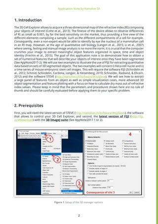
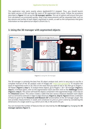
It is very easy to extract information from another image such as a 3D refractive index map if a specific
3D segmentation has been made. Load your 3D segmentation in the 3D manager as described in
Figure 2 in paragraph 3. Then, open the image from which you want to extract information (the 3D
refractive index map). This image must have the same size as the segmented image. Select it as the
active window by clicking on it, then go on the 3D manager window and click on Quantif 3D. The
table that opens lists all the required measures, one line per object contained in the segmentation
image you loaded first. The features that can be returned by Quantif 3D are those related to gray
values in the 3D manager options panel. By making adjustments, you will get a feel of it and will
certainly obtain the results you are looking for.
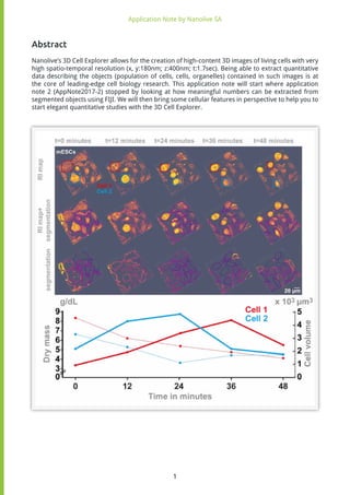
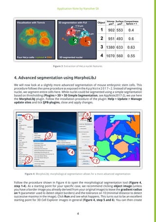
The analysis displayed in Figure 5 illustrates mouse Embryonic Stem Cells (mESCs) imaged over 48
minutes with the 3D Cell Explorer. The cells in the recorded images have been segmented following
previously described procedures (see AppNote2017-2 and paragraph above) to be able to extract
not only the volume but also the refractive index values of each object. The dry mass of each object
has then been calculated using the following formula (Friebel & Meinke, 2006; Phillips, Jacques, &
McCarty, 2012):
[DryMass] =
where
k = 0.002
for material that has no specific light absorbance characteristic.
Those values are then plotted as a function of time, for two cells that undergo mitosis one after the
other. One can observe that the concentration of cellular dry mass increases during mitosis, and
decreases afterwards. Yet interestingly, the volume of those cells is still relatively small when the
dry mass concentration starts decreasing, suggesting an active loss of cellular material during the
post cytokinesis times.
6. General Hardware & Software Requirements
3D Cell Explorer models:
3D Cell Explorer
3D Cell Explorer-fluo
Software:
STEVE – all versions
FIJI with the 3D ImageJ suite
RI
RIH2O
1
k
− 1 ×

8. Application Note by Nanolive SA
7. References
Cotte, Y., Toy, F., Jourdain, P., Pavillon, N., Boss, D., Magistretti, P., … Depeursinge, C. (2013).
Marker-free phase nanoscopy. Nature Photonics, 7(2), 113–117.
Frechin, M., Stoeger, T., Daetwyler, S., Gehin, C., Battich, N., Damm, E.-M., … Pelkmans, L. (2015).
Cell-intrinsic adaptation of lipid composition to local crowding drives social behaviour.
Nature, 523(7558), 88–91. https://doi.org/10.1038/nature14429
Friebel, M., & Meinke, M. (2006). Model function to calculate the refractive index of native hemoglobin
in the wavelength range of 250-1100 nm dependent on concentration.
Applied Optics, 45(12), 2838. https://doi.org/10.1364/AO.45.002838
Langen, M., Agi, E., Altschuler, D. J., Wu, L. F., Altschuler, S. J., & Hiesinger, P. R. (2015). The
Developmental Rules of Neural Superposition in Drosophila.
Cell, 162(1), 120–133. https://doi.org/10.1016/j.cell.2015.05.055
Li, G., Liu, T., Tarokh, A., Nie, J., Guo, L., Mara, A., … Wong, S. T. (2007). 3D cell nuclei segmentation
based on gradient flow tracking.
BMC Cell Biology, 8(1), 40. https://doi.org/10.1186/1471-2121-8-40
Phillips, K. G., Jacques, S. L., & McCarty, O. J. T. (2012). Measurement of Single Cell Refractive Index,
Dry Mass, Volume, and Density Using a Transillumination Microscope.
Physical Review Letters, 109(11). https://doi.org/10.1103/PhysRevLett.109.118105
Schindelin, J., Arganda-Carreras, I., Frise, E., Kaynig, V., Longair, M., Pietzsch, T., … Cardona, A. (2012).
Fiji: an open-source platform for biological-image analysis.
Nature Methods, 9(7), 676–682. https://doi.org/10.1038/nmeth.2019
Schmid, B., Schindelin, J., Cardona, A., Longair, M., & Heisenberg, M. (2010). A high-level 3D
visualization API for Java and ImageJ.
BMC Bioinformatics, 11(1), 274. https://doi.org/10.1186/1471-2105-11-274
Schneider, C. A., Rasband, W. S., & Eliceiri, K. W. (2012). NIH Image to ImageJ: 25 years of image
analysis. Nature Methods, 9(7), 671–675. https://doi.org/10.1038/nmeth.2089
A p p N o t e 2 0 1 7 - 3