Download to read offline


![Monte Carlo model
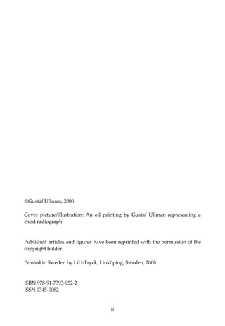
3.2.2.3 Scattered photons and variance reduction techniques
The simulation of scattered photons is time consuming. Therefore, different
variance reduction techniques, described briefly below, were used to increase
the efficiency. Monte Carlo methods that do not employ any variance reducing
techniques are often referred to as analogue Monte Carlo methods. An
algorithm for sampling the free path of the scattered photon, referred to as the
Coleman’s algorithm is also briefly described below.
A Coleman’s algorithm
The free path of the scattered photon is sampled using an algorithm described
by Coleman (1968). The sampling of the free path consists of several steps.
First, the distance to the first interaction point is sampled for a homogeneous
medium with the linear attenuation coefficient, μmax, corresponding to the
material with highest attenuation (e.g. bone). The sampling is performed by
testing whether a sampled random number from a uniform distribution in the
interval [0,1] is less than the quotient μ/μmax, where μ is the attenuation
coefficient of the material at the interaction point. If yes then the new point is
accepted and the algorithm ends. If no then the sampling of the distance to the
first interaction in the homogenous medium is repeated until the sampled
random number is less than μ/μmax.
B Collision density estimator
Analogue Monte Carlo methods are inefficient in estimating scattered photons
in the image plane due to the low probability that a scattered photon will pass
a given small target area in the image detector. Therefore in the VOXMAN
code, the collision density estimator (Persliden and Alm Carlsson 1986) is
used. The contribution to the energy imparted per unit area at a given point of
interest in the image detector is obtained from each interaction point in the
phantom. The contribution is derived through ∗
sε
sn
N
n
nns Tw ,
1
)( λαε ∑
=
∗
=
(3.7)
where λn,s is the contribution from the n:th interaction and T(α) is the
probability for the photon of state αn to be scattered to the point of interest; wn
is the photon weight. In the collision density estimator, incoherent and
coherent scattering are treated separately. The radiological path‐length from
the interaction point to the point of interest in the detector is calculated with
Siddon’s algorithm as in the case of primary photons.
17](https://image.slidesharecdn.com/quantifyingimagequality-160229155444/85/Quantifying-image-quality-31-320.jpg)

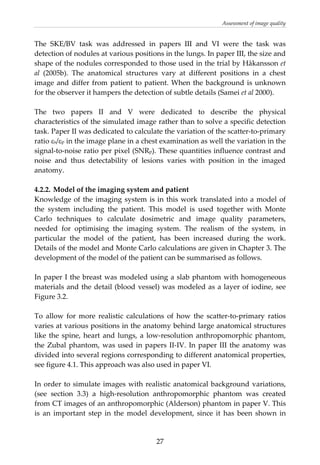
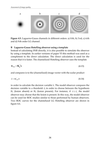

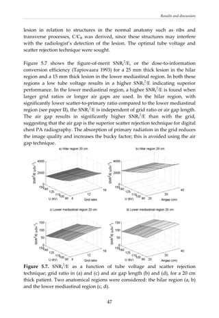
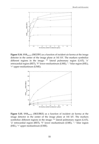


This document provides a summary of a dissertation titled "Quantifying image quality in diagnostic radiology using simulation of the imaging system and model observers" by Gustaf Ullman. The dissertation develops methods for assessing image quality in simulations of projection radiography using Monte Carlo modeling of the entire x-ray imaging system, from x-ray tube and patient to image detector and observer. Image quality is quantified by measures such as signal-to-noise ratio of lesions using model observers that mimic human observers. The methods are applied to chest and breast imaging to investigate optimal acquisition parameters for detecting lung lesions while minimizing patient dose.


![Licenza edilizia in sanatoria 2009 gambino giovanni c.e.s. n.11 2009[1]](https://cdn.slidesharecdn.com/ss_thumbnails/licenzaediliziainsanatoria2009gambinogiovannic-e-s-n-11-20091-121003040522-phpapp01-thumbnail.jpg?width=640&height=640&fit=bounds)


![PERI-PROSTHETIC FRACTURE NAIL-PLATE CONSTRUCT [NPC].pptx](https://cdn.slidesharecdn.com/ss_thumbnails/drarunkumardrmohamedashrafperiprostheticfrasturenail-plateconstructnpc-260209164459-7e9d15a1-thumbnail.jpg?width=640&height=640&fit=bounds)


![ONFH[AVN HIP] -TRIPLE REGIME -A NOVAL SURGICAL CONCEPT .pptx](https://cdn.slidesharecdn.com/ss_thumbnails/onfhavnhip2026koaconcalicutdrgokuldevdrmashraf-260210064517-213ec005-thumbnail.jpg?width=640&height=640&fit=bounds)


