Download as PDF, PPTX


![M. Bianchetti - Prudent Valuation – Global Derivatives – Budapest, 10 May 2016 p. 2
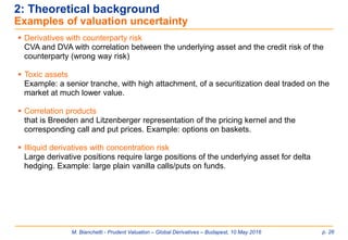
Summary [1]
1. Introduction
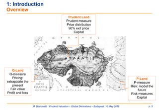
o Overview
o Prudent valuation history
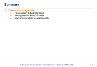
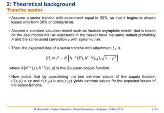
2. Theoretical Background
o Price opacity & financial crisis
o Pricing beyond Black-Scholes
o Market incompleteness & illiquidity
3. Regulation
o Overview
o The Capital Requirement Regulation 575/2013
o The EBA Regulatory Technical Standards
o AVAs vs XVAs
o Prudent valuation reporting
o Prudent valuation data NEW
NEW](https://image.slidesharecdn.com/prudentvaluation-long-v1-160602205124/85/Prudent-Valuation-2-320.jpg)
![M. Bianchetti - Prudent Valuation – Global Derivatives – Budapest, 10 May 2016 p. 3
Summary [2]
4. AVA calculation
o Definitions and basic assumptions
o Market price uncertainty AVA
o Close-out costs AVA
o Model risk AVA
o Unearned credit spreads AVA
o Investing and funding costs AVA
o Concentrated positions AVA
o Future administrative costs AVA
o Early termination AVA
o Operational risk AVA
5. Prudent valuation framework
o Implementation
o Methodological framework
o Operational framework
o IT framework
o Documentation & reporting
o Example of prudent valuation framework
6. Conclusions
7. References
8. Glossary
NEW](https://image.slidesharecdn.com/prudentvaluation-long-v1-160602205124/85/Prudent-Valuation-3-320.jpg)

![M. Bianchetti - Prudent Valuation – Global Derivatives – Budapest, 10 May 2016 p. 7
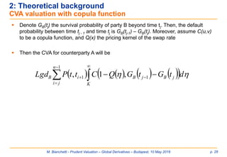
The idea of prudent valuation dates back to Basel 2 regulation (see BCBS,
“International Convergence of Capital Measurement and Capital Standards – A revised
framework”, June 2004).
In particular, sec. VI (“Trading book issues”), ch. B (“Prudent valuation guidance”), par.
690-701 set the requirements for prudent valuation in terms of
o systems and controls,
o valuation methodologies,
o valuation adjustments or reserves, impacting regulatory capital (not P&L).
The CRR inherited most of the contents in its art. 105.
In more recent times, prudent valuation has been required by the Financial Stability
Agency (FSA) to UK institutions, see refs. below.
o Financial Services Authority, “Dear CEO Letter: Valuation and Product Control”, August 2008,
http://www.fsa.gov.uk/pubs/ceo/valuation.pdf
o Financial Services Authority, “Product Control Findings and Prudent Valuation Presentation”, November 2010,
http://www.fsa.gov.uk/pubs/other/pcfindings.pdf
o Financial Services Authority, “Regulatory Prudent Valuation Return”, Policy Statement 12/7, April 2012,
http://www.fsa.gov.uk/library/policy/policy/2012/12-07.shtml
1: Introduction
Prudent valuation history [1/3]](https://image.slidesharecdn.com/prudentvaluation-long-v1-160602205124/85/Prudent-Valuation-7-320.jpg)
![M. Bianchetti - Prudent Valuation – Global Derivatives – Budapest, 10 May 2016 p. 8
1: Introduction
Prudent valuation history [2/3]
August 2008
FSA “Dear
CEO letter”
November 2010
FSA “Product Control
Findings and Prudent
Valuation Presentation”
April 2012
FSA “Regulatory Prudent
Valuation Return”, Policy
Statement
2008 2009 2010 2011 20122006 20072004 2005
June 2004
BCBS “International Convergence
of Capital Measurement and
Capital Standards” (Basel 2)](https://image.slidesharecdn.com/prudentvaluation-long-v1-160602205124/85/Prudent-Valuation-8-320.jpg)
![M. Bianchetti - Prudent Valuation – Global Derivatives – Budapest, 10 May 2016 p. 9
1: Introduction
Prudent valuation history [3/3]
13 November 2012
EBA Discussion
Paper
(EBA/DP/2012/03)
10 July 2013
EBA Consultation
Paper
(EBA/CP/2013/28)
1 Jan. 2014
CRR
575/2013
31 March 2014
EBA Final Draft RTS
and first application of
prudent valuation
28 Jan. 2016
EBA RTS
published on
OJEU
8 November 2013
EBA Quantitative
Impact Study
2012 2013 2014 2015
23 Jan. 2015
EBA Final Draft
RTS amended
Prudent valuation in
place
2016
28 October 2015
EU commission
adoption of EBA RTS
NEW](https://image.slidesharecdn.com/prudentvaluation-long-v1-160602205124/85/Prudent-Valuation-9-320.jpg)
![M. Bianchetti - Prudent Valuation – Global Derivatives – Budapest, 10 May 2016 p. 16
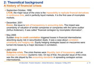
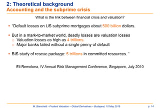
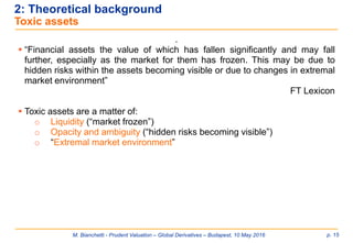
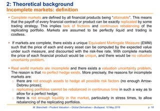
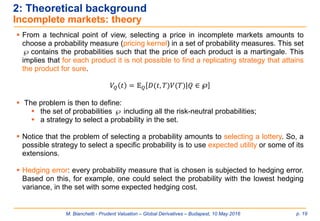
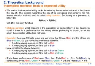
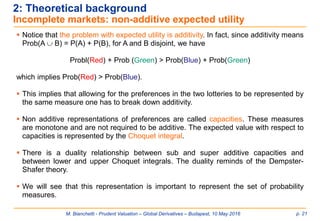
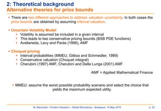
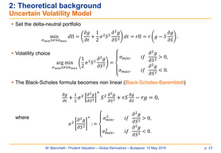
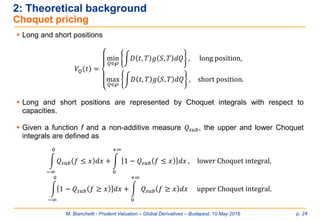
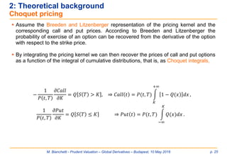
2: Theoretical background
A simple example [1]
Take a very simple financial product, that is an equity linked note promising to pay a
participation to the increase in some stock market index in five years.
The replicating portfolio of the product is made up by:
o A zero coupon bond paying the Libor with five years maturity
o A zero coupon bond paying the credit risk spread of the issuer with five years
maturity
o An equity option with five years exercise time
The main sources of valuation uncertainty are the following.
o The calibration of the five year zero coupon Libor, using fixed income market
data and bootstrapping techniques. This valuation problem is common to other
fixed income products.
o The calibration of the five year zero coupon credit spread, using the issuer’s or
comparable CDS and bond data, and bootstrapping techniques.
o The calibration of the five year equity volatility, using equity options’ market data
and bootstrapping techniques. Typically, exchange traded or OTC derivatives do
not have a liquid market for 5 years maturity and we must extend implied
volatility beyond the traded maturities.](https://image.slidesharecdn.com/prudentvaluation-long-v1-160602205124/85/Prudent-Valuation-16-320.jpg)
![M. Bianchetti - Prudent Valuation – Global Derivatives – Budapest, 10 May 2016 p. 17
2: Theoretical background
A simple example [2]
There are actually other risk sources, mostly the correlations among the risk factors
involved.
o Correlation between equity and bonds
It could seem that this should not affect the pricing problem, since it is made under
the Forward Martingale Measure (FMM), but the volatility of the forward price
depends on correlation.
o Correlation between underlying asset and volatility
This is relevant in cases in which the underlying asset and its volatility co-move in
directions leading to a decrease of the embedded option. This is not the case of
this product, which is long both in the underlying asset and its volatility, while the
equity market and volatility are known to be negatively correlated.
o Correlation between the embedded option and the credit quality of the issuer
Actually the embedded option is a vulnerable option whose value is affected by the
positive correlation between the exposure (the exercise of the option) and the
default probability of the issuer.](https://image.slidesharecdn.com/prudentvaluation-long-v1-160602205124/85/Prudent-Valuation-17-320.jpg)
![M. Bianchetti - Prudent Valuation – Global Derivatives – Budapest, 10 May 2016 p. 29
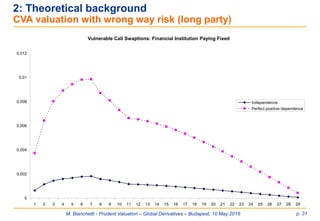
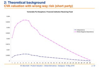
2: Theoretical background
CVA valuation with wrong way risk
Now assume perfect dependence between the underlying asset and default of the
counterparty. In this case, we have the Fréchet bound 𝒞 𝑥, 𝑦 ≤ 𝑀𝑖𝑛 𝑥; 𝑦 .
In this case, the CVA can be computed in closed form as
CVA = LgdBmax[k*(tj) – k,0]A(t, tj, tn) [GB(tj-1) – GB(tj)]
– LgdB PayerSwaption(.;max(k*(tj),k))
where k*(tj) is defined from Q((sr(tj,tn) > k*(tj)) = GB(tj-1) – GB(tj), and
is the swap annuity.
𝐴(𝑡; 𝑡𝑗, 𝑡 𝑛) =
𝑖=𝑗
𝑛−1
𝑃 𝑡, 𝑡𝑖−1 𝜏𝑖](https://image.slidesharecdn.com/prudentvaluation-long-v1-160602205124/85/Prudent-Valuation-29-320.jpg)
![M. Bianchetti - Prudent Valuation – Global Derivatives – Budapest, 10 May 2016 p. 30
2: Theoretical background
CVA valuation with wrong way risk
o For the short end of the contract the worst scenario is perfect negative dependence
between the underlying asset and default of the counter party. In this case, we have
the Fréchet bound 𝒞 𝑥, 𝑦 > 𝑀𝑖𝑛 𝑥 + 𝑦 − 1; 0 .
In this case, the CVA can be computed in closed form as
CVA = LgdA[ReceiverSwaption(.;min(k*(tj),k)) – Receiver swaption(.;k)]
+ LGDA max[k – k*(tj),0](1 – GA(tj – 1) – GA(tj))](https://image.slidesharecdn.com/prudentvaluation-long-v1-160602205124/85/Prudent-Valuation-30-320.jpg)
![M. Bianchetti - Prudent Valuation – Global Derivatives – Budapest, 10 May 2016 p. 35
2: Theoretical background
Rainbow options
Assume a call option on the minimum of a set of assets (Everest). This can be priced
with a Choquet integral using the copula as the Choquet integral
From the point of view of the issuer, we can compute the conservative value in closed
form, for a bivariate product
dTSQTSQTSQCTtP
TKSSSCall
K
N
N
))((),...)((),)((,
),),,...,(min(
21
21
)*,max(;,
;,*;,
,,
2
11*
*],max[
2
*
11* 2
KKtSC
KtSCKtSC
dSQTtPdSQTtPC
KK
KK
K
K
KK
1
1 ](https://image.slidesharecdn.com/prudentvaluation-long-v1-160602205124/85/Prudent-Valuation-35-320.jpg)
![M. Bianchetti - Prudent Valuation – Global Derivatives – Budapest, 10 May 2016 p. 39
Market
Data
Models
Estim
ates
Fair Value
accounting AVA
(Additional
Valuation
Adjustment)
IFRS 13
Prudent valuation
Prudent value
Deducted from Common
Equity Tier 1 capital
CRR article 105 requisites
Policies &
procedures
Control
systems
Prudent
valuation
principles
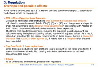
3: Regulation
CRR 575/2013 [1/8]](https://image.slidesharecdn.com/prudentvaluation-long-v1-160602205124/85/Prudent-Valuation-39-320.jpg)
![M. Bianchetti - Prudent Valuation – Global Derivatives – Budapest, 10 May 2016 p. 40
3: Regulation
CRR 575/2013 [2/8]
Art. 34
Prudent valuation
scope
Systems and
controls
Valuation
Valuation
adjustments
Art. 105
CRR
575/2013
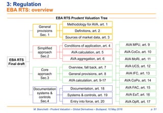
CRR Prudent Valuation Tree
Prudent valuation
principles
Degree of certainty, art. 105.1
S&C requirements, art. 105.2
Revaluation frequency art. 105.3
Mark to market, art. 105.4-5
Mark to model, art. 105.6-7
IPV, art. 105.8
Valuation adjustments, art. 105.9-10
Illiquid positions, art. 105.11
Other valuation adj., art. 105.12
Complex products, art. 105.13](https://image.slidesharecdn.com/prudentvaluation-long-v1-160602205124/85/Prudent-Valuation-40-320.jpg)
![M. Bianchetti - Prudent Valuation – Global Derivatives – Budapest, 10 May 2016 p. 41
CRR art. 34: scope and target
o Scope: all assets measured at fair value
o Target: CET1 capital (not P&L)
3: Regulation
CRR 575/2013 [3/8]](https://image.slidesharecdn.com/prudentvaluation-long-v1-160602205124/85/Prudent-Valuation-41-320.jpg)
![M. Bianchetti - Prudent Valuation – Global Derivatives – Budapest, 10 May 2016 p. 42
CRR art. 105.1, scope and degree of certainty: all positions are subject to prudent
valuation, achieving an appropriate degree of certainty with regard to:
o the dynamic nature of the positions,
o the demands of prudential soundness, and
o the mode of operation and purpose of capital requirements in respect of trading book
positions.
CRR art 105.2, systems and controls: institutions establish and maintain systems and
controls to ensure prudent and reliable valuations, including at least.
o Documented policies and procedures for the valuation process, including:
• clearly defined responsibilities of the various areas involved in the determination of the
valuation,
• sources of market information and review of their reliability,
• guidelines for the use of unobservable inputs that reflect the assumptions of authority on
the elements used by market participants to determine the price of the position,
• frequency of independent valuation,
• timing of closing prices,
• procedures for the correction of assessments,
• procedures for the reconciliation of month end and ad hoc.
o Clear and independent (of the front office) reporting lines for the department in charge of the
valuation process.
3: Regulation
CRR 575/2013 [4/8]](https://image.slidesharecdn.com/prudentvaluation-long-v1-160602205124/85/Prudent-Valuation-42-320.jpg)
![M. Bianchetti - Prudent Valuation – Global Derivatives – Budapest, 10 May 2016 p. 43
CRR art 105.3, revaluation frequency: institutions revalue trading book positions at
least daily
CRR art 105.4-5, mark to market: institutions mark their positions to market whenever
possible, using the more prudent side of bid and offer unless they can close out at mid
market.
CRR art 105.6, mark to model: where marking to market is not possible, institutions
must conservatively mark to model their positions and portfolios.
3: Regulation
CRR 575/2013 [5/8]](https://image.slidesharecdn.com/prudentvaluation-long-v1-160602205124/85/Prudent-Valuation-43-320.jpg)
![M. Bianchetti - Prudent Valuation – Global Derivatives – Budapest, 10 May 2016 p. 44
CRR art 105.7, mark to model:
o senior management must be aware of the fair-valued positions marked to model and must
understand the materiality of the uncertainty of the risk/performance of the business;
o source market inputs, where possible, in line with market prices, and assess the
appropriateness of market inputs and model parameters on a frequent basis;
o use valuation methodologies which are accepted market practice;
o where the model is developed by the institution itself, it must be based on appropriate
assumptions, assessed and challenged by suitably qualified parties independent of the
development process;
o have in place formal change control procedures, hold a secure copy of the model and use
it periodically to check valuations;
o risk management must be aware of the weaknesses of the models used and how best to
reflect those in the valuation output;
o models are subject to periodic review to determine the accuracy of their performance,
including assessment of the continued appropriateness of assumptions, analysis of profit
and loss versus risk factors, and comparison of actual close out values to model outputs;
o the model must be developed or approved independently
of the trading desk and independently tested, including
validation of the mathematics, assumptions and software
implementation.
3: Regulation
CRR 575/2013 [6/8]
Very detailed article
regarding valuation
in general](https://image.slidesharecdn.com/prudentvaluation-long-v1-160602205124/85/Prudent-Valuation-44-320.jpg)
![M. Bianchetti - Prudent Valuation – Global Derivatives – Budapest, 10 May 2016 p. 45
CRR art. 105.8, independent price verification (IPV): institutions perform independent
price verification in addition to daily marking to market/model. Verification of market
prices and model inputs must be performed by unit independent from units that benefit
from the trading book, at least monthly, or more frequently depending on the nature of
the market or trading activity. Where independent pricing sources are not available or
pricing sources are more subjective, prudent measures such as valuation adjustments
may be appropriate.
CRR art 105.9-10: valuation adjustments: institutions establish and maintain
procedures for considering valuation adjustments, and formally consider the following:
unearned credit spreads, close-out costs, operational risks, market price uncertainty,
early termination, investing and funding costs, future administrative costs and, where
relevant, model risk.
CRR art 105.11, illiquid/concentrated positions: Institutions shall establish and
maintain procedures for calculating an adjustment to the current valuation of any less
liquid positions, which can in particular arise from market events or institution-related
situations such as concentrated positions and/or positions for which the originally
intended holding period has been exceeded.
3: Regulation
CRR 575/2013 [7/8]](https://image.slidesharecdn.com/prudentvaluation-long-v1-160602205124/85/Prudent-Valuation-45-320.jpg)
![M. Bianchetti - Prudent Valuation – Global Derivatives – Budapest, 10 May 2016 p. 46
CRR art. 105.12, other valuation adjustments:
institutions must consider whether to apply a valuation adjustment also:
o when using third party valuations,
o when marking to model,
o for less liquid positions, including an ongoing basis review their continued suitability,
o for uncertainty of parameter inputs used by models.
CRR art. 105.13, complex products: institutions must explicitly assess the need for
valuation adjustments to reflect the model risk associated with using:
o a possibly incorrect valuation methodology
o unobservable (and possibly incorrect) calibration parameters in the valuation model.
3: Regulation
CRR 575/2013 [8/8]](https://image.slidesharecdn.com/prudentvaluation-long-v1-160602205124/85/Prudent-Valuation-46-320.jpg)
![M. Bianchetti - Prudent Valuation – Global Derivatives – Budapest, 10 May 2016 p. 47
3: Regulation
Fair Value Vs Prudent Value [1]
Fair Value
o Regulation: IFRS13
o Application: balance sheet
o Percentile: 50% (expected
value)
o The price that would be received
to sell an asset or paid to
transfer a liability in an orderly
transaction between market
participants at the measurement
date
o Must include all the factors that
a market participants would use,
acting in their economic best
interest.
o Atoms: single trades.
o Fair value adjustments
o Non-entity specific
Prudent value
o Regulation: CRR/EBA
o Application: CET1
o Percentile: 90%
o Must reflect the exit price at which
the institution can trade within the
capital calculation time horizon.
o Atoms: valuation positions subject
to a specific source of price
unertainty
o Entity specific
o Subject to diversification benefit
(50% weight for MPU, CoCo, MoRi
AVAs)](https://image.slidesharecdn.com/prudentvaluation-long-v1-160602205124/85/Prudent-Valuation-47-320.jpg)
![M. Bianchetti - Prudent Valuation – Global Derivatives – Budapest, 10 May 2016 p. 48
3: Regulation
Fair Value Vs Prudent Value [2]
Why capital and not P&L ?
P&L is accounted under accounting standards
o EU listed companies: use IFRS (International Financial Reporting Standards),
established and maintained by the IASB (International Accounting Standards
Board) see www.ifrs.org
o US listed companies: use GAAP (Generally Accepted Accounting Standards),
established and maintained by the FASB (Financial Accounting Standards Board),
see www.fasb.org
o Convergence towards IFRS is in progress
Both IFRS and GAAP define the fair value as an exit price, not as a prudent price. Fair
value must be fair, not prudent.
Thus, regulators have decided to account for prudent price through capital, instead of
altering the accounting standards.](https://image.slidesharecdn.com/prudentvaluation-long-v1-160602205124/85/Prudent-Valuation-48-320.jpg)
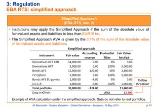
![M. Bianchetti - Prudent Valuation – Global Derivatives – Budapest, 10 May 2016 p. 52
3: Regulation
EBA RTS: prudent valuation scope [1/9]
General rules
Region of application: since the CRR is an EU directive, prudent valuation applies to
all institutions within EU countries. In case of institution made of a central holding and
one or more subsidiaries, prudent valuation applies to those individual subsidiaries
included in EU countries.
Scope of application: the CRR art. 5, defines the prudent valuation scope as including
all trading book positions. However, the CRR art. 34 requires that institutions apply the
standards of art. 105 to all assets measured at fair value. The combination of the above
CRR articles 34 and 105 implies that the prudent valuation scope includes all fair-valued
positions, regardless of whether they are held in the trading book or banking book.
The positions at fair value held in both trading and banking books are the following:
Assets Liabilities
Financial assets held for trading (HFT) Financial liabilities held for trading (HFT)
Financial assets at fair value Financial liabilities at fair value
Financial assets available for sale (AFS) (for
the portion not subject to prudential filters)](https://image.slidesharecdn.com/prudentvaluation-long-v1-160602205124/85/Prudent-Valuation-52-320.jpg)
![M. Bianchetti - Prudent Valuation – Global Derivatives – Budapest, 10 May 2016 p. 53
3: Regulation
EBA RTS: prudent valuation scope [2/9]
Positions excluded:
o the EBA RTS, art. 4.2 and 8.1, allow Institutions to exclude partially or totally from the
prudent valuation scope those positions for which a change in their accounting fair
value has only a partial or zero impact on Common Equity Tier 1 capital. These
positions must be included in proportion to the impact of the relevant valuation
change on CET1 capital.
o In particular these positions are the following:
1. positions subject to prudential filters,
2. exactly matching, offsetting positions (back to back),
3. positions in hedge accounting.
o Notice that, since the size of the positions above may be relevant, the prudent
valuation scope is the primary driver of the AVA figures.
o How to compute inclusion/exclusion in practice ? See next slides.](https://image.slidesharecdn.com/prudentvaluation-long-v1-160602205124/85/Prudent-Valuation-53-320.jpg)
![M. Bianchetti - Prudent Valuation – Global Derivatives – Budapest, 10 May 2016 p. 54
3: Regulation
EBA RTS: prudent valuation scope [3/9]
1. Positions subject to prudential filers
o Positions subject to prudential filters refer to the "Financial assets available for sale"
(AFS). The inclusion/exclusion of these positions from the prudent valuation scope
of application follows the CRR requirements.
o The exact percentages of partial inclusions follows the transitional provisions that
each local Regulator issued in compliance with the above CRR requirements.
o Partial inclusion means, for instance, that if 40% of fair value gains and losses are
filtered in CET1, the residual 60% of fair value gains and losses are included in the
prudent valuation scope. In case of 100% filter, the position is completely excluded
by prudent valuation.
Position under prudential filters (AFS) Inclusion
Government bonds issued by EU countries 0%
Other debt securities (excluding the EU
government bonds above)
Partial inclusion depending on the sign of
the reserve and on local prescriptions
Equity
Partial inclusion depending on the sign of
the reserve and on local prescriptions](https://image.slidesharecdn.com/prudentvaluation-long-v1-160602205124/85/Prudent-Valuation-54-320.jpg)
![M. Bianchetti - Prudent Valuation – Global Derivatives – Budapest, 10 May 2016 p. 55
Transitional provisions issued by national regulators.
3: Regulation
EBA RTS: prudent valuation scope [4/9]
Circolare 285 Banca d’Italia
The applicable percentage following art. 467, par. 3 CRR is:
a) 20% since 1 Jan. 2014 to 31 Dec. 2014
b) 40% since 1 Jan. 2015 to 31 Dec. 2015
c) 60% since 1 Jan. 2016 to 31 Dec. 2016
d) 80% since 1 Jan. 2017 to 31 Dec. 2017
Local
regulation
in Italy
Article 467 CRR
[…] institutions shall include in the calculation of their Common
Equity Tier 1 items only the applicable percentage](https://image.slidesharecdn.com/prudentvaluation-long-v1-160602205124/85/Prudent-Valuation-55-320.jpg)
![M. Bianchetti - Prudent Valuation – Global Derivatives – Budapest, 10 May 2016 p. 56
3: Regulation
EBA RTS: prudent valuation scope [5/9]
Institutions may not include in own funds unrealized gains and losses related to AFS
positions with central administrations.
Circolare 285 Banca d’Italia
The applicable percentage following art. 468, par. 3 CRR is:
a) 100% 1 Jan. 2014 to 31 Dec. 2014
b) 60% since 1 Jan. 2015 to 31 Dec. 2015
c) 40% since 1 Jan. 2016 to 31 Dec. 2016
d) 20% since 1 Jan. 2017 to 31 Dec. 2017
Article 468 CRR
[…] institutions shall remove in the calculation of their Common
Equity Tier 1 items only the applicable percentage
Local
regulation
in Italy](https://image.slidesharecdn.com/prudentvaluation-long-v1-160602205124/85/Prudent-Valuation-56-320.jpg)
![M. Bianchetti - Prudent Valuation – Global Derivatives – Budapest, 10 May 2016 p. 57
3: Regulation
EBA RTS: prudent valuation scope [6/9]
According to Regulation (EU) 2016/445 of the European Central Bank of 14 Mar 2016
(published OJEU on 26 Mar. 2016), art. 14 and 15, the corresponding art. 467 and 468
of CRR (setting prudential filters for AFS positions) are modified such that AFS positions
in EU government Bonds shall no longer subject to 100% filter, but shall be subject to
standard prudential filters holding for other AFS position:
Inclusion of unrealized losses (art. 14 -> art. 467 CRR):
o 60% in [1/1/2016 – 31/12/2016]
o 80% in [1/1/2017 – 31/12/2017]
Exclusion of unrealized gains (art. 15 -> art. 468 CRR):
o 40% in [1/1/2016 – 31/12/2016]
o 20% in [1/1/2017 – 31/12/2017]
First application date: Q4-2016
This regulatory change will change substantially the AVA figures for institutions
with huge positions in EU govies (more or less all banks...).
NEW](https://image.slidesharecdn.com/prudentvaluation-long-v1-160602205124/85/Prudent-Valuation-57-320.jpg)
![M. Bianchetti - Prudent Valuation – Global Derivatives – Budapest, 10 May 2016 p. 58
3: Regulation
EBA RTS: prudent valuation scope [7/9]
2. Exactly matching, offsetting positions (back to back)
o Back to back positions are groups of trades with total null valuation exposure to
market risk factors (interest rates, volatility, etc.), since any variation in the relevant
market valuation inputs generates opposite variations in the value of the trades in
the group, such that the total value is constant. In other words, the group has null
total sensitivity to market risk factors.
o We stress that back to back positions are neutral w.r.t. other risk factors, such as
counterparty defaults, since the trades into the group may be subscribed with
different counterparties.
o From a prudent valuation point of view:
• Simplified approach: 100% exclusion (EBA RTS art. 4.2)
• Core approach: AVAs must be calculated based on the proportion of the
accounting valuation change that impacts CET1 capital (EBA RTS art. 8.1). In
practice:
• AVA MPU, CoCo and MoRi are null,
• AVA UCS, IFC, CoPo, FAC, EaT, OpR must be computed on the total
valuation exposure of the back to back portfolio.](https://image.slidesharecdn.com/prudentvaluation-long-v1-160602205124/85/Prudent-Valuation-58-320.jpg)
![M. Bianchetti - Prudent Valuation – Global Derivatives – Budapest, 10 May 2016 p. 59
3: Regulation
EBA RTS: prudent valuation scope [8/9]
3. Hedge accounting positions
o Hedge accounting positions are characterized by a hedged instrument (e.g. one ore
more securities, loans or mortgages, etc.) and an hedging instrument (e.g. one ore
more interest rate swaps, credit default swaps, etc.).
o The total package of hedged + hedging instruments has, by construction, a reduced
sensitivity to the underlying risk factors.
o From a prudent valuation point of view, all AVAs must be computed on the total
valuation exposure of the hedge accounting portfolio.](https://image.slidesharecdn.com/prudentvaluation-long-v1-160602205124/85/Prudent-Valuation-59-320.jpg)
![M. Bianchetti - Prudent Valuation – Global Derivatives – Budapest, 10 May 2016 p. 60
3: Regulation
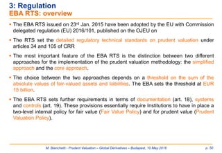
EBA RTS: prudent valuation scope [9/9]
Positions subject
to prudential
filters (AFS)
Positions in
hedge
accounting
Positions for which a
change in their
accounting fair value
has only a partial or
zero impact on CET 1
Art. 4.2 and 8.1
EBA RTS Prudent Valuation scope: exclusions
Positions in
back to back
EU Gov. bonds
Other bonds
Equity
General criteria
for exclusion
Positions excluded
% of
exclusion
100% until Sept. 16
Partial, phase in
Partial, phase in
Simplified appr.
Partial, residual exposure
of hedged + hedging items
Core appr.
100%
Partial, residual exposure
to UCS, IFC, CoPo, FAC,
EaT, OpR AVAs](https://image.slidesharecdn.com/prudentvaluation-long-v1-160602205124/85/Prudent-Valuation-60-320.jpg)
![M. Bianchetti - Prudent Valuation – Global Derivatives – Budapest, 10 May 2016 p. 62
3: Regulation
EBA RTS: core approach [1/3]
Core Approach (EBA RTS, sec. 3)
Institutions that at individual or consolidated level exceed the EUR15bn threshold must
apply the core approach.
Each AVA is the excess of valuation adjustments required to achieve the identified
prudent value, over any adjustment applied in the institution’s fair value that can be
identified as addressing the same source of valuation uncertainty as the AVA.
Whenever possible, the prudent value of a position is linked to the 90% percentile of its
price distribution. In practice for AVAs i) Market price uncertainty ii) Close-out costs iii)
Unearned credit spreads, the Institutions must compute the prudent value using the
available market data and the 90% target confidence.
Whenever insufficient data exists to construct a plausible range of values, institutions
shall use an expert-based approach using qualitative and quantitative information
available to achieve a 90% level of certainty in the prudent value.
Additional Valuation
Adjustments](https://image.slidesharecdn.com/prudentvaluation-long-v1-160602205124/85/Prudent-Valuation-62-320.jpg)
![M. Bianchetti - Prudent Valuation – Global Derivatives – Budapest, 10 May 2016 p. 63
3: Regulation
EBA RTS: core approach [2/3]
Core approach
Additional Valuation Adjustments
Market
Price
Uncertainty
(MPU)
Art. 9
Close Out
Costs
(CoCo)
Art. 10
Model Risk
(MoRi)
Art. 11
Unearned
Credit
Spread
(UCS)
Art. 12
Investing &
Funding
Cost
(IFC)
Art. 13
Concen-
trated
Positions
(CoPo)
Art. 14
Future
Admin
Costs
(FAC)
Art. 15
Early
Termination
(EaT)
Art. 16
Main
AVAs
UCS/IFC
AVAs
Other
AVAs
Operational
Risk
(OpR)
Art. 17
The AVA hierarchy
Market risk factors
50% weights for diversification
Market risk factors
Split onto main AVAs
Non-market risk factors
100% weights, no diversification](https://image.slidesharecdn.com/prudentvaluation-long-v1-160602205124/85/Prudent-Valuation-63-320.jpg)
![M. Bianchetti - Prudent Valuation – Global Derivatives – Budapest, 10 May 2016 p. 64
3: Regulation
EBA RTS: core approach [3/3]
Example of AVA calculation and aggregation
under the core approach.
IFC and UCS AVAs are split into their MPU, CoCo and
MoRi components and pre-aggregated to the
corresponding AVAs, then the total AVA is obtained from
the aggregation of the other seven residual AVAs. In order
to show toy but realistic figures, we assumed the principal
AVAs equal to 1/7 of the 99% x 0.1% of the total FV under
the core approach. AVA OpR has been calculated as for a
non-AMA Institution. In the last line, we also add a
possible AVA fall-back calculated on the remaining 1% x
0.1% of the total FV.
Above
threshold](https://image.slidesharecdn.com/prudentvaluation-long-v1-160602205124/85/Prudent-Valuation-64-320.jpg)
![M. Bianchetti - Prudent Valuation – Global Derivatives – Budapest, 10 May 2016 p. 65
3: Regulation
EBA RTS: fall-back approach [1/2]
Fall back approach (EBA RTS, art. 7.2.b)
Institutions that exceed the EUR15bn threshold but cannot calculate the core approach
AVAs for certain positions, are allowed to apply a «fall-back approach» (actualy very
capital intensive), and compute AVAs for those positions as the sum of:
100% of the net unrealised profit (NUP)
10% of the notional value in case of derivatives;
25% of the absolute difference between the fair value (FV) and the net unrealised
profit for non-derivatives.
In formulas:
"unrealised profit shall mean the change, where positive, in fair value since trade
inception, determined on a first-in-first-out basis.”
A𝑉𝐴 𝑓𝑏 = 100% 𝑁𝑈𝑃+
+ 10% 𝑁 𝐷𝑒𝑟 + 25% 𝐹𝑉 − 𝑁𝑈𝑃+
𝑁𝑜𝑛−𝐷𝑒𝑟
𝑁𝑈𝑃+
: = 𝑚𝑎𝑥
𝑖=1
𝑁 𝑓𝑏
𝑁𝑈𝑃𝑖 , 0 , 𝑁 𝐷𝑒𝑟 =
𝑖=1
𝑁 𝑓𝑏
𝑁𝑖 , 𝐹𝑉 =
𝑖=1
𝑁 𝑓𝑏
𝐹𝑉𝑖 .](https://image.slidesharecdn.com/prudentvaluation-long-v1-160602205124/85/Prudent-Valuation-65-320.jpg)
![M. Bianchetti - Prudent Valuation – Global Derivatives – Budapest, 10 May 2016 p. 66
3: Regulation
EBA RTS: fall-back approach [2/2]
Example of AVA
calculation under the
fall-back approach. We
assume to apply the
Fall-Back approach to
the 1% portion of the
previous core portfolio.
The net unrealized
P&Ls are the 0.1% of
the fair values, positive
for derivatives and
negative for bonds. The
notional for derivatives
is assumed 10 times
the fair value. The AVA
Fall-Back is then
summed to the
remaining 99% of the
previous AVA core to
obtain the total AVA.](https://image.slidesharecdn.com/prudentvaluation-long-v1-160602205124/85/Prudent-Valuation-66-320.jpg)
![M. Bianchetti - Prudent Valuation – Global Derivatives – Budapest, 10 May 2016 p. 67
The core approach is mandatory only for institutions above the threshold of €15 bln.
Institutions below the threshold may choose between simplified and core approaches.
Which one is more convenient (generate smaller capital absorption) ?
There is no precise mathematical relation between the simplified and core AVAs.
The actual figures depend principally on the actual positions
included in the prudent valuation scope.
3: Regulation
Simplified vs core approaches [1/2]](https://image.slidesharecdn.com/prudentvaluation-long-v1-160602205124/85/Prudent-Valuation-67-320.jpg)
![M. Bianchetti - Prudent Valuation – Global Derivatives – Budapest, 10 May 2016 p. 70
Recently, two regulators proposed a consultation on enhancements to the reporting of
prudent valuation figures.
The industry (ISDA, IIF, AFME, etc.) is actively discussing the proposed template and
comments to BCBS are expected. Main issues are the following:
o Partial overlapping and consistency of AVA definitions under BCBS and EBA RTS
o Different AVA scopes of applications, since EBA RTS allows for many exclusions.
o AVAs break down by asset class is problematic for EU Institutions because EBA RTS
requires AVA calculation at valuation exposure level. For example, AVA MPU for some
risk factor (e.g. IR/vols and FX rates/vols) naturally include multiple asset classes.
1. BCBS Consultative Document, “Pillar 3 disclosure requirements –
consolidated and enhanced framework”, March 2016, issued for
comment by 10 June 2016.
Template PV1, in particular, aims to disclose prudent valuation
figures under Pillar 3, consistently with previous BCBS
requirements:
o BCBS “International Convergence of Capital Measurement and
Capital Standards” (Basel 2, comprehensive version) June 2006,
paragraphs 698-701.
o BCBS “Supervisory guidance for assessing banks’ financial
instrument fair value practices”, April 2009 (in particular Principle
10).
3: Regulation
Prudent valuation reporting [1/3]
NEW](https://image.slidesharecdn.com/prudentvaluation-long-v1-160602205124/85/Prudent-Valuation-70-320.jpg)
![M. Bianchetti - Prudent Valuation – Global Derivatives – Budapest, 10 May 2016 p. 71
Template PV1 proposed in BCBS Consultative Document,
“Pillar 3 disclosure requirements – consolidated and enhanced framework”, March 2016, issued for comment by 10 June 2016.
3: Regulation
Prudent valuation reporting [2/3]
NEW](https://image.slidesharecdn.com/prudentvaluation-long-v1-160602205124/85/Prudent-Valuation-71-320.jpg)
![M. Bianchetti - Prudent Valuation – Global Derivatives – Budapest, 10 May 2016 p. 72
2. EBA consultation paper (EBA/CP/2016/02), ”Draft
implementing Technical Standards amending Commission
Implementing Regulation (EU) 680/2014 on supervisory
reporting of institutions”, 4 March 2016, issued for comment
by 31 March 2016.
The proposed amendement of prudent valuation
supervisory reporting is articulated into four new templates.
Template C 32.01: fair valued asset and liabilities
o Rows: accounting categorisation (HFT, AFS, etc.)
o Columns: fair value amounts of inclusions and
exclusions according to EBA RTS
Template C 32.02: core approach
o Rows: break down by portfolio/trade class (vanilla/exotic), diversification benefit, fall back app.
o Columns: AVAs and fair value adjustments according to EBA RTS.
Template C 32.03: focus on AVA MoRi
Template C 32.01: focus on AVA CoPo
Main issues are the following:
breakdown by portfolio/trade class (vanilla/exotic) is not consistent with AVA calculation by
valuation exposures,
amount of data required
3: Regulation
Prudent valuation reporting [3/3]
NEW](https://image.slidesharecdn.com/prudentvaluation-long-v1-160602205124/85/Prudent-Valuation-72-320.jpg)
![M. Bianchetti - Prudent Valuation – Global Derivatives – Budapest, 10 May 2016 p. 73
FV under prudent valuation scope = FV asset & liabilities – FV under prudential filters
3: Regulation
Prudent valuation data: QIS [1/3]](https://image.slidesharecdn.com/prudentvaluation-long-v1-160602205124/85/Prudent-Valuation-73-320.jpg)
![M. Bianchetti - Prudent Valuation – Global Derivatives – Budapest, 10 May 2016 p. 74
The EBA conducted a QIS to estimate the total impact of the requirements of the RTS
including 59 banks across 15 jurisdictions, with the following results.
Small banks: < 15 €/bln
Medium banks: 15 - 100 €/bln
Large banks: > 100 €/bln
Average
227 €/mln
per bank
3: Regulation
Prudent valuation data: QIS [2/3]](https://image.slidesharecdn.com/prudentvaluation-long-v1-160602205124/85/Prudent-Valuation-74-320.jpg)
![M. Bianchetti - Prudent Valuation – Global Derivatives – Budapest, 10 May 2016 p. 75
According to EBA: [*]
approximately 6,500 credit institutions across EEA Member States (as of 2013) report
supervisory data to their respective competent authorities.
Total value of assets: approximately EUR 42,000 billion.
Approximately 750 institutions (11%) are above the EUR 15 billion threshold.
[*] European Banking Authority, Consultation Paper, “Draft Implementing Technical Standards amending
Commission Implementing Regulation (EU) 680/2014 on supervisory reporting of institutions”, 4 March 2016,
https://www.eba.europa.eu/-/eba-seeks-comments-on-reporting-of-prudent-valuation-
information
3: Regulation
Prudent valuation data: QIS [3/3]](https://image.slidesharecdn.com/prudentvaluation-long-v1-160602205124/85/Prudent-Valuation-75-320.jpg)
![M. Bianchetti - Prudent Valuation – Global Derivatives – Budapest, 10 May 2016 p. 76
3: Regulation
Prudent valuation data: 2014-2015 [1/3]
Source: elaboration of public data (in collaboration with Ernst Young).
NEW](https://image.slidesharecdn.com/prudentvaluation-long-v1-160602205124/85/Prudent-Valuation-76-320.jpg)
![M. Bianchetti - Prudent Valuation – Global Derivatives – Budapest, 10 May 2016 p. 77
3: Regulation
Prudent valuation data: 2014-2015 [2/3]
Source: elaboration of public data (in collaboration with Ernst Young).
NEW](https://image.slidesharecdn.com/prudentvaluation-long-v1-160602205124/85/Prudent-Valuation-77-320.jpg)
![M. Bianchetti - Prudent Valuation – Global Derivatives – Budapest, 10 May 2016 p. 78
Comments
Fair value is given by FV assets + FV liablities including
o Held for trading (HFT)
o Fair Value Option (FVO)
o Hedging Derivatives (HD)
o Available For Sale (AFS)
Fair value for prudent valuation has been estimated from fair value excluding HD and
AFS (100%, no AFS filters applied, slightly underestimated).
AVA/CET1 figures are rather different, ranging from negligible to important %.
AVA core / AVA simplified > 1 in a few cases, thus AVA simplified is neither an AVA
cap nor an AVA floor.
Prudent valuation not driven by L3 instruments: moving from AVA/L3 to AVA /(L2+L3)
changes the figures by a factor of 100.
2014-2015 average AVAs double the 2013 QIS result (500 vs 227 mln€).
3: Regulation
Prudent valuation data: 2014-2015 [3/3]
NEW](https://image.slidesharecdn.com/prudentvaluation-long-v1-160602205124/85/Prudent-Valuation-78-320.jpg)
![M. Bianchetti - Prudent Valuation – Global Derivatives – Budapest, 10 May 2016 p. 79
1. XVAs
3: Regulation
Prudent valuation data: survey [1/4]
Restricted access to clients only
Dec.2015
30 respondents (18 GSIBs, 15 UK)
60 questions
EBA RTS not yet in place at the time
One third does not account FVA in fair
value, more than half does account AVA
IFC in prudent value.
MVA and KVA are not accounted both in
fair and prudent values.
NEW](https://image.slidesharecdn.com/prudentvaluation-long-v1-160602205124/85/Prudent-Valuation-79-320.jpg)
![M. Bianchetti - Prudent Valuation – Global Derivatives – Budapest, 10 May 2016 p. 80
1. XVAs (cont’d)
3: Regulation
Prudent valuation data: survey [2/4]
Only 30% use a spread term structure
«Peer estimate» is a possible answer to
the question «what is an exit price for
FVA ?»
Possible use of Markit XVA service
Both funding spreads sources and term
structures vary considerably, both for
FVA (Fair Value) and for AVA IFC
(prudent value)
NEW](https://image.slidesharecdn.com/prudentvaluation-long-v1-160602205124/85/Prudent-Valuation-80-320.jpg)
![M. Bianchetti - Prudent Valuation – Global Derivatives – Budapest, 10 May 2016 p. 81
2. P&L variance test
3: Regulation
Prudent valuation data: survey [3/4]
The P&L variance test is difficult to run
and pass in case of many relevant risk
factors, and may lead to huge AVA MPU.
60% ignore the P&Lvariance test
Only 7% run extensive application
Only 14% apply with quarterly frequency
NEW](https://image.slidesharecdn.com/prudentvaluation-long-v1-160602205124/85/Prudent-Valuation-81-320.jpg)
![M. Bianchetti - Prudent Valuation – Global Derivatives – Budapest, 10 May 2016 p. 82
3. Other
3: Regulation
Prudent valuation data: survey [4/4]
One half does apply/does not apply
offsetting between AVAs and other
regulatory capital reserves.
Possible offsets should be clarified, to
avoid possible capital double countings.
One third reduces the valuation
exposure.
NEW](https://image.slidesharecdn.com/prudentvaluation-long-v1-160602205124/85/Prudent-Valuation-82-320.jpg)
![M. Bianchetti - Prudent Valuation – Global Derivatives – Budapest, 10 May 2016 p. 84
4: AVA calculation
Definitions and basic assumptions [1]
In other words, a valuation position will display valuation exposures to its valuation
inputs. Clearly the degree of valuation exposure to a valuation input depends on the
particular valuation position.
Definitions (EBA RTS art. 2)
Item Definition Example
Valuation
position
A portfolio of financial instruments or
commodities measured at fair value, held in
both trading and non-trading books
E.g. a portfolio of
derivatives
Valuation
input
A set of parameters (observable or non-
observable) that influences the fair value of a
valuation position
E.g. yield curve,volatility
cube, market/historical
correlations, prepayment,
etc.
Valuation
exposure
The amount of a valuation position which is
sensitive to the change in a valuation input
E.g. the trades in portfolio
above sensible to the
valuation inputs above.](https://image.slidesharecdn.com/prudentvaluation-long-v1-160602205124/85/Prudent-Valuation-84-320.jpg)
![M. Bianchetti - Prudent Valuation – Global Derivatives – Budapest, 10 May 2016 p. 85
4: AVA calculation
Definitions and basic assumptions [2]
Fair value
In general, we denote the fair value of a valuation position 𝑝𝑖 at time t with 𝐹𝑉 𝑡, 𝑝𝑖 or,
shortly, with 𝐹𝑉𝑖 𝑡 , with 𝑖 = 1, … , 𝑁 𝑝. Given a set of valuation positions subject to
prudent valuation, we denote the total fair value as
𝐹𝑉 𝑡 =
𝑖=1
𝑁 𝑝
𝐹𝑉𝑖 𝑡
In the context of prudent valuation, we consider the following properties of fair value FV.
FV is positive for assets (𝐹𝑉𝑖 𝑡 > 0) and negative for liabilities (𝐹𝑉𝑖 𝑡 < 0).
Financial institutions have appropriate internal IPV process in place (EBA RTS, p. 7).
FV is computed by the institution consistently with the applicable financial reporting
standards, e.g. IFRS13, and with its internal fair value policy.
The institution possibly applies and reports a number of valuation adjustments to the
FV, according to its internal fair value policy.](https://image.slidesharecdn.com/prudentvaluation-long-v1-160602205124/85/Prudent-Valuation-85-320.jpg)
![M. Bianchetti - Prudent Valuation – Global Derivatives – Budapest, 10 May 2016 p. 86
4: AVA calculation
Definitions and basic assumptions [3]
Fair value (cont’d)
The FV of a valuation position may be subject to the sources of uncertainty
mentioned in the CRR, art. 105.10-11, and thus associated to a specific AVA under
the core approach described in the EBA RTS.
According to EBA RTS art. 8.3, the FV of a valuation position associated to a specific
AVA under the core approach must include all the fair value adjustments possibly
applied by the institution associated to the same source of valuation uncertainty as
the specific AVA. In case a fair value adjustment cannot be associated to the same
source of valuation uncertainty of a specific AVA, it must not be included in the FV for
the specific AVA calculation. In case of impossible association with any AVA, the fair
value adjustment cannot be included at all in the prudent valuations scope.](https://image.slidesharecdn.com/prudentvaluation-long-v1-160602205124/85/Prudent-Valuation-86-320.jpg)
![M. Bianchetti - Prudent Valuation – Global Derivatives – Budapest, 10 May 2016 p. 87
4: AVA calculation
Definitions and basic assumptions [4]
Fair value (cont’d)
Fair value for derivatives
In general, we may consider the fair value for derivatives split into various
components,
𝐹𝑉 𝑡 = 𝑉0 𝑡 + 𝑉𝐴𝑑𝑗 𝑡
𝑉𝐴𝑑𝑗 𝑡 = 𝑉𝑏𝐶𝑉𝐴 𝑡 + 𝑉𝐹𝑉𝐴 𝑡 + 𝑉𝐵𝑖𝑑𝐴𝑠𝑘 𝑡 + 𝑉 𝑀𝑜𝑑𝑒𝑙𝑅𝑖𝑠𝑘 𝑡 + ⋯
where
o 𝑉0 𝑡 is the “base” fair value component at valuation time t, as if the contract were
covered by a perfect CSA;
o the other components gathered in 𝑉𝐴𝑑𝑗 𝑡 corresponds to the value of the various
risk components underlying the financial instrument, such as the bilateral
counterparty risk 𝑉𝑏𝐶𝑉𝐴 𝑡 , funding risk 𝑉𝐹𝑉𝐴 𝑡 , bid-ask 𝑉𝐵𝑖𝑑𝐴𝑠𝑘 𝑡 , model risk
𝑉 𝑀𝑜𝑑𝑒𝑙𝑅𝑖𝑠𝑘 𝑡 , etc. Such components may be considered or not in the FV or in in
𝑉𝐴𝑑𝑗 𝑡 according to the fair value policy of the institution.](https://image.slidesharecdn.com/prudentvaluation-long-v1-160602205124/85/Prudent-Valuation-87-320.jpg)
![M. Bianchetti - Prudent Valuation – Global Derivatives – Budapest, 10 May 2016 p. 88
4: AVA calculation
Definitions and basic assumptions [5]
Fair value (cont’d)
Fair value for securities
We consider the fair value for securities, instead, as a single value, without splitting
into distinct components. In other words, the value of the various risk components is
included in the credit spread associated to the security.](https://image.slidesharecdn.com/prudentvaluation-long-v1-160602205124/85/Prudent-Valuation-88-320.jpg)
![M. Bianchetti - Prudent Valuation – Global Derivatives – Budapest, 10 May 2016 p. 89
4: AVA calculation
Definitions and basic assumptions [6]
Valuation input
The FV of a valuation position 𝑝𝑖 depends on its valuation inputs, denoted with
𝑢𝑗, 𝑗 = 1, … , 𝑁 𝑢,
The FV may be also denoted as 𝐹𝑉(𝑡, 𝑝𝑖, 𝑢1, … , 𝑢 𝑁 𝑢
). We stress that different
valuation positions depend, in general, on different valuation inputs.
The valuation input 𝑢𝑗 is associated to a single elementary risk factor, or source of
valuation uncertainty.](https://image.slidesharecdn.com/prudentvaluation-long-v1-160602205124/85/Prudent-Valuation-89-320.jpg)
![M. Bianchetti - Prudent Valuation – Global Derivatives – Budapest, 10 May 2016 p. 90
4: AVA calculation
Definitions and basic assumptions [7]
Valuation exposure
The valuation exposure of a valuation position 𝑝𝑖 to the valuation input 𝑢𝑗 is the
amount of that valuation position which is sensitive to the change in the valuation
input 𝑢𝑗.
The valuation exposure can be also associated to the sensitivity of the valuation
position 𝑝𝑖 to the valuation input 𝑢𝑗.
In a wider sense, the valuation exposure is anything that measures the dependency
of the FV of the valuation position 𝑝𝑖 to the valuation input 𝑢𝑗.](https://image.slidesharecdn.com/prudentvaluation-long-v1-160602205124/85/Prudent-Valuation-90-320.jpg)
![M. Bianchetti - Prudent Valuation – Global Derivatives – Budapest, 10 May 2016 p. 91
4: AVA calculation
Definitions and basic assumptions [8]
Prudent value
We denote the prudent value of category k for a valuation position 𝑝𝑖 associated to
the source of valuation uncertainty 𝑢𝑗 at time t with 𝑃𝑉 (𝑡, 𝑝𝑖, 𝑢𝑗, 𝑘) or, shortly, with
𝑃𝑉𝑖𝑗𝑘 𝑡 , with 𝑗 = 1, … , 𝑁 𝑢 and 𝑘 = 1, … , 𝑁𝐴𝑉𝐴. The category is the AVA type (MPU,
CoCo, etc…).
Degree of certainty
The CRR (article 105.1) requires a prudent value that achieves an “… appropriate
degree of certainty”. The EBA RTS specifies the appropriate degree of certainty as
follows.
o AVA MPU, CoCo e MoRi (art. 9-11):
• where possible, the prudent value of a position is linked to a range of
plausible values and a specified target level of certainty (90%);
• in all other cases, an expert-based approach is allowed, using qualitative
and quantitative information available to achieve an equivalent level of
certainty as above (90%).
o AVA UCS and IFC (art. 12-13): these AVAs must be split into their MPU, CoCo
and MoRi components, and aggregated to the corresponding MPU, CoCo and
MoRi AVAs, respectively. Thus, the same level of certainty in the prudent value
(90%) must be statistically achieved.](https://image.slidesharecdn.com/prudentvaluation-long-v1-160602205124/85/Prudent-Valuation-91-320.jpg)
![M. Bianchetti - Prudent Valuation – Global Derivatives – Budapest, 10 May 2016 p. 92
4: AVA calculation
Definitions and basic assumptions [9]
Prudent value (cont’d)
o Other AVAs (CoPo, FAC, ET, OpR, art. 14-17): it must be statistically achieved
the same level of certainty in the prudent value (90%) as for the previous AVAs
(art. 8.3).
o For positions where there is valuation uncertainty but it is not possible to
statistically achieve a specified level of certainty, the same target degree of
certainty in the prudent value (90%) is required.
o “The EBA accepts that for the majority of positions where there is valuation
uncertainty, it is not possible to statistically achieve a specified level of
certainty; however, specifying a target level is believed to be the most
appropriate way to achieve greater consistency in the interpretation of a
“prudent’ value”.”
In conclusion, the same degree of certainty in the prudent value (90%)
must be achieved for all AVAs.](https://image.slidesharecdn.com/prudentvaluation-long-v1-160602205124/85/Prudent-Valuation-92-320.jpg)
![M. Bianchetti - Prudent Valuation – Global Derivatives – Budapest, 10 May 2016 p. 93
4: AVA calculation
Definitions and basic assumptions [10]
Prudent value (cont’d)
o Notice that, by definition, the prudent value is always equal to or lower than the
fair value, both for assets and liabilities. Taking into account the FV definition
above we have, for both assets and liabilities,
𝑃𝑉𝑖𝑗𝑘 𝑡 ≤ 𝐹𝑉𝑖 𝑡 ∀ 𝑖 = 1, … , 𝑁 𝑝, 𝑗 = 1, … , 𝑁 𝑢, 𝑘 = 1, … , 𝑁𝐴𝑉𝐴
o Hence, PV is generally positive for assets (𝑃𝑉𝑖𝑗𝑘 𝑡 > 0) and negative for
liabilities (𝑃𝑉𝑖𝑗𝑘 𝑡 < 0). This is not strictly true in all cases, since some asset
(e.g. an OTC swap) may have positive FV and negative PV (not viceversa).](https://image.slidesharecdn.com/prudentvaluation-long-v1-160602205124/85/Prudent-Valuation-93-320.jpg)
![M. Bianchetti - Prudent Valuation – Global Derivatives – Budapest, 10 May 2016 p. 94
4: AVA calculation
Definitions and basic assumptions [11]
Additional Valuation Adjustment (AVA)
Simplified approach
Given the total fair value of assets and liabilities, 𝐹𝑉𝐴𝑠𝑠𝑒𝑡𝑠 𝑡 > 0, 𝐹𝑉𝐿𝑖𝑎𝑏𝑖𝑙𝑖𝑡𝑖𝑒𝑠 𝑡 < 0,
the total AVA under the simplified approach is given by the following expression
𝐴𝑉𝐴 𝑡 = 0.1% × 𝐹𝑉𝐴𝑠𝑠𝑒𝑡𝑠 + 𝐹𝑉𝐿𝑖𝑎𝑏𝑖𝑙𝑖𝑡𝑖𝑒𝑠
where
𝐹𝑉𝐴𝑠𝑠𝑒𝑡𝑠 ≔
𝑖=1
𝑁 𝐴𝑠𝑠𝑒𝑡𝑠
𝐹𝑉𝑖 𝑡 ,
𝐹𝑉𝐿𝑖𝑎𝑏𝑖𝑙𝑖𝑡𝑖𝑒𝑠 ≔
𝑖=1
𝑁 𝐿𝑖𝑎𝑏𝑖𝑙𝑖𝑡𝑖𝑒𝑠
𝐹𝑉𝑖 𝑡 .](https://image.slidesharecdn.com/prudentvaluation-long-v1-160602205124/85/Prudent-Valuation-94-320.jpg)
![M. Bianchetti - Prudent Valuation – Global Derivatives – Budapest, 10 May 2016 p. 95
4: AVA calculation
Definitions and basic assumptions [12]
Additional Valuation Adjustment (AVA) (cont’d)
Core approach
Given the fair value of a valuation position 𝑝𝑖, 𝐹𝑉𝑖 𝑡 , and the corresponding prudent
value of category k associated to the source of valuation uncertainty 𝑢𝑗, 𝑃𝑉𝑖𝑗𝑘 𝑡 , the
AVA under the core approach is given by the following expressions
𝐴𝑃𝑉𝐴 𝑡, 𝑝𝑖, 𝑢𝑗, 𝑘 : = 𝑤 𝑘 𝐹𝑉 𝑡, 𝑝𝑖 − 𝑃𝑉 𝑡, 𝑝𝑖, 𝑢𝑗, 𝑘 ,
𝐴𝑉𝐴 𝑡, 𝑘 : =
𝑖=1
𝑁 𝑝
𝑗=1
𝑁 𝑢
𝐴𝑃𝑉𝐴 𝑡, 𝑝𝑖, 𝑢𝑗, 𝑘 ,
where:
o 𝑤 𝑘 is the aggregation weight, such that 𝒘 = 0.5,0.5,0.5,1,1,1,1 for the seven
AVAs MPU, CoCo, MoRi, CoPo, FAC, ET, OpR, respectively.
o 𝐴𝑃𝑉𝐴𝑖𝑗𝑘 𝑡 ≔ 𝐴𝑃𝑉𝐴 𝑡, 𝑝𝑖, 𝑢𝑗, 𝑘 is the k-th AVA for valuation position 𝑝𝑖 and source
of valuation uncertainty 𝑢𝑗 at time t, weighted for aggregation;
o 𝐴𝑉𝐴 𝑡, 𝑘 is the total k-th category level AVA associated to all relevant sources of
valuation uncertainty 𝑢1, … , 𝑢 𝑁 𝑢
and valuation positions 𝑝1, … , 𝑝 𝑁 𝑝
. Also this AVA is
already weighted for aggregation by construction of 𝐴𝑃𝑉𝐴𝑖𝑗𝑘 𝑡 .](https://image.slidesharecdn.com/prudentvaluation-long-v1-160602205124/85/Prudent-Valuation-95-320.jpg)
![M. Bianchetti - Prudent Valuation – Global Derivatives – Budapest, 10 May 2016 p. 96
4: AVA calculation
Definitions and basic assumptions [13]
Additional Valuation Adjustment (AVA) (cont’d)
Notice that:
𝐴𝑉𝐴 𝑘 𝑡 always include the aggregation weight 𝑤 𝑘 at any level (valuation exposure,
total AVA, total PVA);
𝐴𝑉𝐴 𝑘 𝑡 ≥ 0 ∀ 𝑘 at any level (valuation exposure, total AVA, total PVA), both pre and
post aggregation;
𝐴𝑉𝐴 𝑘 𝑡 = 0 when the fair value is already prudent w.r.t. the 𝐴𝑉𝐴𝑗 source of valuation
uncertainty, 𝐹𝑉𝑖 𝑡 = 𝑃𝑉𝑖𝑗𝑘 𝑡 ;
the previous expressions holds both for assets (𝐹𝑉i 𝑡 > 0) and liabilities (𝐹𝑉i 𝑡 <
0).](https://image.slidesharecdn.com/prudentvaluation-long-v1-160602205124/85/Prudent-Valuation-96-320.jpg)
![M. Bianchetti - Prudent Valuation – Global Derivatives – Budapest, 10 May 2016 p. 97
4: AVA calculation
Definitions and basic assumptions [14]
Additional Valuation Adjustment (AVA) (cont’d)
AVA for derivatives
Remind that for derivatives the total value may be split across different components
𝐹𝑉 𝑡 = 𝑉0 𝑡 + 𝑉𝐴𝑑𝑗 𝑡
𝑉𝐴𝑑𝑗 𝑡 = 𝑉𝑏𝐶𝑉𝐴 𝑡 + 𝑉𝐹𝑉𝐴 𝑡 + 𝑉𝐵𝑖𝑑𝐴𝑠𝑘 𝑡 + 𝑉 𝑀𝑜𝑑𝑒𝑙𝑅𝑖𝑠𝑘 𝑡 + ⋯
We assume that such components are not strongly correlated. In particular, we
assume that the market value is not strongly correlated with credit and funding risk.
In this case, also the AVAs results to be split across the same components
𝐴𝑃𝑉𝐴 𝑡, 𝑝𝑖, 𝑢𝑗, 𝑘 = 𝐴𝑃𝑉𝐴0 𝑡, 𝑝𝑖, 𝑢𝑗, 𝑘 + 𝐴𝑃𝑉𝐴 𝑡, 𝑝𝑖, 𝑢𝑗, 𝐶𝑉𝐴 + 𝐴𝑃𝑉𝐴 𝑡, 𝑝𝑖, 𝑢𝑗, 𝐹𝑉𝐴 + ⋯](https://image.slidesharecdn.com/prudentvaluation-long-v1-160602205124/85/Prudent-Valuation-97-320.jpg)
![M. Bianchetti - Prudent Valuation – Global Derivatives – Budapest, 10 May 2016 p. 98
4: AVA calculation
Definitions and basic assumptions [15]
Prudent Valuation Adjustment (PVA)
The total Prudent Valuation Adjustment (PVA), to be deduced from the CET1, is
computed as follows.
𝑃𝑉𝐴 𝑡 ≔
𝐴𝑉𝐴(𝑡) Simplified approach,
𝑘=1
𝑁 𝐴𝑉𝐴
𝐴𝑉𝐴 𝑘 𝑡 Core approach.
The detailed AVA aggregation rules under the core approach are discussed within the
detailed AVA calculation rules in the following.](https://image.slidesharecdn.com/prudentvaluation-long-v1-160602205124/85/Prudent-Valuation-98-320.jpg)
![M. Bianchetti - Prudent Valuation – Global Derivatives – Budapest, 10 May 2016 p. 99
4: AVA calculation
Definitions and basic assumptions [16]
AVA aggregation
The total AVA under the core approach is computed using the following algorithm.
CoPo, FAC, EaT, OpR AVAs are aggregated each as the sum of its corresponding
individual components at valuation positions level, each weighted at 100%.
UCS and IFC AVAs are decomposed each into 3 components related to MPU, CoCo
and MoRi uncertainties, which are taken into account in the total MPU, CoCo and
MoRi AVA aggregation discussed below.
MPU, CoCo and MoRi AVAS are aggregated each as the sum of:
o its individual components at valuation positions level
o the corresponding UCS and IFC AVA contributions above,
o all weighted at 50%.
The total AVA is computed as the simple sum of the residual MPU, CoCo, MoRi,
CoPo FAC, EaT, OpR AVAs determined above.
In conclusion, the final aggregation includes 50% of MPU, MoRi, CoCo, UCS and IFC
AVAs (5 out of 9), and 100% of CoPo FAC, EaT, OpR AVAs (4 out of 9).](https://image.slidesharecdn.com/prudentvaluation-long-v1-160602205124/85/Prudent-Valuation-99-320.jpg)
![M. Bianchetti - Prudent Valuation – Global Derivatives – Budapest, 10 May 2016 p. 100
4: AVA calculation
Definitions and basic assumptions [17]
Definitions summary
Item Definition Comments
Fair value 𝐹𝑉 𝑡 =
𝑖=1
𝑁 𝑝
𝐹𝑉𝑖 𝑡 i = index for valuation positions
Prudent Value
𝑃𝑉𝑖𝑗𝑘 𝑡 ≤ 𝐹𝑉𝑖 𝑡
∀ 𝑖 = 1, … , 𝑁 𝑝, 𝑗 = 1, … , 𝑁 𝑢, ∀ 𝑘 = 1, … , 𝑁𝐴𝑉𝐴
o j = index for risk factors
o k = index for AVAs
Additional
Valuation
Adjustment
(simplified)
𝐴𝑉𝐴 𝑡 = 0.1%
𝑖=1
𝑁 𝐴𝑠𝑠𝑒𝑡𝑠
𝐹𝑉𝑖 𝑡 +
𝑖=1
𝑁 𝐿𝑖𝑎𝑏𝑖𝑙𝑖𝑡𝑖𝑒𝑠
𝐹𝑉𝑖 𝑡
𝐴𝑉𝐴 𝑡 is the total valuation
adjustment at time t
Additional
Valuation
Adjustment
(core)
𝐴𝑃𝑉𝐴𝑖𝑗𝑘 𝑡 ∶= 𝑤 𝑘 𝐹𝑉𝑖 𝑡 − 𝑃𝑉𝑖𝑗𝑘 𝑡 ,
𝐴𝑉𝐴 𝑘 𝑡 : =
𝑖=1
𝑁 𝑝
𝑗=1
𝑁 𝑢
𝐴𝑃𝑉𝐴𝑖𝑗𝑘 𝑡
o 𝐴𝑃𝑉𝐴𝑖𝑗𝑘 𝑡 is the k-th AVA
associated to source of
valuation uncertainty j and
valuation position i at time t,
o 𝐴𝑉𝐴 𝑘 𝑡 is the total k-th AVA at t
Prudent
Valuation
Adjustment
𝑃𝑉𝐴 𝑡 ≔
𝐴𝑉𝐴(𝑡) Simplified
𝑘=1
𝑁 𝐴𝑉𝐴
𝐴𝑉𝐴 𝑘 𝑡 Core
𝑃𝑉𝐴 𝑡 is the total valuation
adjustment at time t](https://image.slidesharecdn.com/prudentvaluation-long-v1-160602205124/85/Prudent-Valuation-100-320.jpg)
![M. Bianchetti - Prudent Valuation – Global Derivatives – Budapest, 10 May 2016 p. 101
Price distribution, fair value, fair value adjustment, prudent value, AVA
What about real
price distributions...?
Fair value
(mean)Fair value
adjusted
Prudent value
(quantile)
Fair value adjustment
AVA
4: AVA calculation
Definitions and basic assumptions [18]](https://image.slidesharecdn.com/prudentvaluation-long-v1-160602205124/85/Prudent-Valuation-101-320.jpg)
![M. Bianchetti - Prudent Valuation – Global Derivatives – Budapest, 10 May 2016 p. 104
4: AVA calculation
AVA Market Price Uncertainty (MPU) [1]
AVA definition
AVA Market Price Uncertainty (MPU) refers to the valuation uncertainty of a valuation
exposure arising from uncertainty of a valuation input.
This kind of uncertainty is rather common in price evaluation and may appear in
different situations, for example:
o when the financial instrument is marked to market (e.g. a bond listed), and there
are multiple reliable price contributors;
o when the financial instrument is marked to model using some valuation input (e.g.
an OTC IRS valued using multiple yield curves based on IRS market quotes), and
there are multiple price contributors for the valuation inputs (e.g. multiple IRS
market makers).
AVA main references
o EBA RTS, article 9.
o EBA FAQs 6.1, 21, 23, 23.1, 28, 30, 31, 40.1, 40.3.](https://image.slidesharecdn.com/prudentvaluation-long-v1-160602205124/85/Prudent-Valuation-104-320.jpg)
![M. Bianchetti - Prudent Valuation – Global Derivatives – Budapest, 10 May 2016 p. 105
4: AVA calculation
AVA Market Price Uncertainty (MPU) [2]
AVA scope of application
Within the general prudent valuation scope (see before), AVA MPU regards in
particular those valuation positions without either a firm tradable price, or a price that
can be determined from reliable data based on a liquid two-way market, and such
that at least one valuation input has material valuation uncertainty.
AVA MPU shall be computed for all valuation positions 𝑝𝑖, 𝑖 = 1, … , 𝑁 𝑝 showing a
valuation exposure to a valuation input 𝑢𝑗, 𝑗 = 1, … , 𝑁 𝑢 (valuation exposure level).
We stress that a single valuation position 𝑝𝑖 may show a valuation exposure to either
none, or one, or a few, or many, or all valuation inputs 𝑢𝑗. Thus we may have
A𝑃𝑉𝐴 𝑀𝑃𝑈 𝑡, 𝑝𝑖, 𝑢𝑗1
= 0 and 𝐴𝑃𝑉𝐴 𝑀𝑃𝑈 𝑡, 𝑝𝑖, 𝑢𝑗2
≠ 0 for the same valuation position
𝑝𝑖 and two different valuation inputs 𝑢𝑗1
≠ 𝑢𝑗2
.
AVA Fair Value
The FV of the trades subject to AVA MPU may include or not the effect of possible
MPU. In some particular cases, Institutions may account FV adjustments in their
balance sheets to cover possible losses related to MPU. In this case the FV subject
to prudent valuation for AVA MPU must include these FV adjustments, or, in other
words, such FV adjustments must be subtracted from the AVA MPU (keeping the AVA
non-negative).](https://image.slidesharecdn.com/prudentvaluation-long-v1-160602205124/85/Prudent-Valuation-105-320.jpg)
![M. Bianchetti - Prudent Valuation – Global Derivatives – Budapest, 10 May 2016 p. 106
4: AVA calculation
AVA Market Price Uncertainty (MPU) [3]
Does the valuation position have a valuation
exposure 𝑝𝑖, 𝑖 = 1, … , 𝑁𝑝, to uncertainty of
valuation inputs 𝑢𝑗, 𝑗 = 1, … , 𝑁 𝑢?
o Is there firm evidence of a tradable price for the valuation
exposure 𝑝𝑖 ?
o Or can the price for the valuation exposure 𝑝𝑖 be determined
from reliable data based on a liquid two-way market (as
defined in art. 338 of CRR) ?
𝐴𝑃𝑉𝐴 𝑀𝑃𝑈 𝑡, 𝑝𝑖, 𝑢𝑗 = 0
YES
Compute individual 𝐴𝑃𝑉𝐴 𝑀𝑃𝑈 𝑡, 𝑝𝑖, 𝑢𝑗
for each valuation exposure 𝑝𝑖 to
each valuation input 𝑢𝑗
Do sources of market
data indicate no
material valuation
uncertainty ?
YES
YES
NO
NO
AVA Market Price Uncertainty (MPU) (EBA RTS, article 9) refers to the valuation uncertainty of a
valuation exposure arising from uncertainty of a valuation input.
NO
Continue](https://image.slidesharecdn.com/prudentvaluation-long-v1-160602205124/85/Prudent-Valuation-106-320.jpg)
![M. Bianchetti - Prudent Valuation – Global Derivatives – Budapest, 10 May 2016 p. 107
4: AVA calculation
AVA Market Price Uncertainty (MPU) [4]
o Use the data sources defined in Art. 3.
o Calculate AVAs on valuation exposures 𝑝𝑖 related to each valuation input 𝑢𝑗 used in the
relevant valuation model.
o For non-derivative valuation positions, or derivative positions which are marked to market,
refer to the instrument price, or decompose into each valuation input required to calculate
the exit price, treated separately.
o If a valuation input 𝑢𝑗 consists of a (D-dimensional) matrix of parameters, 𝑢𝑗
𝛼𝛽𝛾…
, calculate
𝐴𝑃𝑉𝐴 𝑀𝑃𝑈 𝑡, 𝑝𝑖, 𝑢𝑗 based on the valuation exposures related to each matrix element 𝑢𝑗
𝛼𝛽𝛾…
.
o If a valuation input 𝑢𝑗 does not refer to tradable instruments, map the valuation input and
the related valuation exposure to a set of market tradable instruments.
Do you reduce the number
of parameters of the
valuation input 𝑢𝑗 (D-dim.
matrix) for the purpose of
calculating AVAs ?
Continue
NO
P&L
variance
test
Positive
YES
Negative
Subject to independent
control function review
and internal validation on
at least an annual basis](https://image.slidesharecdn.com/prudentvaluation-long-v1-160602205124/85/Prudent-Valuation-107-320.jpg)
![M. Bianchetti - Prudent Valuation – Global Derivatives – Budapest, 10 May 2016 p. 108
4: AVA calculation
AVA Market Price Uncertainty (MPU) [5]
Estimate a point
ො𝑢𝑗 within the
range with 90%
confidence to exit
the valuation
exposure at that
price or better.
Use expert-based
approach using
qualitative and
quantitative
information
available to achieve
a prudent value ො𝑢𝑗
with confidence
level equivalent to
90%.
Do sufficient data exists to
construct a range of
plausible values for a
valuation input 𝑢𝑗?
YES
NO
Notify competent
authorities of the
valuation
exposures for
which this
approach is
applied, and the
methodology used
to determine the
AVA.
Estimate a point
ො𝑢𝑗 within the
range with 90%
confidence that
the mid value that
could be achieved
in exiting the
valuation
exposure would
be at that price or
better.
Continue
Is the range of
plausible values
of 𝑢𝑗 is based on
exit prices ?
Is the range of
plausible values
of 𝑢𝑗 is based on
mid prices ?
NO
YES](https://image.slidesharecdn.com/prudentvaluation-long-v1-160602205124/85/Prudent-Valuation-108-320.jpg)
![M. Bianchetti - Prudent Valuation – Global Derivatives – Budapest, 10 May 2016 p. 109
4: AVA calculation
AVA Market Price Uncertainty (MPU) [6]
Compute individual AVA MPU
𝐴𝑃𝑉𝐴 𝑀𝑃𝑈 𝑡, 𝑝𝑖, 𝑢𝑗 = 𝑤 𝑀𝑃𝑈 𝐹𝑉 𝑡, 𝑝𝑖, 𝑢𝑗 − 𝑃𝑉 𝑀𝑃𝑈 𝑡, 𝑝𝑖, 𝑢𝑗
Apply the valuation input uncertainties ො𝑢𝑗 to valuation
exposures 𝑝𝑖 and compute prudent value MPUs
By revaluation:
𝑃𝑉 𝑀𝑃𝑈 𝑡, 𝑝𝑖, 𝑢𝑗 = 𝐹𝑉 𝑀𝑃𝑈 𝑡, 𝑝𝑖, ො𝑢𝑗
or (when the uncertain input is the
instrument price):
𝑃𝑉 𝑀𝑃𝑈 𝑡, 𝑝𝑖, 𝑢𝑗 = ො𝑢𝑗
By exposure
𝑃𝑉 𝑀𝑃𝑈 𝑡, 𝑝𝑖, 𝑢𝑗 = 𝐹𝑉 𝑡, 𝑝𝑖, 𝑢𝑗 −
𝜕𝐹𝑉
𝜕𝑢𝑗
ො𝑢𝑗 − 𝑢𝑗
Compute total category level AVA MPU
𝐴𝑉𝐴 𝑀𝑃𝑈 𝑡 =
𝑖=1
𝑁 𝑝
𝑗=1
𝑁 𝑢
𝐴𝑃𝑉𝐴 𝑀𝑃𝑈 𝑡, 𝑝𝑖, 𝑢𝑗](https://image.slidesharecdn.com/prudentvaluation-long-v1-160602205124/85/Prudent-Valuation-109-320.jpg)
![M. Bianchetti - Prudent Valuation – Global Derivatives – Budapest, 10 May 2016 p. 110
4: AVA calculation
AVA Market Price Uncertainty (MPU) [7]
AVA calculation
o Securities
• Impaired/defaulted securities
𝐴𝑉𝐴 𝑀𝑃𝑈 𝑡 = 0 if the FV is already conservative and does not depend on
uncertain market data, otherwise go to next cases.
• Liquid securities accounted at Fair Value Level 1
𝐴𝑉𝐴 𝑀𝑃𝑈 𝑡 = 0, if the FV is calculated on market tradable prices with negligible
bid-ask, otherwise go to next cases.
• Contributed securities accounted at Fair Value Level 1
a possible approach is
A𝑉𝐴 𝑀𝑃𝑈 𝑡 = 𝑤 𝑀𝑃𝑈 ൝
+0.9 × 𝐹𝑉 𝑡 − 𝑉𝑏𝑖𝑑
𝑚𝑖𝑛
𝑡 long positions,
−0.9 × 𝐹𝑉 𝑡 − 𝑉𝑎𝑠𝑘
𝑚𝑎𝑥
𝑡 short positions.
where 𝑉𝑏𝑖𝑑
𝑚𝑖𝑛
𝑡 /𝑉𝑏𝑖𝑑
𝑚𝑖𝑛
𝑡 are the lowest/highest bid/ask prices quoted at time t,
and 𝑤 𝑀𝑃𝑈 = 0.5.
• Securities accounted at Fair Value Level 2 or 3
AVA MPU shall be computed via sensitivity or full revaluation based on relevant
risk factors, in particular credit spread and interest rate curves, using prudent
MPUs.](https://image.slidesharecdn.com/prudentvaluation-long-v1-160602205124/85/Prudent-Valuation-110-320.jpg)
![M. Bianchetti - Prudent Valuation – Global Derivatives – Budapest, 10 May 2016 p. 111
4: AVA calculation
AVA Market Price Uncertainty (MPU) [8]
AVA calculation (cont’d)
o Derivatives
AVA MPU is computed via sensitivity or full revaluation based on relevant risk
factors.
MPU estimation
AVA MPU calculation is based on the estimation of MPUs of relevant (possibly all)
risk factors, including volatilities and correlations.
Possible sources of MPUs are the following.
o Front office traders active in their respective markets.
o Appropriate selection of multiple contributors (brokers, market makers) available
from data providers (i.e. Bloomberg or Reuters).
o Consensus price services (e.g. Markit).
o Collateral counterparty valuations for derivatives.
o Historical series of prices and market data](https://image.slidesharecdn.com/prudentvaluation-long-v1-160602205124/85/Prudent-Valuation-111-320.jpg)
![M. Bianchetti - Prudent Valuation – Global Derivatives – Budapest, 10 May 2016 p. 112
4: AVA calculation
AVA Market Price Uncertainty (MPU) [9]
Examples
o Bond for which there exist multiple price contributors.
o IRS valued using multiple yield curves based on market quotations (Fras, Futures,
OIS, IRS, Basis IRS, etc.) for which there exist multiple market makers.](https://image.slidesharecdn.com/prudentvaluation-long-v1-160602205124/85/Prudent-Valuation-112-320.jpg)
![M. Bianchetti - Prudent Valuation – Global Derivatives – Budapest, 10 May 2016 p. 113
4: AVA calculation
AVA Market Price Uncertainty (MPU) [10]
Case study of AVA MPU calculation for a security.
• Top left: market bid and ask prices. FV is
computed as average mid price = 162.25.
• Bottom left: ranking and percentiles of mid prices,
AVA MPU for long and short positions, equal to
0.14 and 0.12, respectively.
• Top right: distribution chart.](https://image.slidesharecdn.com/prudentvaluation-long-v1-160602205124/85/Prudent-Valuation-113-320.jpg)
![M. Bianchetti - Prudent Valuation – Global Derivatives – Budapest, 10 May 2016 p. 114
4: AVA calculation
AVA Market Price Uncertainty (MPU) [11]
Examples with sensitivities.
See EBA RTS sec. 4.1.1 and ref. [23].](https://image.slidesharecdn.com/prudentvaluation-long-v1-160602205124/85/Prudent-Valuation-114-320.jpg)
![M. Bianchetti - Prudent Valuation – Global Derivatives – Budapest, 10 May 2016 p. 115
4: AVA calculation
AVA Market Price Uncertainty (MPU) [12]
P&L variance test
Notation
𝑅𝑖𝑗, 𝑖 = 1, … , 𝑁 𝑅, 𝑗 = 0, … , 𝑁 𝑑 = i-th risk factor (scalar, vector or matrix element,
generically indexed by i with some ordering) for j-th date (backward time ordered, j =
0 = today, j = 1 = yesterday business day, etc….).
Δ𝑅𝑖𝑗 ≔ 𝑅𝑖𝑗 − 𝑅𝑖𝑗−1 = j-th daily variation of risk factor 𝑅𝑖𝑗.
𝑉𝑗 = fair value of today’s valuation exposure at j-th date (static portfolio).
𝛿𝑖𝑗 ≔ Τ𝜕𝑉𝑗 𝜕𝑅𝑖𝑗 = first-order sensitivity of today’s valuation exposure to risk factor 𝑅𝑖𝑗
(delta, vega, rho, etc.).
Discussion
We know the valuation exposure and its fair value at today’s date, 𝑉0. Instead, it’s much
more difficult to recompute the past fair values of the present valuation exposure,
𝑉1, … , 𝑉𝑁 𝑑
. Thus, we approximate such values using first order Taylor expansion and
today’s risk factors sensitivities as follows
𝑉𝑗 ≅ 𝑉𝑗−1 +
𝑖=1
𝑁 𝑅
𝛿𝑖𝑗 Δ𝑅𝑖𝑗 + ⋯ ≅ 𝑉𝑗−1 +
𝑖=1
𝑁 𝑅
𝛿𝑖,0 Δ𝑅𝑖𝑗.](https://image.slidesharecdn.com/prudentvaluation-long-v1-160602205124/85/Prudent-Valuation-115-320.jpg)
![M. Bianchetti - Prudent Valuation – Global Derivatives – Budapest, 10 May 2016 p. 116
4: AVA calculation
AVA Market Price Uncertainty (MPU) [13]
P&L variance test (cont’d)
Notice that we’re assuming that first order sensitivities are fairly constant w.r.t. the risk
factors levels, 𝛿𝑖,𝑗 ≅ 𝛿𝑖,0 ∀ 𝑗. This is consistent with first order expansion and the static
portfolio assumption. Second order sensitivities (gamma in particular) can be introduced
in the Taylor expansion if required.
Hence we may define the j-th daily profit & loss of the valuation exposure as
𝑃𝐿𝑗: = 𝑉𝑗 − 𝑉𝑗−1 ≅
𝑖=1
𝑁 𝑅
𝛿𝑖,0 Δ𝑅𝑖𝑗, 𝑗 = 1, … , 𝑁 𝑑,
and we may compute the variance of the historical series as
𝑉𝑎𝑟 𝑃𝐿 = 𝑉𝑎𝑟 𝑃𝐿1, … , 𝑃𝐿 𝑁 𝑑
,
Where the EBA RTS requires 𝑁 𝑑 = 100.](https://image.slidesharecdn.com/prudentvaluation-long-v1-160602205124/85/Prudent-Valuation-116-320.jpg)
![M. Bianchetti - Prudent Valuation – Global Derivatives – Budapest, 10 May 2016 p. 117
4: AVA calculation
AVA Market Price Uncertainty (MPU) [14]
P&L variance test (cont’d)
The calculations above may refer to both unreduced and reduced sets of risk factors as
well. Denoting reduced quantities with a hat, the reduced set is characterized by a lower
number of risk factors, 𝑁 𝑅 < 𝑁 𝑅. We may calculate the profit & loss of the reduced
valuation exposure as
𝑃𝐿𝑗: = 𝑉𝑗 − 𝑉𝑗−1 ≅
𝑖=1
𝑁 𝑅
መ𝛿𝑖,0 Δ𝑅𝑖𝑗, 𝑗 = 1, … , 𝑁 𝑑,
with the constrain on the total reduced and unreduced sensitivities,
𝑖=1
𝑁 𝑅
መ𝛿𝑖,0 =
𝑖=1
𝑁 𝑅
𝛿𝑖,0 ,
for each single risk factor class (e.g. delta, vega, etc.).](https://image.slidesharecdn.com/prudentvaluation-long-v1-160602205124/85/Prudent-Valuation-117-320.jpg)
![M. Bianchetti - Prudent Valuation – Global Derivatives – Budapest, 10 May 2016 p. 118
4: AVA calculation
AVA Market Price Uncertainty (MPU) [15]
P&L variance test (cont’d)
Finally, the P&L variance ratio test required by EBA RTS [1], art. 9 can be calculated as
𝑃𝐿 𝑣𝑎𝑟𝑖𝑎𝑛𝑐𝑒 𝑟𝑎𝑡𝑖𝑜 =
𝑉𝑎𝑟 𝑃𝐿 − 𝑃𝐿
𝑉𝑎𝑟 𝑃𝐿
≤ 0.1,
where
𝑉𝑎𝑟 𝑃𝐿 − 𝑃𝐿 = 𝑉𝑎𝑟 𝑃𝐿1 − 𝑃𝐿1, … , 𝑃𝐿 𝑁 𝑑
− 𝑃𝐿 𝑁 𝑑
.
Comments
The approach above is based on common approximations and requires, beyond the
present value and sensitivities of the valuation exposures, just the historical series of
the relevant market risk factors. The most important factor driving the result of the test is
obviously the choice of the reduced valuation exposure and it’s robustness over time.](https://image.slidesharecdn.com/prudentvaluation-long-v1-160602205124/85/Prudent-Valuation-118-320.jpg)
![M. Bianchetti - Prudent Valuation – Global Derivatives – Budapest, 10 May 2016 p. 119
4: AVA calculation
AVA Market Price Uncertainty (MPU) [16]
P&L variance test (cont’d)
Possible issues
How to define the unreduced set of risk factors ? -> choose the tradable nodes.
How to choose the reduced set of risk factors ? This is arbitrary: in principle,
institutions are allowed, for each prudent valuation reporting date, to look for the
most convenient level of aggregation that minimizes the AVA and passes the test.
How to ensure test stability from time to time ? The test success/failure strongly
depends on the distribution of the sensitivity w.r.t. the chosen level of aggregation.
Thus the same test applied to a dynamical portfolio may be positive one day and
negative another day.
Facts
Recent experience shows that:
at least for some important cases (i.e. EUR interest rate yield curves and volatilities),
extreme aggregations onto a few (1-3) risk factors (pillar, pillar/strike) is often
sufficient to pass the test.
Principal component analysis is helpful to understand the most important risk factors
and to select the possible aggregations to be tested.
As a consequence, it seems that AVA MPU can be drastically reduced.
NEW](https://image.slidesharecdn.com/prudentvaluation-long-v1-160602205124/85/Prudent-Valuation-119-320.jpg)
![M. Bianchetti - Prudent Valuation – Global Derivatives – Budapest, 10 May 2016 p. 120
4: AVA calculation
AVA Close-Out Costs (CoCo) [1]
AVA definition
AVA Close-Out Costs (CoCo) refers to the valuation uncertainty of a valuation
exposure arising from uncertainty in the exit price of the valuation positions, or, in
other terms, the cost of liquidity that a particular valuation exposure can exhibit in
particular market conditions. Both situations lead to relevant bid-ask spreads to exit
the valuation position.
Since illiquidity can also be seen as uncertainty around the mid price, AVA CoCo
overlaps with AVA MPU. Thus, when AVA MPU is based on tradable prices, AVA
CoCo may be set to zero.
AVA main references
o EBA RTS, article 10.
o EBA FAQs 23, 24, 24.1, 28, 30, 31, 37, 37.1, 40.1, 40.3, 42.5.
AVA scope of application
Within the general prudent valuation scope (see before), AVA CoCo refers in
particular to those valuation positions for which there is not sufficient liquidity to exit
the valuation exposure at mid price (at 90% confidence level), and there are relevant
bid-ask spread.](https://image.slidesharecdn.com/prudentvaluation-long-v1-160602205124/85/Prudent-Valuation-120-320.jpg)
![M. Bianchetti - Prudent Valuation – Global Derivatives – Budapest, 10 May 2016 p. 121
4: AVA calculation
AVA Close-Out Costs (CoCo) [2]
AVA Fair Value
The FV of the trades subject to AVA CoCo may include or not the effect of possible
bid-ask spread. In some particular cases, Institutions may account FV adjustments in
their balance sheets to cover the most relevant bid-ask uncertainties. In this case the
FV subject to prudent valuation for AVA CoCo must include such FV adjustments, or,
in other words, such FV adjustments must be subtracted from the AVA CoCo
(keeping the AVA non-negative).](https://image.slidesharecdn.com/prudentvaluation-long-v1-160602205124/85/Prudent-Valuation-121-320.jpg)
![M. Bianchetti - Prudent Valuation – Global Derivatives – Budapest, 10 May 2016 p. 122
4: AVA calculation
AVA Close-Out Costs (CoCo) [3]
Did you calculate 𝐴𝑉𝐴 𝑀𝑃𝑈 for the same valuation exposure
based on exit prices ?
o Did you compute the mark to market on the assumption to
close out at mid market (see CRR art. 105.5) ?
o Is there evidence that sufficient liquidity exists to exit the
valuation exposure at mid-price at 90% confidence level ?
NO
Compute individual 𝐴𝑃𝑉𝐴 𝐶𝑜𝐶𝑜 for each valuation exposure 𝑝𝑖
to each bid-offer spread Δ𝑗 for each valuation input 𝑢𝑗
YES
YES
AVA Close Out Cost (CoCo) (EBA RTS, article 10) refers to the valuation uncertainty of a
valuation exposure arising from uncertainty in the exit price of the valuation positions.
NO
Continue
𝐴𝑃𝑉𝐴 𝐶𝑜𝐶𝑜 𝑡, 𝑝𝑖 = 0
Does the valuation position have a valuation exposure
𝑝𝑖, 𝑖 = 1, … , 𝑁𝑝, to uncertainty of exit price ?
NO
YES](https://image.slidesharecdn.com/prudentvaluation-long-v1-160602205124/85/Prudent-Valuation-122-320.jpg)
![M. Bianchetti - Prudent Valuation – Global Derivatives – Budapest, 10 May 2016 p. 123
4: AVA calculation
AVA Close-Out Costs (CoCo) [4]
o Use the data sources defined in Art. 3.
o For non-derivative valuation positions, or derivative positions which are marked to market,
either refer to the instrument price, or decompose into each valuation input required to
calculate the exit price, treated separately.
o If a valuation input 𝑢𝑗 consists of a matrix of parameters, calculate AVA based on the
valuation exposures related to each matrix element.
o If a valuation input 𝑢𝑗 does not refer to tradable instruments, map the valuation input and
the related valuation exposure to a set of market tradable instruments.
Reduce the number of
parameters of the valuation
input for the purpose of
calculating AVAs ?
Continue
NO
P&L
variance
test
Positive
YES
Negative
Subject to independent
control function review
and internal validation on
at least an annual basis](https://image.slidesharecdn.com/prudentvaluation-long-v1-160602205124/85/Prudent-Valuation-123-320.jpg)
![M. Bianchetti - Prudent Valuation – Global Derivatives – Budapest, 10 May 2016 p. 124
4: AVA calculation
AVA Close-Out Costs (CoCo) [5]
Estimate a point Δ𝑗
within the range with
90% confidence that
the bid-ask spread
that could be achieved
in exiting the valuation
exposure would be at
that price or better.
Use expert-based
approach using
qualitative and
quantitative information
available to achieve a
level of certainty in the
prudent valueΔ𝑗 that is
equivalent to 90%.
Do sufficient data exists to
construct a range of plausible bid-
offer spreads Δ𝑗 for a valuation
input 𝑢𝑗?
YES
NO
Notify competent
authorities of the
valuation exposures for
which this approach is
applied, and the
methodology used to
determine the AVA.
Continue](https://image.slidesharecdn.com/prudentvaluation-long-v1-160602205124/85/Prudent-Valuation-124-320.jpg)
![M. Bianchetti - Prudent Valuation – Global Derivatives – Budapest, 10 May 2016 p. 125
4: AVA calculation
AVA Close-Out Costs (CoCo) [6]
Compute individual APVA CoCo
𝐴𝑃𝑉𝐴 𝐶𝑜𝐶𝑜 𝑡, 𝑝𝑖, 𝑢𝑗 = 𝑤 𝐶𝑜𝐶𝑜 𝐹𝑉 𝑡, 𝑝𝑖, 𝑢𝑗 − 𝑃𝑉𝐶𝑜𝐶𝑜 𝑡, 𝑝𝑖, 𝑢𝑗
Apply half of the bid-offer spread Δ𝑗
to valuation exposure 𝑝𝑖 and compute prudent value
Compute total category level AVA CoCo
𝐴𝑉𝐴 𝐶𝑜𝐶𝑜 𝑡 =
𝑖=1
𝑁 𝑝
𝑗=1
𝑁 𝑢
𝐴𝑃𝑉𝐴 𝐶𝑜𝐶𝑜 𝑡, 𝑝𝑖, 𝑢 𝑗
By exposure:
𝑃𝑉𝐶𝑜𝐶𝑜 𝑡, 𝑝𝑖, 𝑢𝑗 = 𝐹𝑉 𝑡, 𝑝𝑖, 𝑢𝑗 −
1
2
𝜕𝐹𝑉
𝜕𝑢𝑗
Δ𝑗
By revaluation:
𝑃𝑉𝐶𝑜𝐶𝑜 𝑡, 𝑝𝑖, 𝑢 𝑗 = 𝐹𝑉 𝑡, 𝑝𝑖, 𝑢 𝑗 ±
1
2
Δ𝑗 ,
or (when the uncertain input is the
instrument price):
𝑃𝑉𝐶𝑜𝐶𝑜 𝑡, 𝑝𝑖, 𝑢𝑗 = 𝐹𝑉 𝑡, 𝑝𝑖, 𝑢𝑗 − 0.5 × Δ𝑗](https://image.slidesharecdn.com/prudentvaluation-long-v1-160602205124/85/Prudent-Valuation-125-320.jpg)
![M. Bianchetti - Prudent Valuation – Global Derivatives – Budapest, 10 May 2016 p. 126
AVA calculation
o Securities
• Securities held in market making portfolios
𝐴𝑉𝐴 𝐶𝑜𝐶𝑜 𝑡 = 0, since, in these cases, the Institution makes both the bid and
the ask prices.
• Liquid securities accounted at Fair Value Level 1
a possible approach is
A𝑉𝐴 𝐶𝑜𝐶𝑜 𝑡 = 𝑤 𝐶𝑜𝐶𝑜 𝐹𝑉(𝑡) ൝
−ത𝑉𝑏𝑖𝑑 𝑡 long positions,
+ത𝑉𝑎𝑠𝑘 𝑡 short positions.
where ത𝑉𝑏𝑖𝑑(𝑡)/ത𝑉𝑎𝑠𝑘 𝑡 are the average bid/ask prices quoted at time t, and
𝑤 𝐶𝑜𝐶𝑜 = 0.5.
• Any other security
𝐴𝑉𝐴 𝐶𝑜𝐶𝑜 𝑡 = 0 if, according to the Institution Fair Value Policy, they are
already priced at prudent bid or ask,
otherwise AVA CoCo shall be computed via sensitivity or full revaluation
based on relevant risk factors, in particular credit spread and interest rate
curves, using prudent bid-ask spread.
4: AVA calculation
AVA Close-Out Costs (CoCo) [7]](https://image.slidesharecdn.com/prudentvaluation-long-v1-160602205124/85/Prudent-Valuation-126-320.jpg)
![M. Bianchetti - Prudent Valuation – Global Derivatives – Budapest, 10 May 2016 p. 127
AVA calculation (cont’d)
o Derivatives
AVA CoCo is computed via sensitivity or full revaluation based on relevant risk
factors and on market price uncertainty in the bid-offer spread.
Exchange Traded Derivatives (ETD)
A𝑉𝐴 𝐶𝑜𝐶𝑜 𝑡 = 0, since the FV is quoted and actively traded on the exchange
with negligible bid-ask, otherwise go to next case.
OTC Derivatives (OTCD)
AVA CoCo may be computed typically via full revaluation or sensitivity based
on relevant risk factors, similarly to AVA MPU.
Bid-ask MPU estimation
AVA CoCo calculation is based on the estimation of bid-ask MPUs of relevant risk
factors. Possible sources of such MPUs are restricted to those cases where the
market quotes multiple sources of bid-ask spread.
Examples
o Bond for which there exist multiple bid-ask contributors.
4: AVA calculation
AVA Close-Out Costs (CoCo) [8]](https://image.slidesharecdn.com/prudentvaluation-long-v1-160602205124/85/Prudent-Valuation-127-320.jpg)
![M. Bianchetti - Prudent Valuation – Global Derivatives – Budapest, 10 May 2016 p. 128
Case study of AVA
CoCo calculation for a
security.
Top left: long
positions, ranking
and percentiles of
mid-bid differences,
AVA CoCo = 0.71.
Top right: short
positions, ranking
and percentiles of
ask-mid differences,
AVA CoCo = 0.71.
4: AVA calculation
AVA Close-Out Costs (CoCo) [9]](https://image.slidesharecdn.com/prudentvaluation-long-v1-160602205124/85/Prudent-Valuation-128-320.jpg)
![M. Bianchetti - Prudent Valuation – Global Derivatives – Budapest, 10 May 2016 p. 129
AVA definition
AVA Model Risk (MoRi) refers to the valuation uncertainty of a valuation exposure
arising from uncertainty in models and model calibrations used by market
participants. In particular, AVA MoRi does not refers to the uncertainty in market risk
capital arising from model risk (see FAQ 23.1).
AVA main references
o EBA RTS, article 11.
o EBA FAQs 10, 23.1, 28.
AVA scope of application
Within the general prudent valuation scope (see before), AVA MoRi refers in
particular to those valuation positions for which the Institution estimates that there is
a lack of firm exit price due to model and/or model calibration choices. Of course,
instruments which can be replicated by exact static combination of mark-to-market
instruments should not contribute to AVA MoRi.
4: AVA calculation
AVA Model Risk (MoRi) [1]](https://image.slidesharecdn.com/prudentvaluation-long-v1-160602205124/85/Prudent-Valuation-129-320.jpg)
![M. Bianchetti - Prudent Valuation – Global Derivatives – Budapest, 10 May 2016 p. 130
AVA Fair Value
The FV of the trades subject to AVA MoRi may include or not the effect of possible
model risk. In some particular cases, Institutions may account FV reserves in their
balance sheets to cover the most relevant model risk uncertainties. In this case the
FV subject to prudent valuation for AVA CoCo must include these reserves, or, in
other words, the reserves must be subtracted from the AVA MoRi (keeping the AVA
non-negative).
4: AVA calculation
AVA Model Risk (MoRi) [2]](https://image.slidesharecdn.com/prudentvaluation-long-v1-160602205124/85/Prudent-Valuation-130-320.jpg)
![M. Bianchetti - Prudent Valuation – Global Derivatives – Budapest, 10 May 2016 p. 131
Does the valuation position 𝑝𝑖, 𝑖 = 1, … , 𝑁𝑝, valued with
model 𝑀𝑗, 𝑗 = 1, … , 𝑁 𝑀, lacks of a firm exit price ?
YES
AVA Model Risk (MoRi) (EBA RTS, article 11) refers to the valuation uncertainty of a valuation
exposure arising from uncertainty in model usage and calibrations used by market participants.
Continue
4: AVA calculation
AVA Model Risk (MoRi) [3]
NO
Is the valuation position 𝑝𝑖, valued with model 𝑀𝑗, sensitive
to the usage of different valuation models or model
calibrations 𝑀1, … , 𝑀 𝑁 𝑀
used by market participants ?
𝐴𝑃𝑉𝐴 𝑀𝑜𝑅𝑖 𝑡, 𝑝𝑖, 𝑀𝑗 = 0
YES
Compute individual 𝐴𝑃𝑉𝐴 𝑀𝑜𝑅𝑖 𝑡, 𝑝𝑖, 𝑀𝑗 for each
applicable valuation model 𝑀1, … , 𝑀 𝑁 𝑀
Does the valuation model risk arise from
calibrations from market derived parameters ?
NO
NO
YES
To be included
into 𝐴𝑉𝐴 𝑀𝑃𝑈
Notation: the model scenarios 𝑀1, … , 𝑀 𝑁 𝑀
includes all the
possible models and calibrations appropriate to revaluate all
the valuation positions
Notation: typically, for a
given valuation exposure
𝑝𝑖, a single valuation
model 𝑀𝑗 is used](https://image.slidesharecdn.com/prudentvaluation-long-v1-160602205124/85/Prudent-Valuation-131-320.jpg)
![M. Bianchetti - Prudent Valuation – Global Derivatives – Budapest, 10 May 2016 p. 132
4: AVA calculation
AVA Model Risk (MoRi) [4]
Estimate a point
𝐹𝑉 𝑡, 𝑝𝑖, 𝑀𝑗 within the
range with 90%
confidence to exit the
valuation exposure at
that price or better.
Use expert-based approach to estimate a
prudent value 𝐹𝑉 𝑡, 𝑝𝑖, 𝑀𝑗 considering:
o complexity of products relevant to the
model;
o diversity of possible mathematical
approaches and model parameters,
not related to market variables;
o one way market for relevant products;
o existence of unhedgeable risks in
relevant products;
o model adequacy to capture the
behavior of the pay-off of the products
in the portfolio.
Is it possible to construct a range of plausible valuations
produced from model scenarios 𝑀1, … , 𝑀 𝑁 𝑀
?
YES
NO
Notify competent
authorities of the
models for which
this approach is
applied, and the
methodology used
to determine the
AVA.
Model risk test
Continue](https://image.slidesharecdn.com/prudentvaluation-long-v1-160602205124/85/Prudent-Valuation-132-320.jpg)
![M. Bianchetti - Prudent Valuation – Global Derivatives – Budapest, 10 May 2016 p. 133
4: AVA calculation
AVA Model Risk (MoRi) [5]
Compute individual APVA MoRi
𝐴𝑃𝑉𝐴 𝑀𝑜𝑅𝑖 𝑡, 𝑝𝑖, 𝑀𝑗 = 𝑤 𝑀𝑜𝑅𝑖 𝐹𝑉 𝑡, 𝑝𝑖, 𝑀𝑗 − 𝑃𝑉 𝑀𝑜𝑅𝑖 𝑡, 𝑝𝑖, 𝑀𝑗
Compute total category level AVA MoRi
𝐴𝑉𝐴 𝑀𝑜𝑅𝑖 𝑡 =
𝑖=1
𝑁 𝑝
𝑗=1
𝑁 𝑀
𝐴𝑃𝑉𝐴 𝑀𝑜𝑅𝑖 𝑡, 𝑝𝑖, 𝑀𝑗
Compute individual prudent value MoRi
𝑃𝑉 𝑀𝑜𝑅𝑖 𝑡, 𝑝𝑖, 𝑀𝑗 = 𝐹𝑉 𝑡, 𝑝𝑖, 𝑀𝑗
Notation: 𝐹𝑉 𝑡, 𝑝𝑖, 𝑀𝑗 denotes
the prudent value of the valuation
exposure 𝑝𝑖 evaluated with model
𝑀𝑗 determined as above](https://image.slidesharecdn.com/prudentvaluation-long-v1-160602205124/85/Prudent-Valuation-133-320.jpg)
![M. Bianchetti - Prudent Valuation – Global Derivatives – Budapest, 10 May 2016 p. 134
4: AVA calculation
AVA Model Risk (MoRi) [6]
Find a material sample of valuation models ෩𝑀 ⊂ 𝑀1, … , 𝑀 𝑁 for which
AVA MoRi is computable via range of plausible values (art. 11.3)
Model risk test
For each valuation position subject to AVA MoRi
computed via expert-based approach (EBA RTS art. 11.4)
Compute AVA MoRi using expert based
approach (art. 11.4) applied to the
sample of models ෩𝑀
Compute AVA MoRi using a range of
plausible values (art. 11.3)
applied to the sample of models ෩𝑀
Compare the results and check the prudence of the expert-based
approach with annual frequency](https://image.slidesharecdn.com/prudentvaluation-long-v1-160602205124/85/Prudent-Valuation-134-320.jpg)
![M. Bianchetti - Prudent Valuation – Global Derivatives – Budapest, 10 May 2016 p. 135
AVA calculation
o Securities
• Securitizations
AVA MoRi may be calculated by stressing cash flows w.r.t. constant default rate
(CDR) and constant prepayment rate (CPR).
• CDOs
AVA MoRi my be calculated by stressing correlations, recoveries and weighted
average life (WAL).
• Impaired/defaulted securities
AVA MoRi is calculated by stressing the recovery rate.
o Derivatives
AVA MoRi may be computed using alternative models and/or model calibrations
applied to the corresponding valuation exposures.
4: AVA calculation
AVA Model Risk (MoRi) [7]](https://image.slidesharecdn.com/prudentvaluation-long-v1-160602205124/85/Prudent-Valuation-135-320.jpg)
![M. Bianchetti - Prudent Valuation – Global Derivatives – Budapest, 10 May 2016 p. 136
Alternative models and calibrations
AVA MoRi is not based on any possible alternative model or model calibration, but on
those specific alternative models or model calibrations that may reasonably used by
market participants to price the same or similar valuation exposures.
Examples
o alternative but reasonable models,
• calibrated to the same calibration basket
• Referred to the same group of financial instruments
o Same model, alternative calibration approaches, e.g.
• different calibration baskets
• different calibration weights (e.g. flat, or vega weighted)
• different objective functions
• different optimization algorithm (e.g. global vs local)
• Etc.
o Same model, same calibration, alternative numerical approaches, e.g.
• analitycal approximations
• semi-analitycal approximations
• numerical PDE solution
• Monte Carlo simulation
• etc.
4: AVA calculation
AVA Model Risk (MoRi) [8]
Inspiration: «There’s
plenty of room at the
bottom»
Richard Feynman, 1959
www.its.caltech.edu/~feynm
an/plenty.html](https://image.slidesharecdn.com/prudentvaluation-long-v1-160602205124/85/Prudent-Valuation-136-320.jpg)
![M. Bianchetti - Prudent Valuation – Global Derivatives – Budapest, 10 May 2016 p. 137
Market Risk Scenarios vs Model Risk Scenarios
o Risk measures are typically linked to scenarios
o Scenarios are related to the risk factors relevant for a particular risk typology
4: AVA calculation
AVA Model Risk (MoRi) [9]
Risk class Scenarios Risk measures
Market risk Present market data VaR, Expected shortfall, etc.
Counterparty risk Future market data EPE, Effective EPE, etc.
Operational risk Operational loss event frequency
and severity
VaR 99.9%
Model risk Model scenarios
o Alternative models
o Alternative numerical approaches
o Alternative calibrations
K-th percentile of distribution
of model prices (10°
percentile for Prudent
Valuation)](https://image.slidesharecdn.com/prudentvaluation-long-v1-160602205124/85/Prudent-Valuation-137-320.jpg)
![M. Bianchetti - Prudent Valuation – Global Derivatives – Budapest, 10 May 2016 p. 138
Processes and controls relevant to model risk (EBA RTS art. 19.2, 19.3)
o Annual review of model performance
o Independence in the validation process between risk taking and control units,
o Institution-wide product inventory ensuring that every valuation position is
uniquely mapped to a product definition
o Defined valuation methodologies for each product of the inventory, including
calibration and measurement of the valuation uncertainty.
o Validation process ensuring that for each product, the product level
methodologies are approved
o Defined thresholds based on observed market data for determining when
valuation models are no longer sufficiently robust
o A new product approval process referencing the product inventory
4: AVA calculation
AVA Model Risk (MoRi) [10]](https://image.slidesharecdn.com/prudentvaluation-long-v1-160602205124/85/Prudent-Valuation-138-320.jpg)
![M. Bianchetti - Prudent Valuation – Global Derivatives – Budapest, 10 May 2016 p. 139
4: AVA calculation
AVA Model Risk (MoRi) [11]
Relationships between AVA MoRi and AVA MPU, AVA CoCo, fair value, fair value adj.
AVA = 0.5xMPU + 0.5xCoCo + 0.5xMoRi
Fair value
(mean)
Fair value
adjusted
MPU
adj.
Fair value adj.MoRi
AVA MoRi
CoCo
adj.
AVA CoCo
AVA MPU
MoRi
adj.](https://image.slidesharecdn.com/prudentvaluation-long-v1-160602205124/85/Prudent-Valuation-139-320.jpg)
![M. Bianchetti - Prudent Valuation – Global Derivatives – Budapest, 10 May 2016 p. 140
4: AVA calculation
AVA Model Risk (MoRi) [12]
Historical sources of model risk
Period Main driver Main risk factor Effects
1987 Black Monday Volatility Volatility smile
2004 CMS market Volatility
Swaption volatility smile and CMS convexity
adjustment
2004 IAS39 Credit Credit Risk Adjustment (CRA)
2007 Credit crunch Credit, liquidity Subprime writedown
2007 Credit crunch Interest rate basis Multiple yield curves
2009-2010 Credit crunch Interest rate basis CSA discounting
2009-2010 Credit crunch Bilateral credit CVA & DVA (IFRS13, 2013)
2013-2015 Credit crunch Funding Funding Valuation Adjustment (FVA)
2013-2014 Credit crunch Interest rate
Negative interest rates and inflation, negative
Floor strikes, Bond floater coupons floored,
end of Black’s model.
2014- Credit crunch Capital charges Capital Valuation Adjustment (KVA)
2017 Credit crunch Funding Bilateral initial margins](https://image.slidesharecdn.com/prudentvaluation-long-v1-160602205124/85/Prudent-Valuation-140-320.jpg)
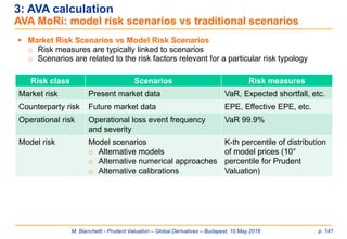
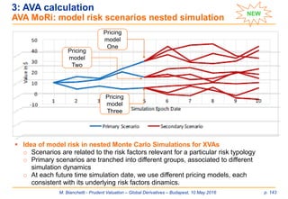
![M. Bianchetti - Prudent Valuation – Global Derivatives – Budapest, 10 May 2016 p. 144
4: AVA calculation
AVA Model Risk (MoRi): case study 1 [1]
Case study 1: model risk in interest rate yield curve construction
Interest rate yield curves are used everywhere for discounting and for interest rate
derivatives and securities with floating rate coupons. So, this is an important case
study.
Yield curve construction is based on recursive application of pricing formulas applied
to interest rate market instruments. So, there is a lot of modelling inside.
In particular, the interpolation algorithm is very important, both pre and post
bootstrapping:
o Simple but non-smooth linear interpolation algorithms are very simple and
robust, but produces irregular forward curves
o Standard spline interpolation is less simple but produces oscillating yield
curves
o Monotonic cubic spline interpolation is regular.](https://image.slidesharecdn.com/prudentvaluation-long-v1-160602205124/85/Prudent-Valuation-144-320.jpg)
![M. Bianchetti - Prudent Valuation – Global Derivatives – Budapest, 10 May 2016 p. 145
4: AVA calculation
AVA Model Risk (MoRi): case study 1 [2]
Linear interpolation on
zero interest rates
Monotonic cubic spline
interpolation on zero
interest rates](https://image.slidesharecdn.com/prudentvaluation-long-v1-160602205124/85/Prudent-Valuation-145-320.jpg)
![M. Bianchetti - Prudent Valuation – Global Derivatives – Budapest, 10 May 2016 p. 146
4: AVA calculation
AVA Model Risk (MoRi): case study 1 [3]
Differences in bps between three different
interpolation algorithms (linear, natural cubic
spline and monotonic cubic spline) for a
portfolio of 3 standard IRS on Euribor 1M, 6M,
12M + 3 standard Basis Swaps.](https://image.slidesharecdn.com/prudentvaluation-long-v1-160602205124/85/Prudent-Valuation-146-320.jpg)
![M. Bianchetti - Prudent Valuation – Global Derivatives – Budapest, 10 May 2016 p. 147
4: AVA calculation
AVA Model Risk (MoRi): case study 2 [1]
Case study 2: model risk experiment with Numerix
Sensitivity of prices to models
o Various dimensions of modelling decisions
o Example of Bermudan swaption pricing with HW1F, HW2F, CIR, and BK models
o Impact of calibration choices
o AVA MoRi for a Bermudan swaption
o Model implied European swaption smile
Impact of changing market environment on model performance
o Handling of negative rates
o Example of floor pricing with very low strikes by using various models
Joint work with Ilja Faerman and Laure Darleguy, Numerix webinar, 12 Nov. 2014,
available at www.numerix.com](https://image.slidesharecdn.com/prudentvaluation-long-v1-160602205124/85/Prudent-Valuation-147-320.jpg)
![M. Bianchetti - Prudent Valuation – Global Derivatives – Budapest, 10 May 2016 p. 148
4: AVA calculation
AVA Model Risk (MoRi): case study 2 [2]
Case study 2: model risk experiment with Numerix (cont’d)
Global modelling approach
Trade
FX spot
Basis
spread
Yield Curve Correlation
Model
underlying
Forward
curve
Swap rate
Risk factor
Short-rate
Distribution
type
NormalLog-normal Mixture
Chi-
squared
Model type HW1F HW2F
Calibration
instruments
Caplets Swaptions
Instruments
configuration
10Y
diagonal
20Y
diagonal
10Y column
10Y diag +
10Y column
CIR BK
CMS
…
…
…
…
…
…](https://image.slidesharecdn.com/prudentvaluation-long-v1-160602205124/85/Prudent-Valuation-148-320.jpg)
![M. Bianchetti - Prudent Valuation – Global Derivatives – Budapest, 10 May 2016 p. 149
4: AVA calculation
AVA Model Risk (MoRi): case study 2 [3]
Case study 2: model risk experiment with Numerix (cont’d)
Experiment
#
Instruments Models Calibrations
Bermudan
swaption
• Coterminal bermudan payer
swaption
• Euribor 6M
• 10Y maturity
• Annual callability
• Sstrike ATM 10Y swap
• OIS discounting
• Hull-White 1 Factor
(HW1F)
• Black-Karasinski (BK)
• Cox-Ingersoll-Ross 1
Factor (CIR1F)
• Hull-White 2 Factors
(HW2F)
• Cox-Ingersoll-Ross 2
Factors (CIR2F)
• Set 1: 10 Y diagonal
swaption ATM
• Set 2: 10Y diagonal
and 1Y column
swaption ATM
• Set 3: 20Y diagonal
and 1Y column
swaption ATM
Caps/Floors
with negative
rates
• 5Y Floor
• Euribor 6M
• Negative and positive strikes
• Yield curves with negative
rates
• Linear interpolation and flat
extrapolation
• SABR interpolation and flat
extrapolation
• Black (analytic)
• Hull-White 1 Factor
(HW1F)
• Shifted Black-Karasinski
(SBK)
• Set 1: Cap volatility
columns for strikes
ATM and 1%
• Set 2: full Cap volatility
surface, with strikes
from 1% to 10%
Joint work with Ilja Faerman and Laure Darleguy, Numerix webinar, 12 Nov. 2014, www.numerix.com](https://image.slidesharecdn.com/prudentvaluation-long-v1-160602205124/85/Prudent-Valuation-149-320.jpg)
![M. Bianchetti - Prudent Valuation – Global Derivatives – Budapest, 10 May 2016 p. 150
4: AVA calculation
AVA Model Risk (MoRi): case study 2 [4]
Overview of results
Prices range from 1.45% to 3.91%
Normal models produce consistently higher PVs for all calibration sets compared to
non-normal models
HW1F
BK
CIR1F
HW2F
CIR2F
0.00%
1.00%
2.00%
3.00%
4.00%
Set1
Set2
Set3
Bermudanswaptionprices
per model and calibrationset](https://image.slidesharecdn.com/prudentvaluation-long-v1-160602205124/85/Prudent-Valuation-150-320.jpg)
![M. Bianchetti - Prudent Valuation – Global Derivatives – Budapest, 10 May 2016 p. 151
4: AVA calculation
AVA Model Risk (MoRi): case study 2 [5]
Results by calibration set
Calibration set 1 (10Y diagonal) produces highest distribution of prices
Average price is fairly stable across different calibration sets
Same model stays consistently below or above the average price for all calibration
sets
1.00%
1.50%
2.00%
2.50%
3.00%
3.50%
4.00%
4.50%
Set1 Set2 Set3
Bermudanswaptionprices per calibrationset
HW1F BK CIR1F HW2F CIR2F Average](https://image.slidesharecdn.com/prudentvaluation-long-v1-160602205124/85/Prudent-Valuation-151-320.jpg)
![M. Bianchetti - Prudent Valuation – Global Derivatives – Budapest, 10 May 2016 p. 152
4: AVA calculation
AVA Model Risk (MoRi): case study 2 [6]
Results by model
HW1F and BK models exhibit lowest variations in prices with changing calibration set
Prices of 1F and 2F models of the same model type can differ significantly
1.00%
1.50%
2.00%
2.50%
3.00%
3.50%
4.00%
4.50%
HW1F BK CIR1F HW2F CIR2F
Bermudanswaptionprices per model
Set1 Set2 Set3](https://image.slidesharecdn.com/prudentvaluation-long-v1-160602205124/85/Prudent-Valuation-152-320.jpg)
![M. Bianchetti - Prudent Valuation – Global Derivatives – Budapest, 10 May 2016 p. 153
4: AVA calculation
AVA Model Risk (MoRi): case study 2 [7]
Results
Notional is 10m EUR
Assuming Fair Value is the average of all price
Long swaption:
o Fair Value: FV = 258k EUR
o Prudent value is the 10% percentile of all prices: PV = 177k EUR
o AVA MoRi = 0.5x(FV-PV) = 40.5k EUR
Short swaption:
o Fair Value: FV = -258k EUR
o Prudent value is the 90% percentile of all prices: PV = -317k EUR
o AVA MoRi = 0.5x(FV-PV) = 29.5k EUR](https://image.slidesharecdn.com/prudentvaluation-long-v1-160602205124/85/Prudent-Valuation-153-320.jpg)
![M. Bianchetti - Prudent Valuation – Global Derivatives – Budapest, 10 May 2016 p. 154
4: AVA calculation
AVA Model Risk (MoRi): case study 2 [8]
Excluding models
All models All except HW2F All models All except HW2F
Fair Value (1) 258 258 -258 -258
Prudent Value 177 158 -317 -315
Model Risk AVA 40.5 50 29.5 28.5
Long swaption Short swaption
Fair Value (1) is computed as the average of all model prices
Fair Value (2) for “All except HW2F” is computed excluding the price of the HW2F model
All models All except HW2F All models All except HW2F
Fair Value (2) 258 240 -258 -240
Prudent Value 177 158 -317 -315
Model Risk AVA 40.5 41 29.5 37.5
Short swaptionLong swaption](https://image.slidesharecdn.com/prudentvaluation-long-v1-160602205124/85/Prudent-Valuation-154-320.jpg)
![M. Bianchetti - Prudent Valuation – Global Derivatives – Budapest, 10 May 2016 p. 155
4: AVA calculation
AVA Model Risk (MoRi): case study 2 [9]
Exercise probabilities
0.00%
10.00%
20.00%
30.00%
40.00%
50.00%
60.00%
70.00%
80.00%
Oct-15 Oct-16 Oct-17 Oct-18 Oct-19 Oct-20 Oct-21 Oct-22 Oct-23
Call probabilities per coupon
Calibrationset1
HW1F
BK
CIR
HW2F
CIR2F
0.00%
10.00%
20.00%
30.00%
40.00%
50.00%
60.00%
70.00%
80.00%
Oct-15 Oct-16 Oct-17 Oct-18 Oct-19 Oct-20 Oct-21 Oct-22 Oct-23
Call probabilities per coupon
Calibrationset2
HW1F
BK
CIR
HW2F
CIR2F
0.00%
10.00%
20.00%
30.00%
40.00%
50.00%
60.00%
70.00%
80.00%
Oct-15 Oct-16 Oct-17 Oct-18 Oct-19 Oct-20 Oct-21 Oct-22 Oct-23
Call probabilities per coupon
Calibrationset3
HW1F
BK
CIR
HW2F
CIR2F
Exercise probability per coupon
CIR-type models imply a higher
probability of early exercise than HW
models
The term structure of exercise
probabilities is regular for all models for
calibration set 1, humped for calibration
sets 2 and 3.](https://image.slidesharecdn.com/prudentvaluation-long-v1-160602205124/85/Prudent-Valuation-155-320.jpg)
![M. Bianchetti - Prudent Valuation – Global Derivatives – Budapest, 10 May 2016 p. 156
AVA definition
AVA Unearned Credit Spread (UCS) refers to the valuation uncertainty in the credit
valuation adjustment (CVA) to include, according to the applicable accounting
framework, the current value of expected losses due to counterparty default on
derivative positions. Such valuation uncertainty refers, in particular, to MPU, CoCo
and MoRi uncertainties in the calculation of CVA. Hence, the RTS specifies that the
AVA UCS shall be split into such components, to be aggregated to their
corresponding AVA.
Since the definition of AVA UCS specifies “losses due to counterparty default” (not
“profits due to own default”), and the CRR, art. 33 states that the debt valuation
adjustment (DVA, the gain on liabilities due to own credit quality) should not be
included in the calculation of own funds, then AVA UCS shall not include the DVA
component.
AVA main references
o EBA RTS, article 12.
o EBA FAQs 10, 25, 28.
4: AVA calculation
AVA Unearned Credit Spread (UCS) [1]](https://image.slidesharecdn.com/prudentvaluation-long-v1-160602205124/85/Prudent-Valuation-156-320.jpg)
![M. Bianchetti - Prudent Valuation – Global Derivatives – Budapest, 10 May 2016 p. 157
AVA scope of application
Within the general prudent valuation scope (see before), AVA UCS refers in particular
to those valuation positions subject to a credit valuation adjustment, and specifically,
to OTC derivatives, with a particular focus on uncollateralized derivatives. Securities
are excluded, since credit risk is already included in the security credit spread.
AVA Fair Value
The FV of the trades subject to AVA UCS may include full, partial or null CVA. In any
case the FV subject to prudent valuation for AVA UCS must include these CVAs.
4: AVA calculation
AVA Unearned Credit Spread (UCS) [2]](https://image.slidesharecdn.com/prudentvaluation-long-v1-160602205124/85/Prudent-Valuation-157-320.jpg)
![M. Bianchetti - Prudent Valuation – Global Derivatives – Budapest, 10 May 2016 p. 158
4: AVA calculation
AVA Unearned Credit Spread (UCS) [3]
AVA Unearned Credit Spread (UCS) (EBA RTS, article 12) refers to the valuation uncertainty in
the credit valuation adjustment to include, according to the applicable accounting framework, the
current value of expected losses due to counterparty default on derivative positions.
o Is the valuation position 𝑝𝑖, 𝑖 = 1, … , 𝑁𝑝, a derivative position, and
o according to the applicable accounting framework, is an
adjustment necessary to include the current value of expected
losses due to counterparty default (CVA) ?
YES
NO
𝐴𝑃𝑉𝐴 𝑈𝐶𝑆 𝑡, 𝑝𝑖 = 0
Aggregate
𝐴𝑃𝑉𝐴 𝑈𝐶𝑆 𝑡, 𝑝𝑖, 𝑀𝑃𝑈
to APVA MPU.
Go to AVA MPU and apply
those rules to compute
individual AVA UCS w.r.t.
MPU, 𝐴𝑃𝑉𝐴 𝑈𝐶𝑆 𝑡, 𝑝𝑖, 𝑀𝑃𝑈
Aggregate
𝐴𝑃𝑉𝐴 𝑈𝐶𝑆 𝑡, 𝑝𝑖, 𝐶𝑜𝐶𝑜
to APVA CoCo.
Go to AVA CoCo and apply
those rules to compute
individual AVA UCS w.r.t.
CoCo, 𝐴𝑃𝑉𝐴 𝑈𝐶𝑆 𝑡, 𝑝𝑖, 𝐶𝑜𝐶𝑜
Aggregate
𝐴𝑃𝑉𝐴 𝑈𝐶𝑆 𝑡, 𝑝𝑖, 𝑀𝑜𝑅𝑖
to APVA MoRi.
Go to AVA MoRi and apply
those rules to compute
individual AVA UCS w.r.t.
MoRi, 𝐴𝑃𝑉𝐴 𝑈𝐶𝑆 𝑡, 𝑝𝑖, 𝑀𝑜𝑅𝑖](https://image.slidesharecdn.com/prudentvaluation-long-v1-160602205124/85/Prudent-Valuation-158-320.jpg)
![M. Bianchetti - Prudent Valuation – Global Derivatives – Budapest, 10 May 2016 p. 159
AVA calculation
o Securities: excluded
o Derivatives
• DVA component
𝐴𝑉𝐴 𝑈𝐶𝑆 𝑡 = 0, since DVA is excluded from the prudent valuation scope.
• CVA component
𝐴𝑉𝐴 𝑈𝐶𝑆 𝑡 shall be calculated considering the following components.
Unilateral CVA: since DVA is excluded, Institutions shall consider the
unilateral CVA, without first to default conditioning.
𝐴𝑉𝐴 𝑈𝐶𝑆 𝑡, 𝑀𝑃𝑈 : uncertainty in CDS spreads, PDs and recovery rates,
uncertainty in risk factors used to compute the exposure (e.g. curves,
volatilities)
𝐴𝑉𝐴 𝑈𝐶𝑆 𝑡, 𝐶𝑜𝐶𝑜 : bid/ask in CDS spreads.
𝐴𝑉𝐴 𝑈𝐶𝑆 𝑡, 𝑀𝑜𝑅𝑖 : unilateral vs bilateral CVA, time simulation grid, risk free vs
risky close-out, wrong way risk, different dynamics to simulate underlying risk
factors and compute the exposure.
• No CVA case
if the CVA is not included in the accounting fair value for some valuation
positions, 𝐴𝑉𝐴 𝐶𝑉𝐴 𝑡 shall be equal to the full CVA of those position, calculated
using prudent parameters as above.
4: AVA calculation
AVA Unearned Credit Spread (UCS) [4]](https://image.slidesharecdn.com/prudentvaluation-long-v1-160602205124/85/Prudent-Valuation-159-320.jpg)
![M. Bianchetti - Prudent Valuation – Global Derivatives – Budapest, 10 May 2016 p. 160
AVA definition
AVA Investing and Funding Costs (IFC) refers to the valuation uncertainty in the
funding costs used when assessing the exit price of a valuation position, according to
the applicable accounting framework.
Such valuation uncertainty refers, in particular, to MPU, CoCo and MoRi
uncertainties in the calculation of the funding cost. Hence, AVA IFC shall be split into
such components, to be aggregated to their corresponding AVAs.
AVA main references
o EBA RTS, article 13.
o EBA FAQs 26, 35, 36.
AVA scope of application
Within the general prudent valuation scope (see before), AVA IFC refers in particular
to those valuation positions subject to a funding valuation adjustment and
specifically, to OTC derivatives. Securities are excluded, since funding risk is already
included in the security credit spread
AVA Fair Value
The FV of the trades subject to AVA IFC may include full, partial or null FVA. In any
case the FV subject to prudent valuation for AVA IFC must include these FVAs.
4: AVA calculation
AVA Investing and Funding Costs (IFC) [1]](https://image.slidesharecdn.com/prudentvaluation-long-v1-160602205124/85/Prudent-Valuation-160-320.jpg)
![M. Bianchetti - Prudent Valuation – Global Derivatives – Budapest, 10 May 2016 p. 161
4: AVA calculation
AVA Investing and Funding Costs (IFC) [2]
AVA Investing and Funding Cost (IFC) (EBA RTS, article 13)
refers to the valuation uncertainty in the funding costs used when assessing the exit price
according to the applicable accounting framework
o Is the valuation position 𝑝𝑖, 𝑖 = 1, … , 𝑁𝑝, a derivative position, and
o according to the applicable accounting framework, is an
adjustment necessary to include the funding costs in the exit
price (FVA) ?
YES
NO 𝐴𝑃𝑉𝐴𝐼𝐹𝐶 𝑡, 𝑝𝑖 = 0
Aggregate
𝐴𝑃𝑉𝐴𝐼𝐹𝐶 𝑡, 𝑝𝑖, 𝑀𝑃𝑈
to APVA MPU.
Go to AVA MPU and apply
those rules to compute
individual AVA IFC w.r.t.
MPU, 𝐴𝑃𝑉𝐴𝐼𝐹𝐶 𝑡, 𝑝𝑖, 𝑀𝑃𝑈
Aggregate
𝐴𝑃𝑉𝐴𝐼𝐹𝐶 𝑡, 𝑝𝑖, 𝐶𝑜𝐶𝑜
to APVA CoCo.
Go to AVA CoCo and apply
those rules to compute
individual AVA IFC w.r.t.
CoCo, 𝐴𝑃𝑉𝐴𝐼𝐹𝐶 𝑡, 𝑝𝑖, 𝐶𝑜𝐶𝑜
Aggregate
𝐴𝑃𝑉𝐴𝐼𝐹𝐶 𝑡, 𝑝𝑖, 𝑀𝑜𝑅𝑖
to APVA MoRi.
Go to AVA MoRi and apply
those rules to compute
individual AVA IFC w.r.t.
MoRi, 𝐴𝑃𝑉𝐴𝐼𝐹𝐶 𝑡, 𝑝𝑖, 𝑀𝑜𝑅𝑖](https://image.slidesharecdn.com/prudentvaluation-long-v1-160602205124/85/Prudent-Valuation-161-320.jpg)
![M. Bianchetti - Prudent Valuation – Global Derivatives – Budapest, 10 May 2016 p. 162
AVA calculation
o Securities: excluded
o Derivatives
• Strongly collateralized derivatives
𝐴𝑉𝐴 𝐹𝑉𝐴 𝑡 = 0 if the funding cost is already included in the FV using OIS
discounting methodology.
• Non-Strongly collateralized derivatives
If the FVA is included in the accounting FV for some valuation positions, AVA
IFC shall be calculated as the FVA uncertainty, resulting from the uncertainty
in the funding curve.
If the FVA is not included in the accounting FV for some valuation positions,
𝐴𝑉𝐴 𝐹𝑉𝐴 𝑡 shall be equal to the full FVA of those position, calculated using
prudent parameters.
• CSA with initial margins
AVA IFC shall computed on the initial margins, using a discounting approach
applied to an exposure profile assigned to the future initial margin.
4: AVA calculation
AVA Investing and Funding Costs (IFC) [3]](https://image.slidesharecdn.com/prudentvaluation-long-v1-160602205124/85/Prudent-Valuation-162-320.jpg)
![M. Bianchetti - Prudent Valuation – Global Derivatives – Budapest, 10 May 2016 p. 163
4: AVA calculation
AVA Investing and Funding Costs (IFC) [4]
• 𝐴𝑉𝐴𝐼𝐹𝐶 𝑡 shall be calculated considering the following components.
𝐴𝑉𝐴𝐼𝐹𝐶 𝑡, 𝑀𝑃𝑈 : uncertainty in funding spreads, PDs and recovery rates,
uncertainty in risk factors used to compute the exposure (e.g. curves,
volatilities)
𝐴𝑉𝐴𝐼𝐹𝐶 𝑡, 𝐶𝑜𝐶𝑜 : bid/ask in funding spreads.
𝐴𝑉𝐴𝐼𝐹𝐶 𝑡, 𝑀𝑜𝑅𝑖 : time simulation grid, different dynamics to simulate
underlying risk factors and compute the exposure.
Funding spread estimation
AVA IFC calculation is based on the estimation of a prudent funding curve. Possible
sources of such yield curve is the bond yield curve based on own Institution bond
emissions.](https://image.slidesharecdn.com/prudentvaluation-long-v1-160602205124/85/Prudent-Valuation-163-320.jpg)
![M. Bianchetti - Prudent Valuation – Global Derivatives – Budapest, 10 May 2016 p. 164
4: AVA calculation
AVA Investing and Funding Costs (IFC) [5]
Switch to FVA accounting
“[JPM] implemented a FVA framework this quarter for its OTC derivatives and structured notes,
reflecting an industry migration towards incorporating the cost or benefit of unsecured funding
into valuations. For the first time this quarter, we were able to clearly observe the existence of
funding costs in market clearing levels. As a result, the firm recorded a $1.5 billion loss this
quarter.” (source: M. Cameron, Risk Magazine, 14 Jan. 2014)
Bank 2012 2013
Barclays -£101 MM ?
Deutsche Bank -- -€364 MM
Goldman Sachs ? ?
JP Morgan -- -$1.500 MM
Lloyds Banking Group - £143 MM -£135 MM
Nomura -- -¥10.000 MM (-$98 MM)
Royal Bank of Scotland - £475 MM -£424 MM
Societè Generale ? ?
UBS -- --](https://image.slidesharecdn.com/prudentvaluation-long-v1-160602205124/85/Prudent-Valuation-164-320.jpg)
![M. Bianchetti - Prudent Valuation – Global Derivatives – Budapest, 10 May 2016 p. 165
AVA definition
AVA Concentrated Positions (CoPo) refers to the valuation uncertainty in the exit
price of concentrated positions.
Such valuation uncertainty refers, in particular, to those valuation positions showing
concentrated exposures related to:
o the size relative to the liquidity of the related market;
o the average daily market volume and typical daily trading volume of the institution;
o the institution’s ability to trade in that market, and to exit the valuation position
within the time horizon implied by the market risk capitalization (10 days) without
impacting the market.
AVA main references
o EBA RTS, article 14.
o EBA FAQs 32, 33, 34.
AVA scope of application
Within the general prudent valuation scope (see before), AVA CoPo refers in
particular to those valuation positions subject to concentration risk as defined above.
AVA Fair Value
The FV of the trades subject to AVA CoPo typically does not include a CoPo
component.
3: AVA calculation
AVA Concentrated Positions (CoPo) [1]](https://image.slidesharecdn.com/prudentvaluation-long-v1-160602205124/85/Prudent-Valuation-165-320.jpg)
![M. Bianchetti - Prudent Valuation – Global Derivatives – Budapest, 10 May 2016 p. 166
3: AVA calculation
AVA Concentrated Positions (CoPo) [2]
AVA Concentrated Positions (CoPo) (EBA RTS, article 14)
refers to the valuation uncertainty in the exit price of concentrated positions
Identify concentrated valuation positions 𝑝𝑖, 𝑖 = 1, … , 𝑁𝑝, considering:
o the size of all valuation positions relative to the liquidity of their related market,
o the institution’s ability to trade in that market,
o the average daily market volume and typical daily trading volume of the institution.
YES
NO
𝐴𝑃𝑉𝐴 𝐶𝑜𝑃𝑜 𝑡, 𝑝𝑖 = 0
For each concentrated valuation position 𝑝𝑖, there exists
a market price applicable for the size of the position ?
Estimate a prudent exit period
Does the prudent exit period exceed 10 days ?
Continue
YES
NO](https://image.slidesharecdn.com/prudentvaluation-long-v1-160602205124/85/Prudent-Valuation-166-320.jpg)
![M. Bianchetti - Prudent Valuation – Global Derivatives – Budapest, 10 May 2016 p. 167
3: AVA calculation
AVA Concentrated Positions (CoPo) [3]
Compute individual AVA CoPo taking into
account:
o the volatility of the valuation input,
o the volatility of the bid offer spread,
o the impact of the hypothetical exit
strategy on market prices.
Document the methodology
applied to determine
concentrated valuation positions
for which a concentrated
positions AVA is calculated
Compute total category level AVA CoPo
𝐴𝑉𝐴 𝐶𝑜𝑃𝑜 𝑡 =
𝑖=1
𝑁 𝑝
𝐴𝑃𝑉𝐴 𝐶𝑜𝑃𝑜 𝑡, 𝑝𝑖](https://image.slidesharecdn.com/prudentvaluation-long-v1-160602205124/85/Prudent-Valuation-167-320.jpg)
![M. Bianchetti - Prudent Valuation – Global Derivatives – Budapest, 10 May 2016 p. 168
AVA calculation
o Securities
AVA CoPo may be calculated as follows:
• Look for possible concentrated positions by comparing the size held w.r.t. the
outstanding amount of the security circulating on the market,
• estimate coefficients of uncertainty related to the sizes above,
• compute AVA CoPo via sensitivity on the credit risk factors and uncertainties
above.
o Derivatives
OTC derivatives typically do not show concentrated positions in the sense defined
above. Possible exceptions shall be documented and AVA CoPo shall be
calculated as described in the previous scheme.
Examples
o Concentrated positions into single stock w.r.t. typical stock trading volumes
o Concentrated positions into single bond emissions w.r.t. typical bond trading
volumes and outstanding amount.
3: AVA calculation
AVA Concentrated Positions (CoPo) [4]
w.r.t. typical stock trading volumes](https://image.slidesharecdn.com/prudentvaluation-long-v1-160602205124/85/Prudent-Valuation-168-320.jpg)
![M. Bianchetti - Prudent Valuation – Global Derivatives – Budapest, 10 May 2016 p. 169
AVA definition
AVA FAC takes into account the valuation uncertainty emerging from possible
administrative costs and future hedging costs on valuation positions for which a
direct exit price is not applied for the close-out costs AVA. Thus, future administrative
costs are complementary to close-out costs. If the close-out costs are assessed on a
full exit price basis then, after executing the corresponding close out strategy, the
positions disappear, and there are no future administrative costs. However, where
close-out costs are assessed on a "cost-to hedge" basis, as with derivative portfolios,
the positions are maintained, and therefore there are possible future administrative
costs in running the portfolio until maturity.
AVA main references
o EBA RTS, article 15.
o EBA FAQs 37, 37.1.
AVA scope of application
Within the general prudent valuation scope (see before), AVA CoPo refers in
particular to those valuation positions subject to FAC as defined above.
4: AVA calculation
AVA Future Administrative Costs (FAC) [1]](https://image.slidesharecdn.com/prudentvaluation-long-v1-160602205124/85/Prudent-Valuation-169-320.jpg)
![M. Bianchetti - Prudent Valuation – Global Derivatives – Budapest, 10 May 2016 p. 170
AVA Fair Value
The FV of the valuation positions typically does not include the effect of possible
future administrative costs, since such costs are specific of each institution and do
not regard an exit price according to IFRS. Hence, the AVA FAC must be applied
directly to the full FV of valuation positions.
4: AVA calculation
AVA Future Administrative Costs (FAC) [2]](https://image.slidesharecdn.com/prudentvaluation-long-v1-160602205124/85/Prudent-Valuation-170-320.jpg)
![M. Bianchetti - Prudent Valuation – Global Derivatives – Budapest, 10 May 2016 p. 171
4: AVA calculation
AVA Future Administrative Costs (FAC) [3]
AVA Future Administrative Costs (FAC) (EBA RTS, article 15)
refers to the valuation uncertainty due to future administrative and hedging costs
YES 𝐴𝑃𝑉𝐴 𝐹𝐴𝐶 𝑡, 𝑝𝑖 = 0
Do you calculate 𝐴𝑃𝑉𝐴 𝑀𝑃𝑈 and 𝐴𝑃𝑉𝐴 𝐶𝑜𝐶𝑜 for a valuation
exposure 𝑝𝑖, 𝑖 = 1, … , 𝑁𝑝,, which imply fully exiting the exposure ?
Compute individual APVA FAC taking into account:
o administrative costs, including all incremental staffing and fixed costs that will be incurred in
managing the portfolio, over the expected life of the valuation exposures,
o the future hedging costs over the expected life of the valuation exposures,
o the cost reduction as long as the size of the valuation exposure reduces,
o the term structure of discounts at risk free rate.
NO
Compute total category level AVA FAC
𝐴𝑉𝐴 𝐹𝐴𝐶 𝑡 =
𝑖=1
𝑁 𝑝
𝐴𝑃𝑉𝐴 𝐹𝐴𝐶 𝑡, 𝑝𝑖](https://image.slidesharecdn.com/prudentvaluation-long-v1-160602205124/85/Prudent-Valuation-171-320.jpg)
![M. Bianchetti - Prudent Valuation – Global Derivatives – Budapest, 10 May 2016 p. 172
4: AVA calculation
AVA Future Administrative Costs (FAC) [4]
AVA calculation
Considering the regulatory requirements, we may write a general formula for AVA
FAC
𝐴𝑃𝑉𝐴 𝐹𝐴𝐶 𝑡, 𝑝𝑖 = න
𝑡
𝑇
𝑃 𝑡, 𝑢 𝐴𝑑𝐶 𝑡, 𝑢, 𝑝𝑖 𝑁 𝐹𝐴𝐶 𝑡, 𝑢, 𝑝𝑖 𝑑𝑢
where
o 𝑃 𝑡, 𝑢 = discount factor over the time interval 𝑡, 𝑢 ,
o 𝐴𝑑𝐶 𝑡, 𝑢, 𝑝𝑖 = administrative costs expected at time t for future time interval
𝑢, 𝑢 + 𝑑𝑢 , per unit of currency,
o 𝑁 𝐹𝐴𝐶 𝑡, 𝑢, , 𝑝𝑖 = nominal of the valuation exposure at future time u,
o T = exipry date of the valuation exposure
Considering constant administrative costs and a decreasing step-wise constant
notional struck on dates 𝑇1, … , 𝑇 𝑀 , 𝑡 < 𝑇1, 𝑇 𝑀 = 𝑇, we may write a discrete formula
𝐴𝑃𝑉𝐴 𝐹𝐴𝐶 𝑡, 𝑝𝑖 ≅ 𝐴𝑑𝐶 𝑡, 𝑝𝑖
𝑘=𝑇1
𝑇 𝑀
𝑃 𝑡, 𝑇𝑘 𝑁 𝐹𝐴𝐶 𝑡, 𝑇𝑘, 𝑝𝑖 𝑇𝑘 − 𝑇𝑘−1 .
Considering furthermore a single (weighted) average lifetime 𝑇𝑎𝑣𝑔 (WAL) we may
further simplify to
𝐴𝑃𝑉𝐴 𝐹𝐴𝐶 𝑡, 𝑝𝑖 ≅ 𝐴𝑑𝐶 𝑡 𝑃 𝑡, 𝑇𝑎𝑣𝑔 𝑁 𝐹𝐴𝐶 𝑡, 𝑇𝑎𝑣𝑔 𝑇𝑎𝑣𝑔 − 𝑡 .](https://image.slidesharecdn.com/prudentvaluation-long-v1-160602205124/85/Prudent-Valuation-172-320.jpg)
![M. Bianchetti - Prudent Valuation – Global Derivatives – Budapest, 10 May 2016 p. 173
4: AVA calculation
AVA Future Administrative Costs (FAC) [5]
AVA calculation (cont’d)
Clearly, the administrative cost 𝐴𝑑𝐶 𝑡, 𝑝𝑖 is the most difficult data to obtain. We
stress that in the formula above 𝐴𝑑𝐶 𝑡, 𝑝𝑖 refers to the cost per unit of time and
currency, not to the total cost of the desk or the institution, which manage other
portfolios not subject to AVA.
AVA data
AVA FAC calculations require the following input data.
o Valuation positions not at full exit price, with nominal amounts and maturities.
o Administrative and hedging costs per unit of time, per currency, per desk, per
activity.
o Risk free (OIS) discount term structure until portfolio maturity.](https://image.slidesharecdn.com/prudentvaluation-long-v1-160602205124/85/Prudent-Valuation-173-320.jpg)
![M. Bianchetti - Prudent Valuation – Global Derivatives – Budapest, 10 May 2016 p. 174
AVA definition
AVA Early Termination (EaT) refers to the valuation uncertainty emerging from
potential losses arising from non-contractual early terminations of client trades.
AVA main references
o EBA RTS, article 16.
o EBA FAQs 38.
AVA scope of application
Within the general prudent valuation scope (see before), AVA EaT regards in
particular client trades, that is, trades with client counterparties that may be subject
to non-contractual early termination because of litigations or commercial reasons.
AVA Fair Value
The FV of the client trades subject to AVA EaT typically does not include the effect of
possible non-contractual early terminations by clients. In some particular cases,
Institutions may account reserves in their balance sheets to cover possible losses
related to early terminations of some trades or portfolios with specific counterparties.
If these reserves are accounted as a FV component, the FV subject to prudent
valuation for AVA EaT must include the reserves. In other words, the reserves must
be subtracted from the AVA EaT.
4: AVA calculation
AVA Early Termination (EaT) [1]](https://image.slidesharecdn.com/prudentvaluation-long-v1-160602205124/85/Prudent-Valuation-174-320.jpg)
![M. Bianchetti - Prudent Valuation – Global Derivatives – Budapest, 10 May 2016 p. 175
4: AVA calculation
AVA Early Termination (EaT) [2]
AVA Early Termination (ET) (EBA RTS, article 16)
reflects the valuation uncertainty arising from potential losses
due to possible non-contractual early terminations of client trades.
YES
Is the valuation position 𝑝𝑖, 𝑖 = 1, … , 𝑁𝑝,
subject to possible non-contractual early termination ?
Identify a suitable past time window 𝑇; 𝑡 and historical trades 𝑢𝑗 =
1, … , 𝑁𝐸𝑎𝑇 subject to non-contractual early terminations at past dates
𝑇 𝑁 𝐸𝑎𝑇
, … , 𝑇1 such that 𝑇 ≤ 𝑇 𝑁 𝐸𝑎𝑇
≤ ⋯ ≤ 𝑇1 ≤ 𝑡.
NO
Retrieve the corresponding historical fair values 𝐹𝑉 𝑇𝑗, 𝑢𝑗
and actual termination prices 𝑃 𝑇𝑗, 𝑢𝑗 .
Continue
𝐴𝑃𝑉𝐴 𝐸𝑎𝑇 𝑡, 𝑝𝑖 = 0](https://image.slidesharecdn.com/prudentvaluation-long-v1-160602205124/85/Prudent-Valuation-175-320.jpg)
![M. Bianchetti - Prudent Valuation – Global Derivatives – Budapest, 10 May 2016 p. 176
4: AVA calculation
AVA Early Termination (EaT) [3]
The 10th percentile
may be negative (loss)
or positive (profit), and
represents the highest
loss or the smallest
profit realized with
90% historical
probability.
Compute individual APVA EaT according to the formula
𝐴𝑃𝑉𝐴 𝐸𝑎𝑇 𝑡, 𝑝𝑖 = ቊ
0, 𝑖𝑓 𝑃𝐿10% ≥ 0,
𝑃𝐿10% × 𝐹𝑉 𝑡, 𝑝𝑖 𝑖𝑓 𝑃𝐿10% < 0.
Calculate
o the historical profit and loss values, 𝑃𝐿 𝑇𝑗, 𝑢𝑗 ∶= ൗ𝑃 𝑇𝑗, 𝑢𝑗 − 𝐹𝑉 𝑇𝑗, 𝑢𝑗 𝐹𝑉 𝑇𝑗, 𝑢𝑗 ,
o the historical P&L distribution, ΤΔ𝑁 Δ𝑃𝐿 ,
o the 10th percentile of the P&L distribution, 𝑃𝐿10% ≔ ℙ ΤΔ𝑁 Δ𝑃𝐿 , 10% ,
Compute total category level AVA EaT
𝐴𝑉𝐴 𝐸𝑎𝑇 𝑡 =
𝑖=1
𝑁 𝑝
𝐴𝑃𝑉𝐴 𝐸𝑎𝑇 𝑡, 𝑝𝑖](https://image.slidesharecdn.com/prudentvaluation-long-v1-160602205124/85/Prudent-Valuation-176-320.jpg)
![M. Bianchetti - Prudent Valuation – Global Derivatives – Budapest, 10 May 2016 p. 177
4: AVA calculation
AVA Early Termination (EaT) [4]
AVA calculation
See flow chart above.
AVA data
AVA EaT calculations require a database of historical early terminations, including,
for each trade:
o termination date,
o nominal,
o fair value at EaT time instant,
o actual EaT price at EaT time instant.
Examples
o Trades early terminated because of litigations
o Trades early terminated because of commercial relationships](https://image.slidesharecdn.com/prudentvaluation-long-v1-160602205124/85/Prudent-Valuation-177-320.jpg)
![M. Bianchetti - Prudent Valuation – Global Derivatives – Budapest, 10 May 2016 p. 178
4: AVA calculation
AVA Early Termination (EaT) [5]
Case study
See figure below.](https://image.slidesharecdn.com/prudentvaluation-long-v1-160602205124/85/Prudent-Valuation-178-320.jpg)
![M. Bianchetti - Prudent Valuation – Global Derivatives – Budapest, 10 May 2016 p. 179
4: AVA calculation
AVA Early Termination (EaT) [6]
Case study (cont’d)
o The nominal of the present portfolio of client trades subject to possible non-contractual EaT
(cols. 2-4 top, 12 €mln) is taken from “Derivatives HFT” in the sample portfolio.
o The absolute FV is set to 5% of the nominal for 1,000 trades.
o The past portfolio is set to half the present portfolio and may be seen as an average over the
EaT historical window (so, trading volume increased from past to present).
o The portfolio of client trades that were historically early terminated (cols. 5-7 top) is set to 1%
of the past portfolio, hence the historical probability of non-contractual EaT is 1%.
o In the bottom table we show a possible drill-down of the 10 trades historically affected by
non-contractual EaT. We generated the absolute EaT price (col. 4) as P=FV(1+10%ε), where
ε is a random number with uniform distribution in [-1,1].
o Hence, the P&L (cols. 5-6) may be positive or negative (we chose a negative case).
o Given the relative P&L% distribution (col. 6), we calculated the 10th percentile (which, in this
simple case with 10 trades, is just the 2nd higher P&L%), representing the highest loss
happened with 90% historical probability after non-contractual EaT.
o Finally, we applied such historical estimate to the absolute FV of the present portfolio in the
top table (col. 9-10).
o The AVA (col. 11) is just the absolute value of the corresponding expected loss (col. 9).
o We notice that the historical P&L%(10) (-9.64%) corresponds to a small historical loss (-
28,917€) originated by a single deal with limited fair value (300.000€) but generates a much
larger expected loss (-578,346€) once applied to the fair value of the present portfolio
(6,000,000€). This is consistent with the idea of prudent value at 90% confidence level
required by the regulation.](https://image.slidesharecdn.com/prudentvaluation-long-v1-160602205124/85/Prudent-Valuation-179-320.jpg)
![M. Bianchetti - Prudent Valuation – Global Derivatives – Budapest, 10 May 2016 p. 180
AVA definition
AVA Early Termination (EaT) takes into account the valuation uncertainty emerging
from potential losses that an institution may incur because of the operational risk
related to valuation processes. This risk is mainly related, but not limited, to the
balance sheet substantiation process and to possible legal disputes (RTS art. 17.1).
The main driver for AVA OpR is the operational risk framework adopted by the
Institution. Institutions adopting the Advanced Measurement Approach (AMA)
Operational Risk defined in the CRR, title III, ch. 4, art. 321-324 (AMA Institutions)
are allowed a lighter AVA OpR, as described below. This facilitation is intended to
avoid double counting of capital reserves related to the same source of risk. In all
other cases (non-AMA Institutions), the AVA OpR is given by 10% of the sum of AVA
MPU and AVA CoCo, which can result in high figures. In particular, FAQ 39, remarks
that Institutions using the Standardized Method for Operational Risk defined in the
CRR, title III, ch. 3, art. 317-320, cannot show that they already take into account the
operational risk related to valuation processes. Thus they are not allowed to
calculate AVA OpR as AMA institutions. .
AVA main references
o EBA RTS, article 17.
o EBA FAQs 39, 40, 42.
4: AVA calculation
AVA Operational Risk (OpR) [1]](https://image.slidesharecdn.com/prudentvaluation-long-v1-160602205124/85/Prudent-Valuation-180-320.jpg)
![M. Bianchetti - Prudent Valuation – Global Derivatives – Budapest, 10 May 2016 p. 181
AVA scope of application
Within the general prudent valuation scope (see before), AVA OpR regards in
particular those positions that:
o can be considered subject to operational risk during the valuation process;
o for which in the balance sheet there are provisions for operational risk.
Evidences of operational risk related to valuation process are the inclusion of those
valuation processes as part of the AMA accounting for the mispricing, misselling and
the process execution errors. Furthermore, an AMA usually accounts provision for
legal disputes with clients where the underlying of the contract is a fair value position.
AVA Fair Value
The fair values of positions under AVA OpR typically does not include any component
or adjustment related to operational risk, since these factors do not concur to an exit
price. From a risk management point of view, expected operational risk losses may
be evaluated using scenario analysis and historical data related to realized
operational risk losses.
4: AVA calculation
AVA Operational Risk (OpR) [2]](https://image.slidesharecdn.com/prudentvaluation-long-v1-160602205124/85/Prudent-Valuation-181-320.jpg)
![M. Bianchetti - Prudent Valuation – Global Derivatives – Budapest, 10 May 2016 p. 182
4: AVA calculation
AVA Operational Risk (OpR) [3]
AVA Early Termination (ET) (EBA RTS, article 17) reflects the
reflects the valuation uncertainty arising from potential losses
that may be incurred as a result of operational risk related to valuation processes.
Identify valuation positions 𝑝𝑖, 𝑖 = 1, … , 𝑁𝑝, judged to be at-risk during the balance sheet
substantiation process, including those due to legal disputes.
Compute individual APVA OpR according to the formula
𝐴𝑃𝑉𝐴 𝑂𝑝𝑅 𝑡, 𝑝𝑖 = 10% × 𝐴𝑃𝑉𝐴 𝑀𝑃𝑈 𝑡, 𝑝𝑖 + 𝐴𝑃𝑉𝐴 𝐶𝑜𝐶𝑜 𝑡, 𝑝𝑖
Is the AMA (Advanced Measurement Approach) applied to Operational Risk (as defined
in Title III Chapter 4 of Regulation (EU) No 575/2013) for valuation positions 𝑝𝑖 ?
Is there evidence that the operational risk relating to valuation processes of valuation
positions 𝑝𝑖 is fully accounted for by the AMA calculation ?
YES
NO
𝐴𝑃𝑉𝐴 𝑂𝑝𝑅 𝑡, 𝑝𝑖 = 0
NO
YES
Compute total category level AVA OpR
𝐴𝑉𝐴 𝑂𝑝𝑅 𝑡 =
𝑖=1
𝑁 𝑝
𝐴𝑃𝑉𝐴 𝑂𝑝𝑅 𝑡, 𝑝𝑖](https://image.slidesharecdn.com/prudentvaluation-long-v1-160602205124/85/Prudent-Valuation-182-320.jpg)
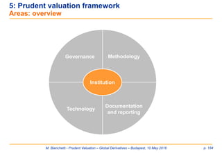
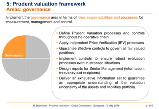
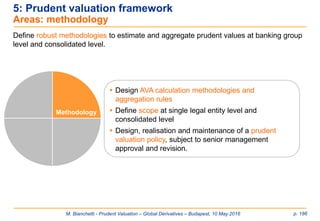
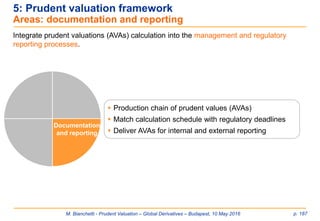
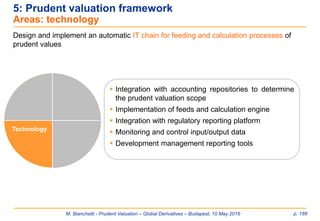
![M. Bianchetti - Prudent Valuation – Global Derivatives – Budapest, 10 May 2016 p. 189
5: Prudent valuation framework
Example of Prudent Valuation framework [1/4]
Scope Calculation Reporting
Identify fair value positions
Apply exlusionsprovided by the regulator:
o Positions subject to prudential filters such that fiar
value variations has no or partial impact on CET1
(es. AFS)
o Hedge Accounting positions
o Back to back positions
Monitor of output data quality
Data mining
Legal entities
scope
Prudent Valuation
scope
Prudent
valuation
scope
Accounting
systems](https://image.slidesharecdn.com/prudentvaluation-long-v1-160602205124/85/Prudent-Valuation-189-320.jpg)
![M. Bianchetti - Prudent Valuation – Global Derivatives – Budapest, 10 May 2016 p. 190
Scope Calculation Reporting
Identifiy uncertainty levels
Retrieval information from market operators
Retrieval Markit information
Data mining
Front
office
systems
External
sources
Uncertainty
levels
5: Prudent valuation framework
Example of Prudent Valuation framework [2/4]](https://image.slidesharecdn.com/prudentvaluation-long-v1-160602205124/85/Prudent-Valuation-190-320.jpg)
![M. Bianchetti - Prudent Valuation – Global Derivatives – Budapest, 10 May 2016 p. 191
Scope Calculation Reporting
Check the threshold for core approach (EUR15 bn)
If > = EUR15 bn :
o Apply association rules between each single trade and
the corresponding AVAs
o Apply netting rules
o Aggregation and association of uncertainty levels with
single trades and AVAs
o Apply core AVA calculation rules
if < EUR15bn:
o 0,1% Prudent Valuation scope fair value
Data mining
Prudent Value
calculation
Prudent
valuation
scope
Uncertainty
levels
Methodology
5: Prudent valuation framework
Example of Prudent Valuation framework [3/4]](https://image.slidesharecdn.com/prudentvaluation-long-v1-160602205124/85/Prudent-Valuation-191-320.jpg)
![M. Bianchetti - Prudent Valuation – Global Derivatives – Budapest, 10 May 2016 p. 192
Custom
reporting
Scope Calculation Reporting
Prepare management reporting
Prepare regulatory reporting (quarterly)
Transmit information to each stakeholder inside the bank
Data mining
Methodology
Management
reporting
Regulatory
reporting
5: Prudent valuation framework
Example of Prudent Valuation framework [4/4]](https://image.slidesharecdn.com/prudentvaluation-long-v1-160602205124/85/Prudent-Valuation-192-320.jpg)

![M. Bianchetti - Prudent Valuation – Global Derivatives – Budapest, 10 May 2016 p. 196
7: Selected References
Regulations [1]
1) BCBS, “International Convergence of Capital Measurement and Capital Standards – A
revised framework”, June 2004, http://www.bis.org/publ/bcbs107.htm
2) BCBS, “Revision of the Basel II market risk framework”, July 2009,
http://www.bis.org/publ/bcbs158.htm
3) Financial Services Authority, “Dear CEO Letter: Valuation and Product Control”, August 2008,
http://www.fsa.gov.uk/pubs/ceo/valuation.pdf
4) Financial Services Authority, “Product Control Findings and Prudent Valuation Presentation”,
November 2010, http://www.fsa.gov.uk/pubs/other/pcfindings.pdf
5) Financial Services Authority, “Regulatory Prudent Valuation Return”, Policy Statement 12/7,
April 2012, http://www.fsa.gov.uk/library/policy/policy/2012/12-07.shtml
6) International Accounting Standards Board, «International Financial Reporting Standards 13 –
Fair Value Measurment», 1° Jan. 2013, www.ifrs.org
7) Regulation EU N.575/2013 of the European Parliament and of the Council on prudential
requirements for credit institutions and investment firms and amending Regulation EU
N.648/2012, 26 June 2013
8) European Banking Authority, “Discussion Paper relating to Draft Regulatory Technical
Standards on prudent valuation under Article 100 of the draft Capital Requirement Regulation
(CRR)” EBA/DP/2012/03, 13 November 2012, http://www.eba.europa.eu/-/eba-
discussion-paper-on-draft-regulatory-standards-on-prudent-valuation.](https://image.slidesharecdn.com/prudentvaluation-long-v1-160602205124/85/Prudent-Valuation-196-320.jpg)
![M. Bianchetti - Prudent Valuation – Global Derivatives – Budapest, 10 May 2016 p. 197
7: Selected References
Regulations [2]
9) European Banking Authority, “Consultation Paper Draft Regulatory Technical Standards on
prudent valuation under Article 105(34) of Regulation (EU) 575/2013 (Capital Requirements
Regulation – CRR)”, EBA/CP/2013/28, 10 July 2013,
http://www.eba.europa.eu/regulation-and-policy/market-risk/draft-
regulatory-technical-standards-on-prudent-valuation.
10) European Banking Authority, “Questions and Answers on prudent valuation”, October 2013,
http://www.eba.europa.eu/-/revised-faqs-on-prudent-valuation-q-1.
11) European Banking Authority, “Quantitative Impact Study on prudent valuation”, November
2013, http://www.eba.europa.eu/-/eba-launches-qis-exercise-on-prudent-
valuation.
12) Bank of Italy, Circolare 285, “Disposizioni di vigilanza per le banche”, 17 December 2013,
https://www.bancaditalia.it/compiti/vigilanza/normativa/archivio-
norme/circolari/c285/index.html
13) European Banking Authority, “EBA final draft Regulatory Technical Standards Regulatory
Technical Standards on prudent valuation under Article 105(14) of Regulation (EU) 575/2013
(Capital Requirements Regulation – CRR)”, 31 March 2014,
https://www.eba.europa.eu/regulation-and-policy/market-risk/draft-
regulatory-technical-standards-on-prudent-valuation](https://image.slidesharecdn.com/prudentvaluation-long-v1-160602205124/85/Prudent-Valuation-197-320.jpg)
![M. Bianchetti - Prudent Valuation – Global Derivatives – Budapest, 10 May 2016 p. 198
7: Selected References
Regulations [3]
14) European Banking Authority, “EBA final draft Regulatory Technical Standards Regulatory
Technical Standards on prudent valuation under Article 105(14) of Regulation (EU) 575/2013
(Capital Requirements Regulation – CRR)”, rev1, 23 January 2015,
https://www.eba.europa.eu/regulation-and-policy/market-risk/draft-
regulatory-technical-standards-on-prudent-valuation
15) European Commission, Commission delegated regulation (EU) 2016/101, supplementing
Regulation (EU) No 575/2013 of the European Parliament and of the Council with regard to
regulatory technical standards for prudent valuation under Article 105 (14), 26 Oct. 2015,
http://ec.europa.eu/transparency/regdoc/rep/3/2015/EN/3-2015-7245-
EN-F1-1.PDF
16) European Banking Authority, Consultation Paper, “Draft Implementing Technical Standards
amending Commission Implementing Regulation (EU) 680/2014 on supervisory reporting of
institutions”, 4 March 2016, https://www.eba.europa.eu/-/eba-seeks-comments-
on-reporting-of-prudent-valuation-information
17) BCBS Consultative Document, “Pillar 3 disclosure requirements – consolidated and enhanced
framework”, March 2016, issued for comment by 10 June 2016,
http://www.bis.org/bcbs/publ/d356.htm](https://image.slidesharecdn.com/prudentvaluation-long-v1-160602205124/85/Prudent-Valuation-198-320.jpg)
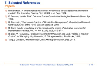
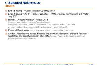

The document discusses prudent valuation in the context of global derivatives trading and risk management, focusing on its regulatory background and theoretical foundations. It highlights the need for financial institutions to apply prudent valuation in accordance with capital requirements, bridging the gap between fair value assessment and risk management practices. Key topics include valuation uncertainty, market incompleteness, and various valuation adjustments that impact core equity capital.


