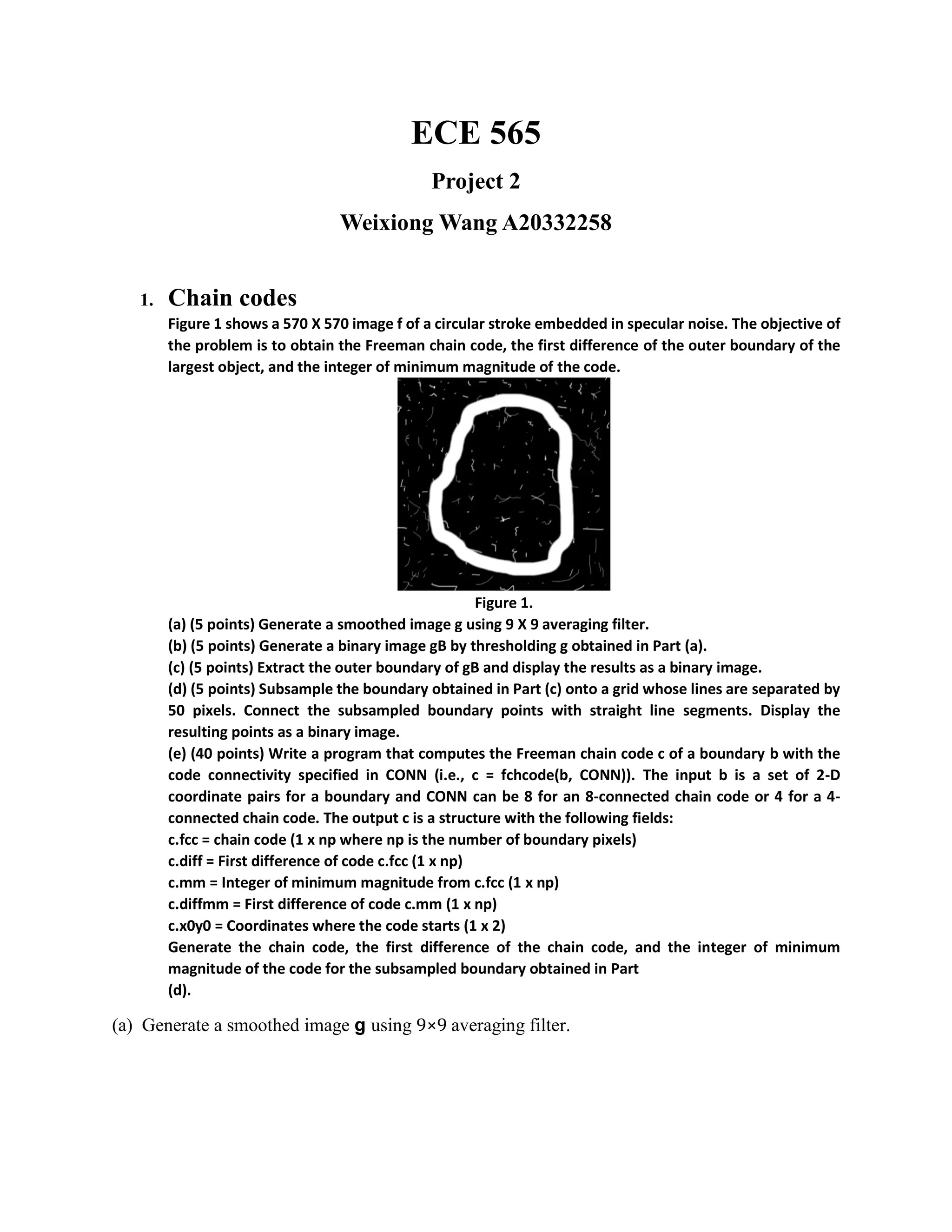
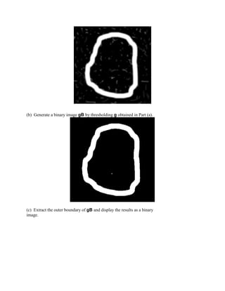
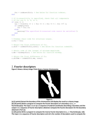
The document describes a project involving image processing and boundary analysis. It includes: 1. Smoothing an image, thresholding it to binary, extracting the outer boundary, subsampling the boundary, and computing the Freeman chain code and descriptors of the subsampled boundary. 2. Extracting the boundary of an image of a chromosome, computing the Fourier descriptors of the boundary, and reconstructing the boundary using different percentages of the descriptors. 3. The provided code computes Freeman chain codes, Fourier descriptors, and performs other boundary analysis tasks like subsampling and reconstruction from descriptors.

1. ECE 565
Project 2
Weixiong Wang A20332258
1. Chain codes
Figure 1 shows a 570 X 570 image f of a circular stroke embedded in specular noise. The objective of
the problem is to obtain the Freeman chain code, the first difference of the outer boundary of the
largest object, and the integer of minimum magnitude of the code.
Figure 1.
(a) (5 points) Generate a smoothed image g using 9 X 9 averaging filter.
(b) (5 points) Generate a binary image gB by thresholding g obtained in Part (a).
(c) (5 points) Extract the outer boundary of gB and display the results as a binary image.
(d) (5 points) Subsample the boundary obtained in Part (c) onto a grid whose lines are separated by
50 pixels. Connect the subsampled boundary points with straight line segments. Display the
resulting points as a binary image.
(e) (40 points) Write a program that computes the Freeman chain code c of a boundary b with the
code connectivity specified in CONN (i.e., c = fchcode(b, CONN)). The input b is a set of 2-D
coordinate pairs for a boundary and CONN can be 8 for an 8-connected chain code or 4 for a 4-
connected chain code. The output c is a structure with the following fields:
c.fcc = chain code (1 x np where np is the number of boundary pixels)
c.diff = First difference of code c.fcc (1 x np)
c.mm = Integer of minimum magnitude from c.fcc (1 x np)
c.diffmm = First difference of code c.mm (1 x np)
c.x0y0 = Coordinates where the code starts (1 x 2)
Generate the chain code, the first difference of the chain code, and the integer of minimum
magnitude of the code for the subsampled boundary obtained in Part
(d).
(a) Generate a smoothed image g using 9×9 averaging filter.

2. (b) Generate a binary image gB by thresholding g obtained in Part (a).
(c) Extract the outer boundary of gB and display the results as a binary
image.

3. (d) Subsample the boundary obtained in Part (c) onto a grid whose lines are
separated by 50 pixels. Connect the subsampled boundary points with straight line
segments. Display the resulting points as a binary image.
(e) Write a program that computes the Freeman chain code c of a boundary
b with the code connectivity specified in CONN (i.e., c = fchcode(b, CONN)).
The input b is a set of 2-D coordinate pairs for a boundary and CONN can be 8

4. for an 8-connected chain code or 4 for a 4-connected chain code. The output c is
a structure with the following fields.
chain code（1×32）：
c.fcc = 2220 2202 0000 6066 6666 6644 4444 2422
First difference of code c.fcc （1×32）：
c.diff = 0062 0626 0006 2600 0000 0600 0006 2600
Integer of minimum magnitude from c.fcc（1×32）：
c.mm = 0000 6066 6666 6644 4444 2422 2220 2202
First difference of code c.mm（1×32）：
c.diffmm = 0006 2600 0000 0600 0006 2600 0062 0626
Coordinates where the code starts（1×32）：
c.x0y0 = 83
Code:

5. f = imread('G:myimagesFigure1.tif');
imshow(f);
w=fspecial('average',9); % Set average filter as w.
g = imfilter(f,w,'symmetric'); % Smooth image.
figure
imshow(g,[])
level = graythresh(f); % Use O'tsu thresholding smoothed image.
BW = im2bw(g,level); % Binary image of g.
figure
imshow(BW)
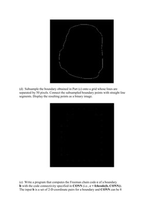
%Extract the outer boundary of gB and display the results as a binary image.
B=bwboundaries(BW);
d=cellfun('length',B);
[max_d,k]=max(d);
b=B{1};
[M,N]=size(BW);
g1=bound2im(b,M,N);
figure
imshow(g1)
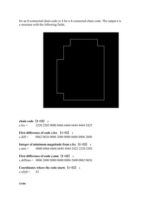
%Subsample the boundary
[s,su]=bsubsamp(b,50);
g2=bound2im(s,M,N);
figure
imshow(g2)
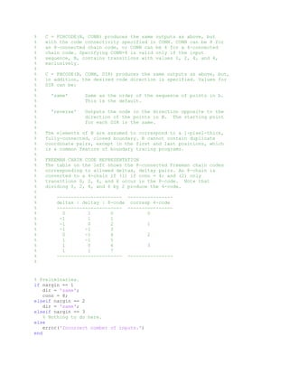
%Connect the subsampled boundary points with straight line segments.
cn=connectpoly(s(:,1),s(:,2));
g3=bound2im(cn,M,N);
figure
imshow(g3)
%computes the Freeman chain code c of a boundary b with the code connectivity
specified
%c.fcc c.diff c.mm c.diffmm c.x0y0
c=fchcode(su);
%%fchcode
function c = fchcode(b, conn, dir)
%FCHCODE Computes the Freeman chain code of a boundary.
% C = FCHCODE(B) computes the 8-connected Freeman chain code of a
% set of 2-D coordinate pairs contained in B, an np-by-2 array. C
% is a structure with the following fields:
%
% c.fcc = Freeman chain code (1-by-np)
% c.diff = First difference of code c.fcc (1-by-np)
% c.mm = Integer of minimum magnitude from c.fcc (1-by-np)
% c.diffmm = First difference of code c.mm (1-by-np)
% c.x0y0 = Coordinates where the code starts (1-by-2)
%

6. % C = FCHCODE(B, CONN) produces the same outputs as above, but
% with the code connectivity specified in CONN. CONN can be 8 for
% an 8-connected chain code, or CONN can be 4 for a 4-connected
% chain code. Specifying CONN=4 is valid only if the input
% sequence, B, contains transitions with values 0, 2, 4, and 6,
% exclusively.
%
% C = FHCODE(B, CONN, DIR) produces the same outputs as above, but,
% in addition, the desired code direction is specified. Values for
% DIR can be:
%
% 'same' Same as the order of the sequence of points in b.
% This is the default.
%
% 'reverse' Outputs the code in the direction opposite to the
% direction of the points in B. The starting point
% for each DIR is the same.
%
% The elements of B are assumed to correspond to a 1-pixel-thick,
% fully-connected, closed boundary. B cannot contain duplicate
% coordinate pairs, except in the first and last positions, which
% is a common feature of boundary tracing programs.
%
% FREEMAN CHAIN CODE REPRESENTATION
% The table on the left shows the 8-connected Freeman chain codes
% corresponding to allowed deltax, deltay pairs. An 8-chain is
% converted to a 4-chain if (1) if conn = 4; and (2) only
% transitions 0, 2, 4, and 6 occur in the 8-code. Note that
% dividing 0, 2, 4, and 6 by 2 produce the 4-code.
%
% ----------------------- ----------------
% deltax | deltay | 8-code corresp 4-code
% ----------------------- ----------------
% 0 1 0 0
% -1 1 1
% -1 0 2 1
% -1 -1 3
% 0 -1 4 2
% 1 -1 5
% 1 0 6 3
% 1 1 7
% ----------------------- ----------------
%
% Preliminaries.
if nargin == 1
dir = 'same';
conn = 8;
elseif nargin == 2
dir = 'same';
elseif nargin == 3
% Nothing to do here.
else
error('Incorrect number of inputs.')
end

7. [np, nc] = size(b);
if np < nc
error('B must be of size np-by-2.');
end
% Some boundary tracing programs, such as boundaries.m, output a
% sequence in which the coordinates of the first and last points are
% the same. If this is the case, eliminate the last point.
if isequal(b(1, :), b(np, :))
np = np - 1;
b = b(1:np, :);
end
% Build the code table using the single indices from the formula
% for z given above:
C(11)=0; C(7)=1; C(6)=2; C(5)=3; C(9)=4;
C(13)=5; C(14)=6; C(15)=7;
% End of Preliminaries.
% Begin processing.
x0 = b(1, 1);
y0 = b(1, 2);
c.x0y0 = [x0, y0];
% Make sure the coordinates are organized sequentially:
% Get the deltax and deltay between successive points in b. The
% last row of a is the first row of b.
a = circshift(b, [-1, 0]);
% DEL = a - b is an nr-by-2 matrix in which the rows contain the
% deltax and deltay between successive points in b. The two
% components in the kth row of matrix DEL are deltax and deltay
% between point (xk, yk) and (xk+1, yk+1). The last row of DEL
% contains the deltax and deltay between (xnr, ynr) and (x1, y1),
% (i.e., between the last and first points in b).
DEL = a - b;
% If the abs value of either (or both) components of a pair
% (deltax, deltay) is greater than 1, then by definition the curve
% is broken (or the points are out of order), and the program
% terminates.
if any(abs(DEL(:, 1)) > 1) | any(abs(DEL(:, 2)) > 1);
error('The input curve is broken or points are out of order.')
end
% Create a single index vector using the formula described above.
z = 4*(DEL(:, 1) + 2) + (DEL(:, 2) + 2);
% Use the index to map into the table. The following are
% the Freeman 8-chain codes, organized in a 1-by-np array.
fcc = C(z);
% Check if direction of code sequence needs to be reversed.
if strcmp(dir, 'reverse')

8. fcc = coderev(fcc); % See below for function coderev.
end
% If 4-connectivity is specified, check that all components
% of fcc are 0, 2, 4, or 6.
if conn == 4
val = find(fcc == 1 | fcc == 3 | fcc == 5 | fcc ==7 );
if isempty(val)
fcc = fcc./2;
else
warning('The specified 4-connected code cannot be satisfied.')
end
end
% Freeman chain code for structure output.
c.fcc = fcc;
% Obtain the first difference of fcc.
c.diff = codediff(fcc,conn); % See below for function codediff.
% Obtain code of the integer of minimum magnitude.
c.mm = minmag(fcc); % See below for function minmag.
% Obtain the first difference of fcc
c.diffmm = codediff(c.mm, conn);
2. Fourier descriptors
Figure 2 shows a binary image f that shows a human chromosome.
Figure 2.
(a) (2 points) Extract the boundary of the chromosome and display the result as a binary image.
(b) (18 points) Write a program to compute the Fourier descriptors of a boundary s (i.e., z =
fourierdescp(s)). The input s is an np x 2 sequence of ordered coordinates describing a boundary and the
output z is a sequence of Fourier descriptors obtained. Compute the Fourier descriptors for the boundary
obtained in Part (a).
(c) (20 points) Write a program to compute the inverse Fourier descriptors (i.e., s = ifourierdescp(z, nd)).
The input z is a sequence of Fourier descriptors and nd is the number of descriptors used to compute the

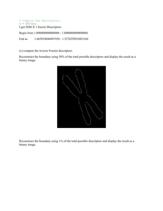
9. inverse. nd must be an even integer no greater than length(z). Reconstruct the boundary using 50% of the
total possible descriptors and display the result as a binary image. Then, reconstruct the boundary using
1% of the total possible descriptors and display the result as a binary image.
(a) Extract the boundary of the chromosome and display the result as a binary image.
(b) compute the Fourier descriptors of a boundary.(Below)
%%Fourier descriptor
function z = frdescp(s)
%FRDESCP Computes Fourier descriptors.
% Z = FRDESCP(S) computes the Fourier descriptors of S, which is an
% np-by-2 sequence of image coordinates describing a boundary.
%
% Preliminaries
[np, nc] = size(s);
if nc ~= 2
error('S must be of size np-by-2.');
end
if np/2 ~= round(np/2);
s(end + 1, :) = s(end, :);
np = np + 1;
end
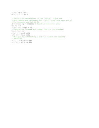
% Create an alternating sequence of 1s and -1s for use in centering
% the transform.
x = 0:(np - 1);
m = ((-1) .^ x)';
% Multiply the input sequence by alternating 1s and -1s to
% center the transform.
s(:, 1) = m .* s(:, 1);
s(:, 2) = m .* s(:, 2);
% Convert coordinates to complex numbers.
s = s(:, 1) + i*s(:, 2);

10. % Compute the descriptors.
z = fft(s);
I got 2688 X 1 fourier Descriptors.
Begin from 1.000000000000000 - 1.000000000000000i
End as 1.665834044491930 - 1.527629201082164i
(c) compute the inverse Fourier descriptors.
Reconstruct the boundary using 50% of the total possible descriptors and display the result as a
binary image.
Reconstruct the boundary using 1% of the total possible descriptors and display the result as a
binary image.

11. Conclusion:
The size of the figure, M=688, and N =540.length of the output in part_b is 2688. And the output is a
length(Z)-by-2 matrix containing the coordinates of a closed boundary.
We can find that under the 1%(which is 26) of the total possible descriptors, the obtained figure
distorted a lot than the original one, while it becomes smoother and the 50%(which is 1344) of the total
possible descriptors are nearly the same with the original one.
If we continuously decrease the number uintil 2 descriptors to reconstruct the figure, we will get a
circle .

12. Code:
f = imread('G:myimagesFigure2.tif');
%Extract the outer boundary of gB and display the results as a binary image.
B=bwboundaries(f);
d=cellfun('length',B);
[max_d,k]=max(d);
b=B{1};
[M,N]=size(f);
g1=bound2im(b,M,N);
figure
imshow(g1)
%Compute the fourier descriptor
z=frdescp(b);
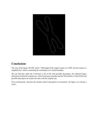
%Reconstruct the boundary using 50% of the total possible descriptors
z1344=ifrdescp(z,1344);
z1im1344=bound2im(z1344,M,N);
figure
imshow(z1im1344)
%Reconstruct the boundary using 1% of the total possible descriptors
z26=ifrdescp(z,26);
z1im26=bound2im(z26,M,N);
figure
imshow(z1im26)
%%Inverse Fourier descriptor
function s = ifrdescp(z, nd)
%IFRDESCP Computes inverse Fourier descriptors.
% S = IFRDESCP(Z, ND) computes the inverse Fourier descriptors of
% of Z, which is a sequence of Fourier descriptor obtained, for
% example, by using function FRDESCP. ND is the number of
% descriptors used to computing the inverse; ND must be an even
% integer no greater than length(Z). If ND is omitted, it defaults
% to length(Z). The output, S, is a length(Z)-by-2 matrix containing
% the coordinates of a closed boundary.
% Preliminaries.
np = length(z);
% Check inputs.
if nargin == 1 | nd > np
nd = np;
end
% Create an alternating sequence of 1s and -1s for use in centering
% the transform.

13. x = 0:(np - 1);
m = ((-1) .^ x)';
% Use only nd descriptors in the inverse. Since the
% descriptors are centered, (np - nd)/2 terms from each end of
% the sequence are set to 0.
d = round((np - nd)/2); % Round in case nd is odd.
z(1:d) = 0;
z(np - d + 1:np) = 0;
% Compute the inverse and convert back to coordinates.
zz = ifft(z);
s(:, 1) = real(zz);
s(:, 2) = imag(zz);
% Multiply by alternating 1 and -1s to undo the earlier
% centering.
s(:, 1) = m.*s(:, 1);
s(:, 2) = m.*s(:, 2);