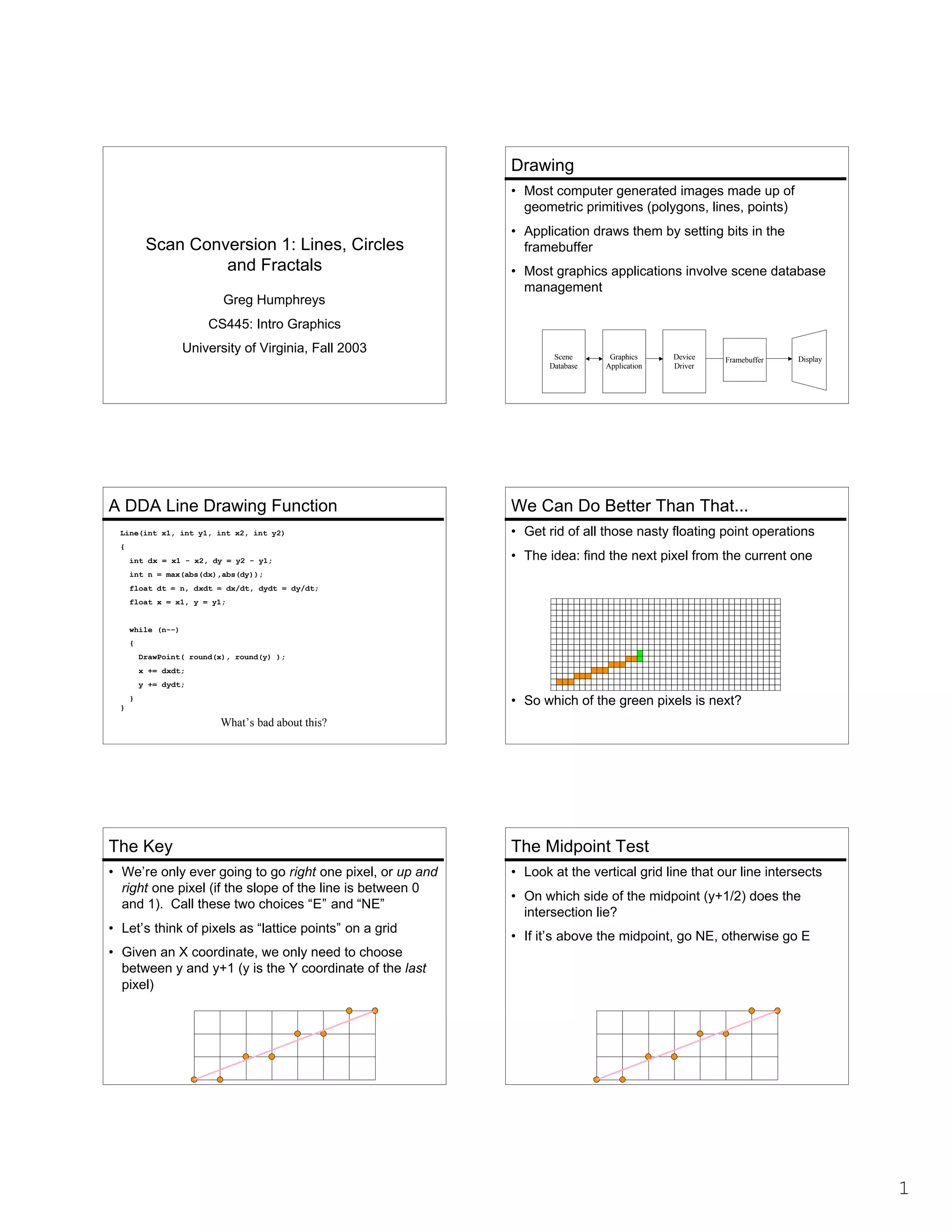
Drawing
• Most computer generated images made up of
geometric primitives (polygons, lines, points)

Scan Conversion 1: Lines, Circles
and Fractals
Greg Humphreys

• Application draws them by setting bits in the
framebuffer
• Most graphics applications involve scene database
management

CS445: Intro Graphics
University of Virginia, Fall 2003

A DDA Line Drawing Function
Line(int x1, int y1, int x2, int y2)
{
int dx = x1 - x2, dy = y2 - y1;

Scene
Database

Graphics
Application

Device
Driver

Framebuffer

Display

We Can Do Better Than That...
• Get rid of all those nasty floating point operations
• The idea: find the next pixel from the current one

int n = max(abs(dx),abs(dy));
float dt = n, dxdt = dx/dt, dydt = dy/dt;
float x = x1, y = y1;
while (n--)
{
DrawPoint( round(x), round(y) );
x += dxdt;
y += dydt;

• So which of the green pixels is next?

}
}

What’s bad about this?

The Key

The Midpoint Test

• We’re only ever going to go right one pixel, or up and
right one pixel (if the slope of the line is between 0
and 1). Call these two choices “E” and “NE”

• Look at the vertical grid line that our line intersects

• Let’s think of pixels as “lattice points” on a grid

• On which side of the midpoint (y+1/2) does the
intersection lie?
• If it’s above the midpoint, go NE, otherwise go E

• Given an X coordinate, we only need to choose
between y and y+1 (y is the Y coordinate of the last
pixel)

1
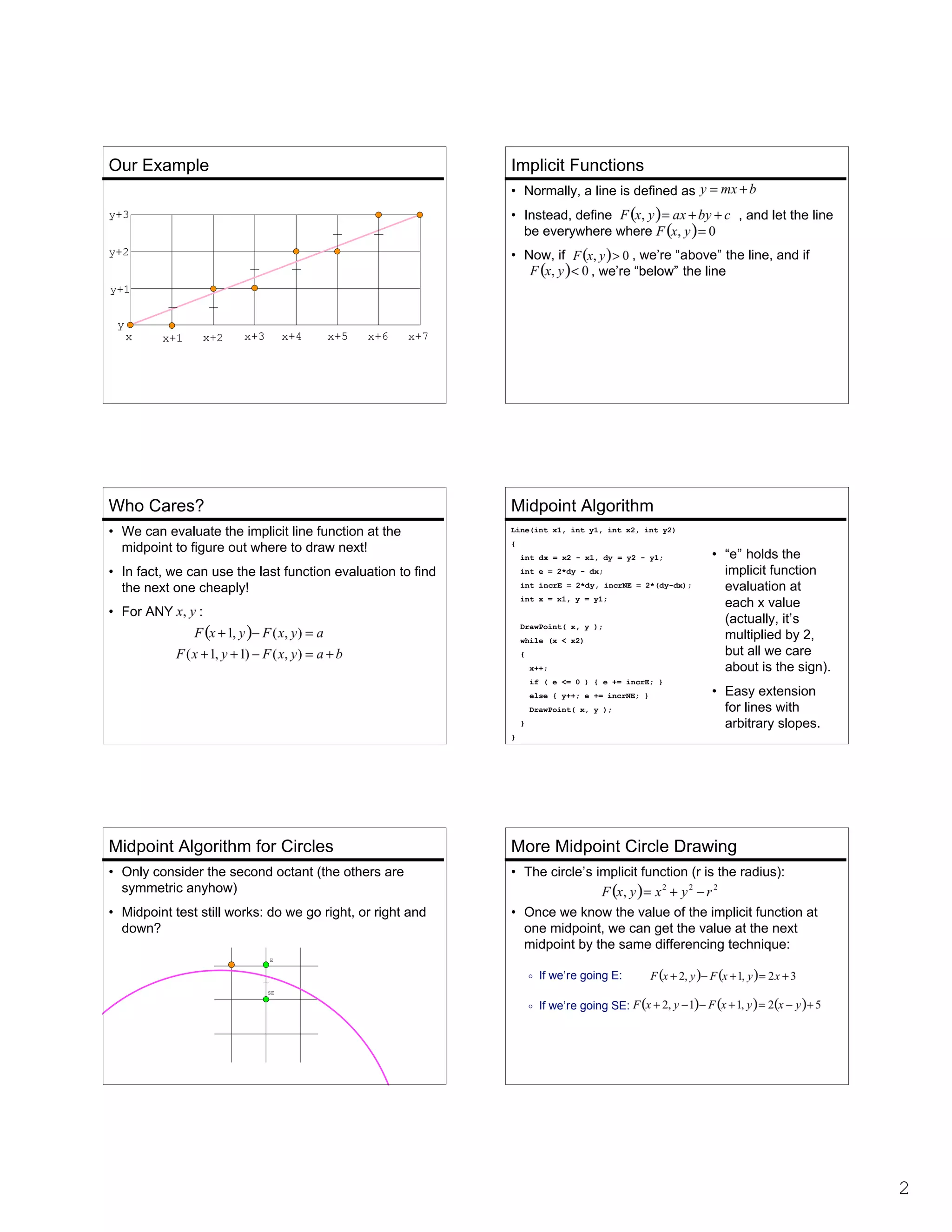
Our Example

Implicit Functions
• Normally, a line is defined as

y+3

• Instead, define
be everywhere where

y+2

• Now, if

, and let the line

, we’re “above” the line, and if
, we’re “below” the line

y+1
y

x

x+1

x+2

x+3

x+4

x+5

x+6

x+7

Who Cares?

Midpoint Algorithm

• We can evaluate the implicit line function at the
midpoint to figure out where to draw next!

Line(int x1, int y1, int x2, int y2)
{
int dx = x2 - x1, dy = y2 - y1;

• In fact, we can use the last function evaluation to find
the next one cheaply!
• For ANY

int e = 2*dy - dx;
int incrE = 2*dy, incrNE = 2*(dy-dx);
int x = x1, y = y1;

:
DrawPoint( x, y );
while (x < x2)
{
x++;
if ( e <= 0 ) { e += incrE; }
else { y++; e += incrNE; }
DrawPoint( x, y );
}

• “e” holds the
implicit function
evaluation at
each x value
(actually, it’s
multiplied by 2,
but all we care
about is the sign).
• Easy extension
for lines with
arbitrary slopes.

}

Midpoint Algorithm for Circles

More Midpoint Circle Drawing

• Only consider the second octant (the others are
symmetric anyhow)

• The circle’s implicit function (r is the radius):

• Midpoint test still works: do we go right, or right and
down?

• Once we know the value of the implicit function at
one midpoint, we can get the value at the next
midpoint by the same differencing technique:

E

 If we’re going E:
SE

 If we’re going SE:

2
Drawing the 2nd Octant

Final Circle Drawer

void Circle( int cx, int cy, int radius )
{
int x = 0, y = radius, e = 1-radius;
DrawPoint( x + cx, y + cy );

• Look at all those
expensive multiplies!
Can we get rid of them
too?

while (y > x)
{
if (e < 0) // Go “east”
{
e += 2*x + 3;
}
else // Go “south-east”
{
e += 2*(x-y) + 5;
y--;
}
x++;
DrawPoint( x + cx, y + cy );
}

void Circle( int
{
int x = 0, y =
int incrE = 3,
DrawPoint( x +

radius, e = 1-radius;
incrSE = -2*radius + 5
cx, y + cy );

while (y > x)
{
if (e < 0) // Go “east”
{
e += incrE;
incrE += 2; incrSE += 2;
}
else // Go “south-east”
{
e += incrSE;
incrE += 2; incrSE += 4;
y--;
}
x++;
DrawPoint( x + cx, y + cy );
}

• How about doing finite
differencing on the “e”
variable itself?
 If we go E:
 If we go SE:

}

cx, int cy, int radius )

This looks pretty fast!

}

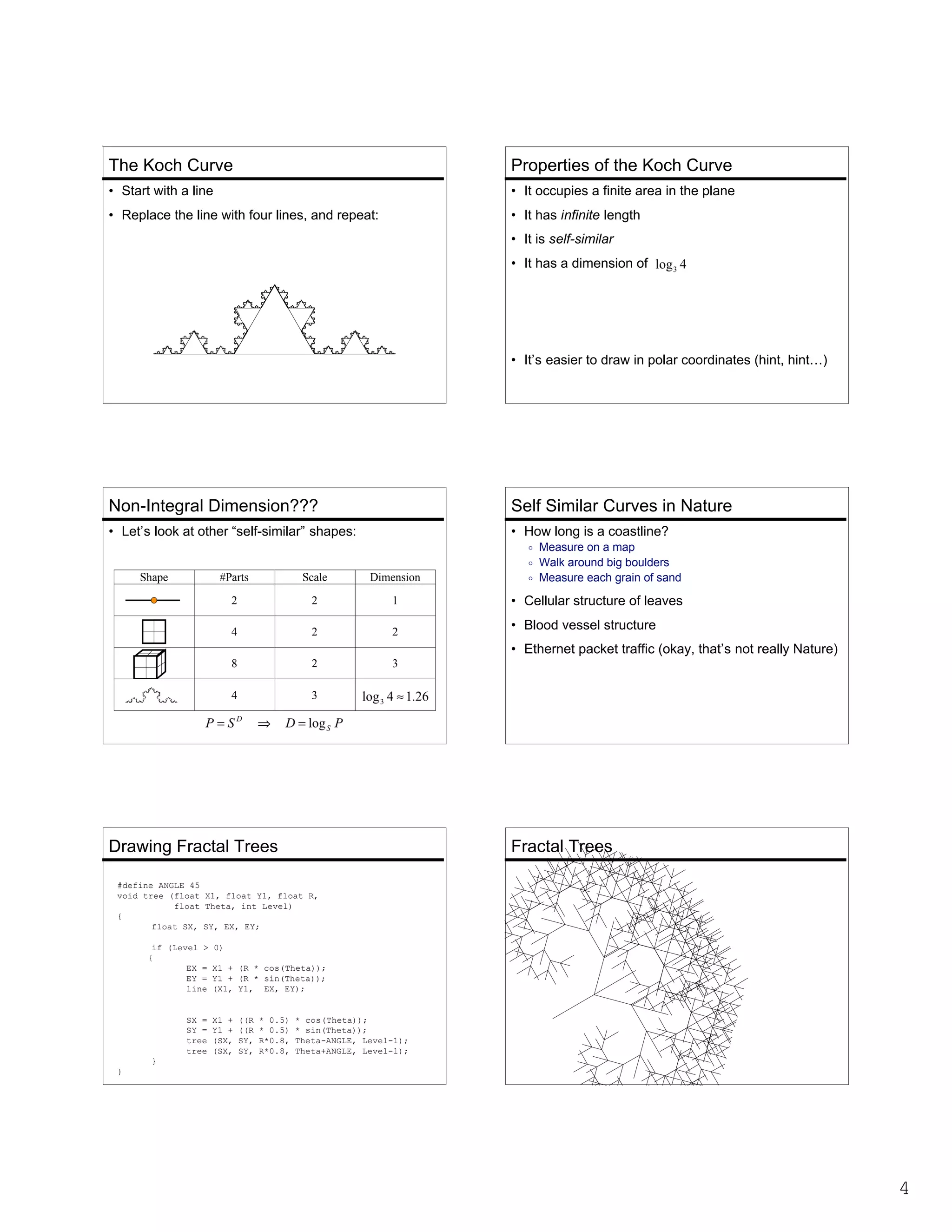
Flood Fill

Simple 4-connected Fill

• The idea: fill a “connected region” with a solid
color

• The simplest algorithm to fill a 4-connected region is
a recursive one:

• Term definitions:
8

4

8

4

1

4

8

4

8

• The center “1” pixel is 4-connected to the pixels
marked “4”, and 8-connected to the pixels
marked “8”

FloodFill( int x, int y, int inside_color, int new_color )
{
if (GetColor( x, y ) == inside_color)
{
SetColor( x, y, new_color );
FloodFill( x+1, y , inside_color, new_color );
FloodFill( x-1, y , inside_color, new_color );
FloodFill( x,
y+1, inside_color, new_color );
FloodFill( x,
y-1, inside_color, new_color );
}
}

A Span-based Algorithm

Fractals

• Definition: a run is a horizontal span of identically
colored pixels

• Fractal: any curve or shape exhibiting self-similarity
at any scale

h

b

c

s

a
d
e

f
g
i
Start at pixel “s”, the seed. Find the run containing “s” (“b”
to “a”). Fill that run with the new color. Then search every
pixel above that run, looking for other pixels of the interior
color. For each one found, find the right side of that run
(“c”), and push that on a stack. Do the same for the pixels
below (“d”). Then pop the stack and repeat the procedure
with the new seed. The algorithm finds runs ending at “e”,
“f”, “g”, “h”, and “i”

• Fractals appear in nature all the time
• Part of the general science of chaos

3
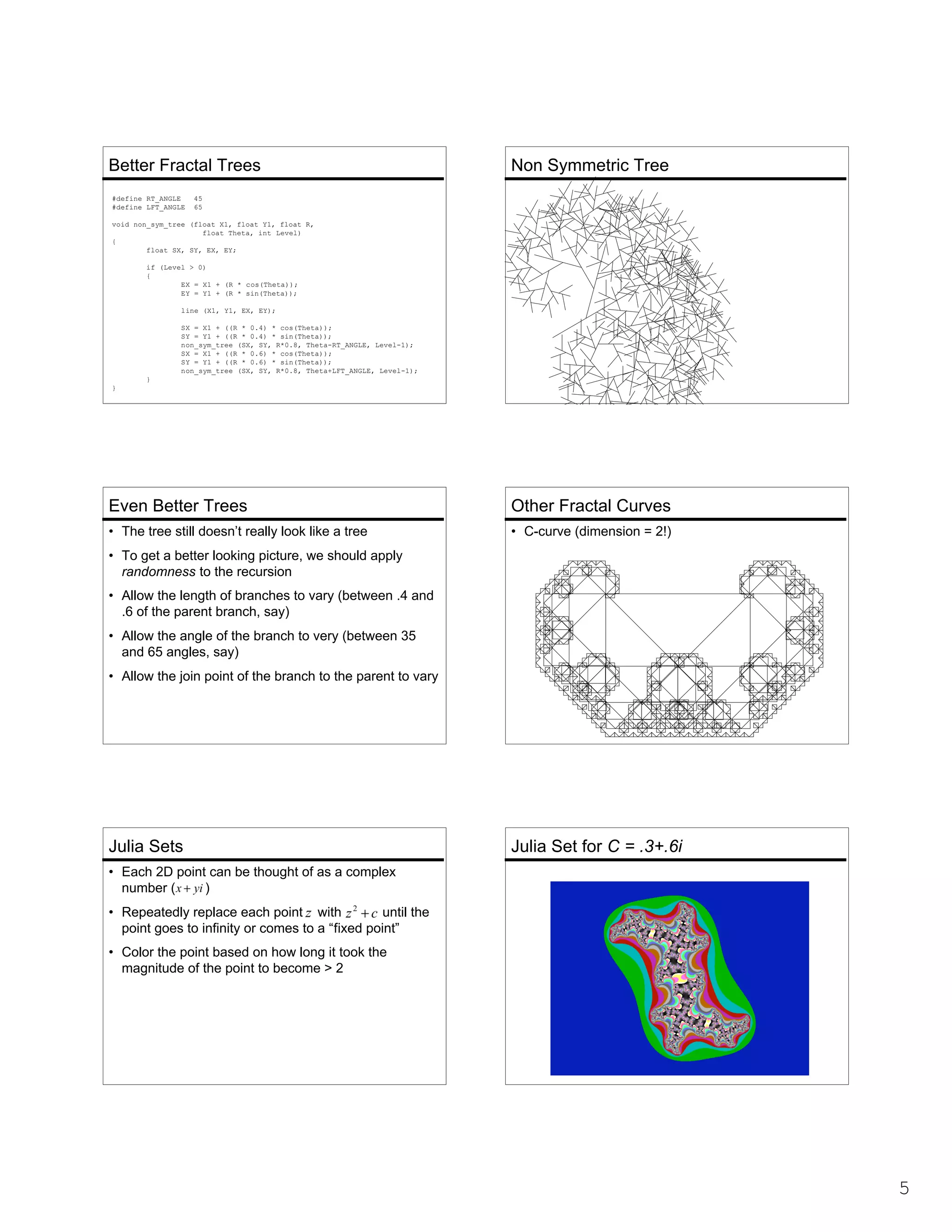
The Koch Curve

Properties of the Koch Curve

• Start with a line

• It occupies a finite area in the plane

• Replace the line with four lines, and repeat:

• It has infinite length
• It is self-similar
• It has a dimension of

• It’s easier to draw in polar coordinates (hint, hint…)

Non-Integral Dimension???

Self Similar Curves in Nature

• Let’s look at other “self-similar” shapes:

• How long is a coastline?

Shape

 Measure on a map
 Walk around big boulders
 Measure each grain of sand

#Parts

Scale

Dimension

2

2

1

• Cellular structure of leaves

4

2

2

• Blood vessel structure

8

2

3

4

3

?

• Ethernet packet traffic (okay, that’s not really Nature)

Drawing Fractal Trees

Fractal Trees

#define ANGLE 45
void tree (float X1, float Y1, float R,
float Theta, int Level)
{
float SX, SY, EX, EY;
if (Level >
{
EX =
EY =
line

SX =
SY =
tree
tree

0)
X1 + (R * cos(Theta));
Y1 + (R * sin(Theta));
(X1, Y1, EX, EY);

X1 +
Y1 +
(SX,
(SX,

((R
((R
SY,
SY,

* 0.5)
* 0.5)
R*0.8,
R*0.8,

* cos(Theta));
* sin(Theta));
Theta-ANGLE, Level-1);
Theta+ANGLE, Level-1);

}
}

4
Better Fractal Trees
#define RT_ANGLE
#define LFT_ANGLE

Non Symmetric Tree

45
65

void non_sym_tree (float X1, float Y1, float R,
float Theta, int Level)
{
float SX, SY, EX, EY;
if (Level > 0)
{
EX = X1 + (R * cos(Theta));
EY = Y1 + (R * sin(Theta));
line (X1, Y1, EX, EY);
SX = X1 + ((R * 0.4) * cos(Theta));
SY = Y1 + ((R * 0.4) * sin(Theta));
non_sym_tree (SX, SY, R*0.8, Theta-RT_ANGLE, Level-1);
SX = X1 + ((R * 0.6) * cos(Theta));
SY = Y1 + ((R * 0.6) * sin(Theta));
non_sym_tree (SX, SY, R*0.8, Theta+LFT_ANGLE, Level-1);
}
}

Even Better Trees

Other Fractal Curves

• The tree still doesn’t really look like a tree

• C-curve (dimension = 2!)

• To get a better looking picture, we should apply
randomness to the recursion
• Allow the length of branches to vary (between .4 and
.6 of the parent branch, say)
• Allow the angle of the branch to very (between 35
and 65 angles, say)
• Allow the join point of the branch to the parent to vary

Julia Sets

Julia Set for C = .3+.6i

• Each 2D point can be thought of as a complex
number (
)
• Repeatedly replace each point with
until the
point goes to infinity or comes to a “fixed point”
• Color the point based on how long it took the
magnitude of the point to become > 2

5
Julia Set for C = .2+.6i

Julia Set for C = .1+.6i

Mandelbrot Set

Assignment 4 Demo

• Almost like the Julia set, but use the original (x,y)
point instead of a constant c

6

10 linescan

  • 1.
    Drawing • Most computergenerated images made up of geometric primitives (polygons, lines, points) Scan Conversion 1: Lines, Circles and Fractals Greg Humphreys • Application draws them by setting bits in the framebuffer • Most graphics applications involve scene database management CS445: Intro Graphics University of Virginia, Fall 2003 A DDA Line Drawing Function Line(int x1, int y1, int x2, int y2) { int dx = x1 - x2, dy = y2 - y1; Scene Database Graphics Application Device Driver Framebuffer Display We Can Do Better Than That... • Get rid of all those nasty floating point operations • The idea: find the next pixel from the current one int n = max(abs(dx),abs(dy)); float dt = n, dxdt = dx/dt, dydt = dy/dt; float x = x1, y = y1; while (n--) { DrawPoint( round(x), round(y) ); x += dxdt; y += dydt; • So which of the green pixels is next? } } What’s bad about this? The Key The Midpoint Test • We’re only ever going to go right one pixel, or up and right one pixel (if the slope of the line is between 0 and 1). Call these two choices “E” and “NE” • Look at the vertical grid line that our line intersects • Let’s think of pixels as “lattice points” on a grid • On which side of the midpoint (y+1/2) does the intersection lie? • If it’s above the midpoint, go NE, otherwise go E • Given an X coordinate, we only need to choose between y and y+1 (y is the Y coordinate of the last pixel) 1
  • 2.
    Our Example Implicit Functions •Normally, a line is defined as y+3 • Instead, define be everywhere where y+2 • Now, if , and let the line , we’re “above” the line, and if , we’re “below” the line y+1 y x x+1 x+2 x+3 x+4 x+5 x+6 x+7 Who Cares? Midpoint Algorithm • We can evaluate the implicit line function at the midpoint to figure out where to draw next! Line(int x1, int y1, int x2, int y2) { int dx = x2 - x1, dy = y2 - y1; • In fact, we can use the last function evaluation to find the next one cheaply! • For ANY int e = 2*dy - dx; int incrE = 2*dy, incrNE = 2*(dy-dx); int x = x1, y = y1; : DrawPoint( x, y ); while (x < x2) { x++; if ( e <= 0 ) { e += incrE; } else { y++; e += incrNE; } DrawPoint( x, y ); } • “e” holds the implicit function evaluation at each x value (actually, it’s multiplied by 2, but all we care about is the sign). • Easy extension for lines with arbitrary slopes. } Midpoint Algorithm for Circles More Midpoint Circle Drawing • Only consider the second octant (the others are symmetric anyhow) • The circle’s implicit function (r is the radius): • Midpoint test still works: do we go right, or right and down? • Once we know the value of the implicit function at one midpoint, we can get the value at the next midpoint by the same differencing technique: E  If we’re going E: SE  If we’re going SE: 2
  • 3.
    Drawing the 2ndOctant Final Circle Drawer void Circle( int cx, int cy, int radius ) { int x = 0, y = radius, e = 1-radius; DrawPoint( x + cx, y + cy ); • Look at all those expensive multiplies! Can we get rid of them too? while (y > x) { if (e < 0) // Go “east” { e += 2*x + 3; } else // Go “south-east” { e += 2*(x-y) + 5; y--; } x++; DrawPoint( x + cx, y + cy ); } void Circle( int { int x = 0, y = int incrE = 3, DrawPoint( x + radius, e = 1-radius; incrSE = -2*radius + 5 cx, y + cy ); while (y > x) { if (e < 0) // Go “east” { e += incrE; incrE += 2; incrSE += 2; } else // Go “south-east” { e += incrSE; incrE += 2; incrSE += 4; y--; } x++; DrawPoint( x + cx, y + cy ); } • How about doing finite differencing on the “e” variable itself?  If we go E:  If we go SE: } cx, int cy, int radius ) This looks pretty fast! } Flood Fill Simple 4-connected Fill • The idea: fill a “connected region” with a solid color • The simplest algorithm to fill a 4-connected region is a recursive one: • Term definitions: 8 4 8 4 1 4 8 4 8 • The center “1” pixel is 4-connected to the pixels marked “4”, and 8-connected to the pixels marked “8” FloodFill( int x, int y, int inside_color, int new_color ) { if (GetColor( x, y ) == inside_color) { SetColor( x, y, new_color ); FloodFill( x+1, y , inside_color, new_color ); FloodFill( x-1, y , inside_color, new_color ); FloodFill( x, y+1, inside_color, new_color ); FloodFill( x, y-1, inside_color, new_color ); } } A Span-based Algorithm Fractals • Definition: a run is a horizontal span of identically colored pixels • Fractal: any curve or shape exhibiting self-similarity at any scale h b c s a d e f g i Start at pixel “s”, the seed. Find the run containing “s” (“b” to “a”). Fill that run with the new color. Then search every pixel above that run, looking for other pixels of the interior color. For each one found, find the right side of that run (“c”), and push that on a stack. Do the same for the pixels below (“d”). Then pop the stack and repeat the procedure with the new seed. The algorithm finds runs ending at “e”, “f”, “g”, “h”, and “i” • Fractals appear in nature all the time • Part of the general science of chaos 3
  • 4.
    The Koch Curve Propertiesof the Koch Curve • Start with a line • It occupies a finite area in the plane • Replace the line with four lines, and repeat: • It has infinite length • It is self-similar • It has a dimension of • It’s easier to draw in polar coordinates (hint, hint…) Non-Integral Dimension??? Self Similar Curves in Nature • Let’s look at other “self-similar” shapes: • How long is a coastline? Shape  Measure on a map  Walk around big boulders  Measure each grain of sand #Parts Scale Dimension 2 2 1 • Cellular structure of leaves 4 2 2 • Blood vessel structure 8 2 3 4 3 ? • Ethernet packet traffic (okay, that’s not really Nature) Drawing Fractal Trees Fractal Trees #define ANGLE 45 void tree (float X1, float Y1, float R, float Theta, int Level) { float SX, SY, EX, EY; if (Level > { EX = EY = line SX = SY = tree tree 0) X1 + (R * cos(Theta)); Y1 + (R * sin(Theta)); (X1, Y1, EX, EY); X1 + Y1 + (SX, (SX, ((R ((R SY, SY, * 0.5) * 0.5) R*0.8, R*0.8, * cos(Theta)); * sin(Theta)); Theta-ANGLE, Level-1); Theta+ANGLE, Level-1); } } 4
  • 5.
    Better Fractal Trees #defineRT_ANGLE #define LFT_ANGLE Non Symmetric Tree 45 65 void non_sym_tree (float X1, float Y1, float R, float Theta, int Level) { float SX, SY, EX, EY; if (Level > 0) { EX = X1 + (R * cos(Theta)); EY = Y1 + (R * sin(Theta)); line (X1, Y1, EX, EY); SX = X1 + ((R * 0.4) * cos(Theta)); SY = Y1 + ((R * 0.4) * sin(Theta)); non_sym_tree (SX, SY, R*0.8, Theta-RT_ANGLE, Level-1); SX = X1 + ((R * 0.6) * cos(Theta)); SY = Y1 + ((R * 0.6) * sin(Theta)); non_sym_tree (SX, SY, R*0.8, Theta+LFT_ANGLE, Level-1); } } Even Better Trees Other Fractal Curves • The tree still doesn’t really look like a tree • C-curve (dimension = 2!) • To get a better looking picture, we should apply randomness to the recursion • Allow the length of branches to vary (between .4 and .6 of the parent branch, say) • Allow the angle of the branch to very (between 35 and 65 angles, say) • Allow the join point of the branch to the parent to vary Julia Sets Julia Set for C = .3+.6i • Each 2D point can be thought of as a complex number ( ) • Repeatedly replace each point with until the point goes to infinity or comes to a “fixed point” • Color the point based on how long it took the magnitude of the point to become > 2 5
  • 6.
    Julia Set forC = .2+.6i Julia Set for C = .1+.6i Mandelbrot Set Assignment 4 Demo • Almost like the Julia set, but use the original (x,y) point instead of a constant c 6