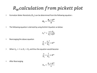
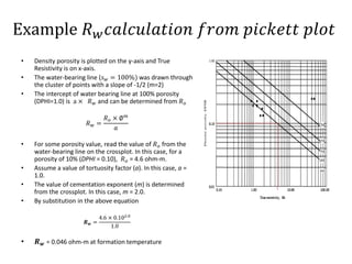
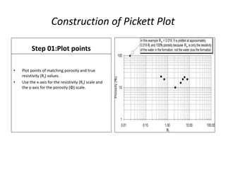
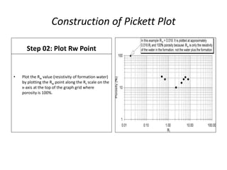
The Pickett plot is a graphical method derived from the Archie equation that visually represents true resistivity as a function of porosity and water saturation. It provides a means to estimate water saturation and formation water resistivity through the construction of a log-log plot, where true resistivity is plotted against porosity, allowing for analysis of different formation zones. While the technique has advantages in estimating water saturation without known prior parameters, it has limitations, such as difficulties with shaly formations and the assumption of constant formation lithology.

1. Pickett Plot

2. Pickett plot
• The Pickett plot is a visual representation of the Archie equation
• The Pickett method is on the observation that true resistivity (Rt) is a function of porosity, Water
saturation(Sw) and cementation exponent (m).
• The plot is named after G.R. Pickett.
• The plot is based on taking the logarithm of the Archie equation.
𝑅𝑡 =
𝑎 × 𝑅 𝑤
∅ 𝑚 × 𝑆 𝑤
𝑛
• Taking the logarithm of the equation produces:
log 𝑅𝑡 = log(𝑎 × 𝑅 𝑤)-mlog(∅) − 𝑛𝑙𝑜𝑔(𝑆 𝑤)
• If the zone is water bearing 𝑆 𝑤= 1, log 𝑆 𝑤 = 0 𝑎𝑛𝑑 𝑒𝑞𝑢𝑎𝑡𝑖𝑜𝑛 𝑟𝑒𝑑𝑢𝑐𝑒𝑠 𝑡𝑜
Log(𝑅𝑡) = log 𝑎 × 𝑅 𝑤 − 𝑚𝑙𝑜𝑔(∅)
• In practice (𝑅𝑡) is usually plotted on the x-axis and the porosity on the y-axis.
• This technique estimates water saturation and can also help determine
• Formation water Resistivity (𝑅 𝑤)
• Matrix parameter for sonic and density logs (∆𝑡 𝑚𝑎 & 𝜌 𝑚𝑎)

3. 𝑅 𝑤 𝑐𝑎𝑙𝑐𝑢𝑙𝑎𝑡𝑖𝑜𝑛 𝑓𝑟𝑜𝑚 𝑝𝑖𝑐𝑘𝑒𝑡𝑡 𝑝𝑙𝑜𝑡
• Formation Water Resistivity (𝑅 𝑤) can be determined from the following equation :
𝑹 𝒘 =
𝑹 𝒐 × ∅ 𝒎
𝒂
• The following equation is derived by using Archie’s Equation as below:
𝑆 𝑤
𝑛
=
𝑎 × 𝑅 𝑤
𝑅𝑡 × ∅ 𝑚
• Rearranging the above equation
𝑎
𝑅𝑡
=
𝑆 𝑤
𝑛
𝑅 𝑤
× ∅ 𝑚
• When 𝑆 𝑤 = 1 𝑠𝑜 𝑅𝑡 = 𝑅 𝑜 and thus the equation would become
𝑎
𝑅 𝑜
=
1
𝑅 𝑤
× ∅ 𝑚
• After Rearranging
𝑅 𝑤 =
𝑅 𝑜 × ∅ 𝑚
𝑎

4. Example 𝑅 𝑤 𝑐𝑎𝑙𝑐𝑢𝑙𝑎𝑡𝑖𝑜𝑛 𝑓𝑟𝑜𝑚 𝑝𝑖𝑐𝑘𝑒𝑡𝑡 𝑝𝑙𝑜𝑡
• Density porosity is plotted on the y-axis and True
Resistivity is on x-axis.
• The water-bearing line (𝑠 𝑤 = 100%) was drawn through
the cluster of points with a slope of -1/2 (m=2)
• The intercept of water bearing line at 100% porosity
(DPHI=1.0) is a × 𝑅 𝑤 and can be determined from 𝑅 𝑜
𝑅 𝑤 =
𝑅 𝑜 × ∅ 𝑚
𝑎
• For some porosity value, read the value of 𝑅 𝑜 from the
water-bearing line on the crossplot. In this case, for a
porosity of 10% (DPHI = 0.10), 𝑅 𝑜 = 4.6 ohm-m.
• Assume a value of tortuosity factor (a). In this case, a =
1.0.
• The value of cementation exponent (m) is determined
from the crossplot. In this case, m = 2.0.
• By substitution in the above equation
𝑹 𝒘 =
4.6 × 0.102.0
1.0
• 𝑹 𝒘 = 0.046 ohm-m at formation temperature

5. Construction of Pickett Plot
• Picket plot can be constructed if we have a value of Rw & m.
• The procedure for making a Pickett plot consists of five steps, detailed below.
1. Plot points of matching porosity and true resistivity (Rt ) on log-log paper.
2. Plot Rw point on the Rt scale.
3. Determine m using the table of values.
4. Plot the 100% Sw line.
5. Plot the lines representing lower values of Sw .
• These points are explained one by one for better understanding.

6. Construction of Pickett Plot
Step 01:Plot points
• Plot points of matching porosity and true
resistivity (Rt) values.
• Use the x-axis for the resistivity (Rt) scale and
the y-axis for the porosity (Φ) scale.

7. Construction of Pickett Plot
Step 02: Plot Rw Point
• Plot the Rw value (resistivity of formation water)
by plotting the Rw point along the Rt scale on the
x-axis at the top of the graph grid where
porosity is 100%.

8. Construction of Pickett Plot
Step 03:Determine m
• Estimate m (cementation factor) using the table
below.
Porosity Type Value of m
Sandstones with diagenetic or detrital clay in pores 1.7-1.8
Formations with clean, macro- to micro-sized pore
throat
2
Formations with vuggy porosity 2.2-3.0

9. Construction of Pickett Plot
Step 04:Plot the 100% Sw line
• On a pickett plot,the value of m determines the
slope of the S
• The first Sw line plotted on a Pickett plot is the
100% Sw line.
• To plot this line, draw a line with a negative
slope equal to m that begins at the Rw point.
• Use a linear scale to measure the slope; for
example, go down 1 in. and over 2 in.

10. Construction of Pickett Plot
Step 05:Plot sw lines
• After plotting the 100% Sw line, plot the lines
representing lower percentages of Sw using this
procedure:
• Find the intercept of Rt = 1 and the 100% Sw line
(made in the last procedure).
• From this intercept, draw a line parallel to the x-
axis across the plot. Any point on this line has
the same porosity.
• Where this line passes through Rt of 2, 4, 6, 8,
14, and 20, draw a series of lines parallel to the
100% Sw line.
• Points on these lines correspond to Sw of 71, 50,
41, 35, 27, and 22%. These percentages are
calculated from the Archie equation using m = 2
and n = 2 at Rt of 2, 4, 6, 8, 14, and 20.

11. Advantages of Pickett Plot
• Water saturation can be predicted without prior knowledge of Rw, a, or m.
• Rw is directly predicted (if tortuosity factor (a) is known or estimated) from the intercept of the water
bearingline at a porosity of 1 (porosity = 100%)
• The advantage of Picket Plot is that similar water saturation values will plot a straight line even if the
porosity and resistivity values vary.
• This allows one to easily separate the formation into zones based on their calculated water saturation or in
gas saturation
• Picket Plot is better because it is good for low porosity formation where small variation of m cause large
variations in Sw.

12. Limitations of Pickett Plot
• One of the weaknesses of the Pickett plot is its inability to handle shaly formation
• Values for pma and ∆tma must be assumed (although in cases with a wide range of porosities in the water
bearing zone.
• A wide range of porosity must be present to positively determine a water-bearing line.
• Formation lithology and water resistivity must be constant over the intervals compared in the plot.

13. Distinguish between Pay zone & Water Leg
• The Pickett plot can be illustrated with the
hypothetical data set of resistivity and porosity
values logged, with “Archie rock” properties and
a simple reservoir profile
• The example consists of a pay section at
irreducible water saturation (zones A-E), a
transition zone (Zone F), above a water leg (zones
G-J).

14. Distinguish between Pay zone & Water Leg
• Zones A to E have much higher resistivities
than zones H to J, even though they have
similar porosities, and suggests that these
zones may have appreciable hydrocarbon
content.
• Zone F is intermediate between these two
clusters, and its depth relationship to them
indicates that it may be in a transition zone.
• The zone H-J trend of a systematic decline in
resistivity with porosity also favors their
interpretation as possible water zones.

15. References
• Basic Well Log Analysis (2nd Edition) By George Asquith & Daniel Krygowski
• http://wiki.aapg.org/Pickett_plot_construction
• http://www.glossary.oilfield.slb.com/Terms/p/pickett_plot.aspx
• http://www.kgs.ku.edu/software/PfEFFER-java/HELP/PfEFFER/Pfeffer-theory3.html