openheim chapter 3 frequncy

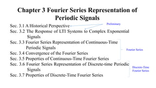
1. Chapter 3 Fourier Series Representation of
Periodic Signals
Sec. 3.1 A Historical Perspective
Sec. 3.2 The Response of LTI Systems to Complex Exponential
Signals
Sec. 3.3 Fourier Series Representation of Continuous-Time
Periodic Signals
Sec. 3.4 Convergence of the Fourier Series
Sec. 3.5 Properties of Continuous-Time Fourier Series
Sec. 3.6 Fourier Series Representation of Discrete-time Periodic
Signals
Sec. 3.7 Properties of Discrete-Time Fourier Series
Fourier Series
Discrete-Time
Fourier Series
Preliminary

2. Sec. 3.8 Fourier Series and LTI Systems
Sec. 3.9 Filtering
Sec. 3.10 Examples of Continuous-time Filters Described by
Differential Equations
Sec. 3.11 Examples of Discrete-time Filters Described by
Difference Equations
Sec. 3.12 Summary
Chapter 3 Fourier Series Representation of
Periodic Signals
LTI System
Analysis by
Discrete /
Continuous Time
Fourier Series
This section can be divided into 4 parts.

3. Fourier
Family
Continuous
Discrete
Periodic
Non-periodic Fourier Transform (Chap. 4)
Fourier Series (Chap. 3)
Periodic
Non-periodic Discrete-Time Fourier
Transform (Chap. 5)
Discrete-time Fourier
Series (Discrete Fourier
Transform) (Sec. 3.6)

4. Sec. 3.1 A Historical Perspective
L. Euler’s study
on the motion of a
vibrating string in
1748
P.203

5. In 1807, Jean Baptiste Joseph Fourier
Submitted a paper of using trigonometric series to represent “any” periodic signal
D. Bernoulli argued (in 1753)
All physical motions of a string could be represented by linear combinations of
normal modes
J.L. Lagrange strongly criticized (in 1759)
The use of trigonometric series in examination of vibrating strings
In 1822, Fourier published a book , “Theorie analytique de la chaleur”
“The Analytical Theory of Heat”
P.203

6. Fourier’s main contributions:
Studied vibration, heat diffusion, etc.
Found series of harmonically related sinusoids to be useful in
representing the temperature distribution through a body
Claimed that “any” periodic signal could be represented by such a
series (i.e., Fourier series discussed in Chap 3)
Obtained a representation for aperiodic signals (i.e., Fourier integral or
transform discussed in Chap 4 & 5)
(Fourier did not actually contribute to the mathematical theory of
Fourier series)
P.204

7. Impact from Fourier’s work:
Theory of integration, point-set topology, eigenfunction expansions,
etc.
Motion of planets, periodic behavior of the earth’s climate, wave in
the ocean, radio & television stations
Harmonic time series in the 18th & 19th centuries
Gauss etc. on discrete-time signals and systems
Faster Fourier transform (FFT) in the mid-1960s
Cooley (IBM) & Tukey (Princeton) reinvented in 1965
Can be found in Gauss’s notebooks (in 1805)

8. Sec. 3.2 The Response of LTI Systems to Complex Exponential
Signals
Key concept
The functions exp(st) and zn are the eigenfunctions of continuous-time and discrete-
time LTI systems, respectively
The basic signals exp(st) and zn has the following properties
1. The set of basic signals can be used to construct a broad and useful class of signals.
2. The response of an LTI system to each signal should be simple enough in structure to
provide us with a convenient representation for the response of the system to any signal
constructed as a linear combination of the basic signals.
P.206

9. Theorem 3.1 Eigenfunctions of LTI Systems
The functions exp(st) and zn are the eigenfunctions of continuous-time and discrete-
time LTI systems, respectively.
continuous time: est → H(s)est
discrete time: zn → H(z)zn
H(s) and H(z) are eigenvalues (may be complex)
P.206

10. with x(t) = est
(Proof):
( )
( ) ( ) ( ) ( ) .
s t
y t h x t d h e d

    
 

 
  
 
 
( ) ( )
st s st
y t e h e d H s e

 



 

  ( ) s
H s h e d

 



 
where
(Linear Combination):
1 1
2 2
3 3
1 1 1
2 2 2
3 3 3
( ) ,
( ) ,
( ) ,
s t s t
s t s t
s t s t
a e a H s e
a e a H s e
a e a H s e



3 3
1 2 1 2
1 2 3 1 1 2 2 3 3
( ) ( ) ( )
s t s t
s t s t s t s t
a e a e a e a H s e a H s e a H s e
    
P.207-208

11. [Example 3.1]
( ) ( 3)
y t x t
 
(1) When x(t) = ej2t
2( 3) 6 2
( ) j t j j t
y t e e e
 
 
3
( ) ( 3) s s
H s e d e

  

 

  

eigenvalue: 6
j
e
eigenvalue for est
is an LTI system with the impulse response  (t-3).
P.209
6
( 2) j
H j e

so that

12. [Example 3.1]
( ) ( 3)
y t x t
  is an LTI system with the impulse response  (t-3).
3
( ) ( 3) s s
H s e d e

  

 

  

eigenvalue for est
(2) When x(t) = cos(4t) + cos(7t).
4 4 7 7
1 1 1 1
2 2 2 2
( ) j t j t j t j t
x t e e e e
 
   
12 4 12 4 21 7 21 7
1 1 1 1
2 2 2 2
( ) j j t j j t j j t j j t
y t e e e e e e e e
   
   
( ) cos(4( 3)) cos(7( 3))
y t t t
   
P.209-210
4( 3) 4( 3) 7( 3) 7( 3)
1 1 1 1
2 2 2 2
( ) j t j t j t j t
y t e e e e
     
   

13. Sec. 3.3 Fourier Series Representation of Continuous-Time
Periodic Signals
Key concepts
(i) definition of the Fourier series;
(ii) how to apply the Fourier series to periodic signals
P.210

14. 3.3.1 Linear Combinations of Harmonically Related Complex Exponential
Signals
exp(st): eigenfunctions of continuous-time LTI systems
s can be complex.
If
( ) ( )
x t x t T
 
express it as
0 (2 / )
( ) jk t jk T t
k k
k k
x t a e a e
 
 
 
 
 
(2 / )
jk T t
e 
are eigenfunctions of continuous-time LTI systems
P.210-211

15. P.211

16. [Example 3.2]
P.211-212

17. [Example 3.2]
P.212

18. 0
( ) jk t
k
k
x t a e 


 
If x(t) is real
0 0
* *
( ) ( ) jk t jk t
k k
k k
x t x t a e a e
 
 



 
  
 
*
k k
a a

0 0
*
0
1
( ) [ ]
jk t jk t
k k
k
x t a a e a e
 



  

Therefore,
0
0
1
( ) 2 { }
jk t
k
k
x t a e a e 


  

P.213

19. 0 0
0
1
( ) 2 { }
jk t jk t
k k
k k
x t a e a e a e
 
 
 
   
 
(1) If
(2) If
P.214
k
j
k k
a A e 

0
0
1
0 0
1
( ) 2 { }
2 cos( )
k
j jk t
k
k
k k
k
x t a e A e e
a A k t
 
 




  
  


k k k
a B jC
 
 
0 0 0
1
( ) 2 cos sin
k k
k
x t a B k t C k t
 


  


20. 3.3.2 Determination of the Fourier Series Representation of a Continuous-
Time Periodic Signal
0 (2 / )
( ) jk t jk T t
k k
k k
x t a e a e
 
 
 
 
  How do we find ak?
0 0 0
( ) jn t jk t jn t
k
k
x t e a e e
  

 

 
0 0 0 0
( )
0 0 0
( )
T T T
jn t jk t jn t j k n t
k k
k k
x t e dt a e e dt a e dt
   
 
  
 
 
 
 
 
 
  
P.214

21. 0 0
( ) ( )
0
0
0
1
0
( )
T T
j k n t j k n t
e dt e
j k n
 

 
 

 0
2
T

 
Therefore,
When k  n
0
( )
0
,
0,
T
j k n t T k n
e dt
k n

 

 



0 0
( )
0 0
( )
T T
jn t j k n t
k n
k
x t e dt a e dt Ta
 

 

 
 
 
 

 
0
0
1
( )
T
jn t
n
a x t e dt
T


 
P.215

22. Definition 3.1 Fourier Series
for a continuous and periodic signal x(t) = x(t+T)
synthesis: 0 (2 / )
( ) jk t jk T t
k k
k k
x t a e a e
 
 
 
 
 
analysis: 0 (2 / )
1 1
( ) ( )
jk t jk T t
k
T T
a x t e dt x t e dt
T T
 
 
 
 
T
 is the integration from t0 to t0+T and t0 can be any value
Specially, if t0 = 0,
analysis: 0 (2 / )
0 0
1 1
( ) ( )
T T
jk t jk T t
k
a x t e dt x t e dt
T T
 
 
 
 
P.216

23. analysis: 0 (2 / )
1 1
( ) ( )
jk t jk T t
k
T T
a x t e dt x t e dt
T T
 
 
 
 
{ak} are often called the Fourier series coefficients or the spectral coefficients of x(t).
Specially, when k = 0,
0
1
( )
T
a x t dt
T
 
P.216

24. Supplement: Alternative Forms of the Fourier Series
0
2
( ) j k f t
k
k
x t a e 


 
synthesis:
analysis:
0
2
1
( ) j k f t
k
T
a x t e dt
T


  where f0 = 1/T.
synthesis:
analysis:
0
1
( ) jk t
k
k
x t a e
T




 
0
1 ( ) jk t
k
T
a x t e dt
T

 

25. [Example 3.3]
0 0
0
1 1
( ) sin .
2 2
j t j t
x t t e e
j j
 
 
  
0
( ) jk t
k
k
x t a e 


 
1 1
1 1
, , 0. 1 1.
2 2
k
a a a k or
j j

      
P.217

26. [Example 3.4]
0
( ) jk t
k
k
x t a e 


 
 
0 0 0 0 0 0
0 0 0 0
0 0 0
(2 /4) (2 /4)
2 2
( /4) ( /4)
( ) 1 sin 2cos cos 2 / 4 ,
1 1
( ) 1 [ ] [ ] [ ].
2 2
1 1 1 1
1 1 1 .
2 2 2 2
j t j t j t j t j t j t
j t j t j t j t
j j
x t t t t
x t e e e e e e
j
e e e e e e
j j
       
   
 
   
    
 

    
      
       
      
   
   
   
   
0
1
1
1
1 1
1 1
2 2
1 1
1 1
2 2
a
a j
j
a j
j


 
   
 
 
 
   
 
 
( /4)
2
( /4)
2
2
1 (1 )
2 4
2
1 (1 )
2 4
0, 2
j
j
k
a e j
a e j
a k




  
  
 
P.217-218

27. 0
1
1
1
1 1
1 1
2 2
1 1
1 1
2 2
a
a j
j
a j
j


 
   
 
 
 
   
 
 
( /4)
2
( /4)
2
2
1 (1 )
2 4
2
1 (1 )
2 4
0, 2
j
j
k
a e j
a e j
a k




  
  
 
P.218

28. [Example 3.5]
0
( ) jk t
k
k
x t a e 


 
1
1
1,
( )
0, / 2
t T
x t
T t T
 

 
 


1
1
1
0
2
1 T
T
T
a dt
T T

 

1
0 0 1
1
1
0 1 0 1
0
0 1
0
1 1
sin( )
2
, 0
2
T
jk t jk t T
k T
T
jk T jk T
a e dt e
T jk T
k T
e e
k
k T j k
 
 


 
 



  
 

  
 
 

P.218-219

29. 1
0
2T
a
T
 0 1
sin( )
k
k T
a
k



T = 4T1
T = 8T1
T = 16T1
P.220