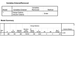
REGRESI KELOMPOK 4: ARMAN FERNANDO. S DETTI APRIANI ENI INDRIATI
DEFINISI REGRESI #  Menurut Sir Francis Galton (1822-1911)  Persamaan Regresi :Persamaan matematik yang memungkinkan peramalan nilai suatu peubah takbebas ( dependent variable ) dari nilai peubah bebas (independent variable). Jenis-jenis Persamaan Regresi :  Regresi Linier :  Regresi Linier Sederhana & Regresi Linier Berganda  Regresi Nonlinier Regresi Eksponensial - Bentuk Umum Regresi Linier Sederhana  Y = a + bX  Y : peubah takbebas  X : peubah bebas  a : konstanta  b : kemiringan
 
 
Data hasil pengamatan Regresi ∑ y= 306 ∑ x2= 555 ∑ x1= 183     68 125 38 T 6 60 100 33 S 5 40 90 29 R 4 55 85 28 Q 3 47 85 28 P 2 36 70 27 O 1 Berat Badan Harga Celana (puluh ribuan) Ukuran Celana NAMA NO.
Regression Descriptive Statistics 6 18.64135 92.5000 Harga Celana 6 4.23084 30.5000 Ukuran Celana 6 12.23111 51.0000 Berat Badan N Std. Deviation Mean
Variables Entered/Removed Model Summary Enter . Harga Celana, Ukuran Celana 1 Method Variables Removed Variables Entered Model 3.248 Durbin-Watson .127 3 2 4.445 .748 7.93132 .580 .748 .865 1 Sig. F Change df2 df1 F Change R Square Change Change Statistics Std. Error of the Estimate Adjusted R Square R Square R Model
 
Residuals Statistics 6 .254 .333 .690 .168 Centered Leverage Value 6 .662 .460 1.784 .001 Cook's Distance 6 1.270 1.667 3.451 .842 Mahal. Distance 6 1.289 -.163 1.694 -2.059 Stud. Deleted Residual 6 12.53070 -3.5050 12.9319 -19.8228 Deleted Residual 6 1.028 -.118 1.329 -1.428 Stud. Residual 6 .775 .000 1.084 -1.159 Std. Residual 6 6.14357 .0000 8.5978 -9.1957 Residual 6 11.64868 54.5050 75.7143 42.0681 Adjusted Predicted Value 6 1.35073 5.47106 7.34186 4.59157 Standard Error of Predicted Value 6 1.000 .000 1.755 -1.150 Std. Predicted Value 6 10.57622 51.0000 69.5652 38.8370 Predicted Value N Std. Deviation Mean Maximum Minimum
Charts
 
∑ Y²= 16354 ∑ (X2)²= 53075 ∑ (x1)²= 5671 ∑ x2= 29290 ∑ x1y= 9552 ∑ y= 306 ∑ x2= 555 ∑ x1= 183     4624 15625 1444 8500 2584 68 125 38 T 6 3600 10000 1089 6000 1980 60 100 33 S 5 1600 8100 841 3600 1160 40 90 29 R 4 3025 7225 784 4675 1540 55 85 28 Q 3 2209 7225 784 3995 1316 47 85 28 P 2 1296 4900 729 2520 972 36 70 27 O 1 Y² (X2)² (x1)² x2y x1y Y x2 x1 NAMA NO.
b=  (6 X 9552) - (183)(306) (6 X 5671) - (183)² =  1314 537 = 2,44 a= (306:6) – (2,44 X (183 : 6)) = 51 – (- 23,42) = 51+ 23,42 = 74,42 Y= 74,42 + 2,44x
b=  (6 X 29290) - (555)(306) (6 X 53075) - (555) =  5910 10425 = 0, 566 a= (306:6) – (0,566 X (555 : 6))  = 51 – (52,355) = -1,355 Y= 0,566 – 1,355x

Pp Regresi. Jadippt

  • 1.
    REGRESI KELOMPOK 4:ARMAN FERNANDO. S DETTI APRIANI ENI INDRIATI
  • 2.
    DEFINISI REGRESI # Menurut Sir Francis Galton (1822-1911) Persamaan Regresi :Persamaan matematik yang memungkinkan peramalan nilai suatu peubah takbebas ( dependent variable ) dari nilai peubah bebas (independent variable). Jenis-jenis Persamaan Regresi : Regresi Linier : Regresi Linier Sederhana & Regresi Linier Berganda Regresi Nonlinier Regresi Eksponensial - Bentuk Umum Regresi Linier Sederhana Y = a + bX Y : peubah takbebas X : peubah bebas a : konstanta b : kemiringan
  • 3.
  • 4.
  • 5.
    Data hasil pengamatanRegresi ∑ y= 306 ∑ x2= 555 ∑ x1= 183     68 125 38 T 6 60 100 33 S 5 40 90 29 R 4 55 85 28 Q 3 47 85 28 P 2 36 70 27 O 1 Berat Badan Harga Celana (puluh ribuan) Ukuran Celana NAMA NO.
  • 6.
    Regression Descriptive Statistics6 18.64135 92.5000 Harga Celana 6 4.23084 30.5000 Ukuran Celana 6 12.23111 51.0000 Berat Badan N Std. Deviation Mean
  • 7.
    Variables Entered/Removed ModelSummary Enter . Harga Celana, Ukuran Celana 1 Method Variables Removed Variables Entered Model 3.248 Durbin-Watson .127 3 2 4.445 .748 7.93132 .580 .748 .865 1 Sig. F Change df2 df1 F Change R Square Change Change Statistics Std. Error of the Estimate Adjusted R Square R Square R Model
  • 8.
  • 9.
    Residuals Statistics 6.254 .333 .690 .168 Centered Leverage Value 6 .662 .460 1.784 .001 Cook's Distance 6 1.270 1.667 3.451 .842 Mahal. Distance 6 1.289 -.163 1.694 -2.059 Stud. Deleted Residual 6 12.53070 -3.5050 12.9319 -19.8228 Deleted Residual 6 1.028 -.118 1.329 -1.428 Stud. Residual 6 .775 .000 1.084 -1.159 Std. Residual 6 6.14357 .0000 8.5978 -9.1957 Residual 6 11.64868 54.5050 75.7143 42.0681 Adjusted Predicted Value 6 1.35073 5.47106 7.34186 4.59157 Standard Error of Predicted Value 6 1.000 .000 1.755 -1.150 Std. Predicted Value 6 10.57622 51.0000 69.5652 38.8370 Predicted Value N Std. Deviation Mean Maximum Minimum
  • 10.
  • 11.
  • 12.
    ∑ Y²= 16354∑ (X2)²= 53075 ∑ (x1)²= 5671 ∑ x2= 29290 ∑ x1y= 9552 ∑ y= 306 ∑ x2= 555 ∑ x1= 183     4624 15625 1444 8500 2584 68 125 38 T 6 3600 10000 1089 6000 1980 60 100 33 S 5 1600 8100 841 3600 1160 40 90 29 R 4 3025 7225 784 4675 1540 55 85 28 Q 3 2209 7225 784 3995 1316 47 85 28 P 2 1296 4900 729 2520 972 36 70 27 O 1 Y² (X2)² (x1)² x2y x1y Y x2 x1 NAMA NO.
  • 13.
    b= (6X 9552) - (183)(306) (6 X 5671) - (183)² = 1314 537 = 2,44 a= (306:6) – (2,44 X (183 : 6)) = 51 – (- 23,42) = 51+ 23,42 = 74,42 Y= 74,42 + 2,44x
  • 14.
    b= (6X 29290) - (555)(306) (6 X 53075) - (555) = 5910 10425 = 0, 566 a= (306:6) – (0,566 X (555 : 6)) = 51 – (52,355) = -1,355 Y= 0,566 – 1,355x