Physics 101 Lab ManualDr. W.A.AtkinsonSouthern Illinois .docx

Physics 101 Lab Manual
Dr. W.A.Atkinson
Southern Illinois University, Carbondale
Physics Department
Updated by Dr. Foudil Latioui
January 23, 2012
ii
1
1Copyright c!,2002, 2003 by William Atkinson. All rights
reserved. Permission is granted for students registered in
Physics
101 at Southern Illinois University to print this manual for
personal use. Reproductions for other purposes are not
permitted.
Contents
How to Write Labs vii
-1.1 What You Need to Bring to the Lab . . . . . . . . . . . . . . . . .
. . . . . . . . . . . . . . . vii
-1.2 The Pre-Lab . . . . . . . . . . . . . . . . . . . . . . . . . . . . . . . . . .
. . . . . . . . . . . vii

-1.3 Structure of the Labs . . . . . . . . . . . . . . . . . . . . . . . . . . . .
. . . . . . . . . . . . . vii
-1.4 How to Draw Graphs . . . . . . . . . . . . . . . . . . . . . . . . . . . .
. . . . . . . . . . . . . viii
0 Pre-Lab Questions 1
0.1 Pre-Lab 1: Observations of Venus and Mars . . . . . . . . . . . .
. . . . . . . . . . . . . . . . 2
0.2 Pre-Lab 2: Di!usion . . . . . . . . . . . . . . . . . . . . . . . . . . . . . .
. . . . . . . . . . . 4
0.3 Pre-Lab 3: Observations of Motion . . . . . . . . . . . . . . . . . . .
. . . . . . . . . . . . . . 7
0.4 Pre-Lab 4: Conservation of Mechanical Energy . . . . . . . . . .
. . . . . . . . . . . . . . . . 11
0.5 Pre-Lab 5: Electricity . . . . . . . . . . . . . . . . . . . . . . . . . . . .
. . . . . . . . . . . . 14
0.6 Pre-Lab 7: Atomic Spectra . . . . . . . . . . . . . . . . . . . . . . . . .
. . . . . . . . . . . . 16
0.7 Pre-Lab 8: Radioactivity . . . . . . . . . . . . . . . . . . . . . . . . . .
. . . . . . . . . . . . . 18
I Planets and Atoms 19
1 Lab 1: Observations of Venus and Mars 21
1.1 Objectives . . . . . . . . . . . . . . . . . . . . . . . . . . . . . . . . . . . .
. . . . . . . . . . . 21
1.2 The Earth’s Orbit . . . . . . . . . . . . . . . . . . . . . . . . . . . . . . .
. . . . . . . . . . . 21
1.3 Phases of the Moon . . . . . . . . . . . . . . . . . . . . . . . . . . . . . .
. . . . . . . . . . . 22
1.4 The Phases and Orbital Motion of Venus . . . . . . . . . . . . . .
. . . . . . . . . . . . . . . 23
1.5 Mars . . . . . . . . . . . . . . . . . . . . . . . . . . . . . . . . . . . . . . . . .
. . . . . . . . . 25
1.6 Summary & Conclusions . . . . . . . . . . . . . . . . . . . . . . . . . .
. . . . . . . . . . . . . 25

2 Lab 2: Di!usion 31
2.1 Objectives . . . . . . . . . . . . . . . . . . . . . . . . . . . . . . . . . . . .
. . . . . . . . . . . 31
2.2 Di!usion of Ink in Water . . . . . . . . . . . . . . . . . . . . . . . . . .
. . . . . . . . . . . . 31
2.3 Microscopic Model . . . . . . . . . . . . . . . . . . . . . . . . . . . . . .
. . . . . . . . . . . . 33
. . . . . . . . . . . . . 35
iii
iv CONTENTS
II Newton’s Universe 41
3 Lab 3: Observations of Motion 43
3.1 Objectives . . . . . . . . . . . . . . . . . . . . . . . . . . . . . . . . . . . .
. . . . . . . . . . . 43
3.2 Motion on an Inclined Air Track . . . . . . . . . . . . . . . . . . . .
. . . . . . . . . . . . . . 43
3.3 The Concept of Acceleration . . . . . . . . . . . . . . . . . . . . . . .
. . . . . . . . . . . . . 46
. . . . . . . . . . . . . 47
4 Lab 4: Conservation of Mechanical Energy 51
4.1 Objectives . . . . . . . . . . . . . . . . . . . . . . . . . . . . . . . . . . . .
. . . . . . . . . . . 51
4.2 Definitions . . . . . . . . . . . . . . . . . . . . . . . . . . . . . . . . . . . .
. . . . . . . . . . . 51
4.3 Theory . . . . . . . . . . . . . . . . . . . . . . . . . . . . . . . . . . . . . . .
. . . . . . . . . . 51

4.4 General Procedure . . . . . . . . . . . . . . . . . . . . . . . . . . . . . . .
. . . . . . . . . . . 52
4.5 Detailed Procedure . . . . . . . . . . . . . . . . . . . . . . . . . . . . . .
. . . . . . . . . . . . 53
4.6 Analysis . . . . . . . . . . . . . . . . . . . . . . . . . . . . . . . . . . . . . .
. . . . . . . . . . 54
4.7 Graphical analysis . . . . . . . . . . . . . . . . . . . . . . . . . . . . . . .
. . . . . . . . . . . 56
4.8 Summary & Conclusion . . . . . . . . . . . . . . . . . . . . . . . . . . .
. . . . . . . . . . . . 57
III The World of Electricity 61
5 Lab 5: Electricity 63
5.1 Objectives . . . . . . . . . . . . . . . . . . . . . . . . . . . . . . . . . . . .
. . . . . . . . . . . 63
5.2 Electrostatics . . . . . . . . . . . . . . . . . . . . . . . . . . . . . . . . . .
. . . . . . . . . . . 63
5.3 The Concept of “Ground” . . . . . . . . . . . . . . . . . . . . . . . . .
. . . . . . . . . . . . . 67
5.4 Conductors and Insulators: . . . . . . . . . . . . . . . . . . . . . . . .
. . . . . . . . . . . . . 68
5.5 Simple Circuits: . . . . . . . . . . . . . . . . . . . . . . . . . . . . . . . .
. . . . . . . . . . . . 69
. . . . . . . . . . . . . 71
IV Within the Atom 73
6 Lab 6: Atomic Spectra 75
6.1 Objectives . . . . . . . . . . . . . . . . . . . . . . . . . . . . . . . . . . . .
. . . . . . . . . . . 75
6.2 The spectroscope and the visible spectrum . . . . . . . . . . . . .
. . . . . . . . . . . . . . . . 75
6.3 Spectra of Gases . . . . . . . . . . . . . . . . . . . . . . . . . . . . . . . .
. . . . . . . . . . . 78

6.4 Measuring Spectra . . . . . . . . . . . . . . . . . . . . . . . . . . . . . . .
. . . . . . . . . . . 79
6.4.1 Calibrating the Spectroscope . . . . . . . . . . . . . . . . . . . . . .
. . . . . . . . . . 79
6.4.2 Measuring Unknown Gases . . . . . . . . . . . . . . . . . . . . . . .
. . . . . . . . . . 79
6.5 Bohr’s atomic model and Plack’s constant . . . . . . . . . . . . .
. . . . . . . . . . . . . . . . 80
. . . . . . . . . . . . . 81
CONTENTS v
7 Lab 7: Radioactivity 83
7.1 Objective . . . . . . . . . . . . . . . . . . . . . . . . . . . . . . . . . . . . .
. . . . . . . . . . 83
7.2 Radiation . . . . . . . . . . . . . . . . . . . . . . . . . . . . . . . . . . . . .
. . . . . . . . . . 83
7.2.1 Kinds of radiation . . . . . . . . . . . . . . . . . . . . . . . . . . . . .
. . . . . . . . . 83
7.3 The Geiger Counter . . . . . . . . . . . . . . . . . . . . . . . . . . . . . .
. . . . . . . . . . . 84
7.4 The Cloud Chamber . . . . . . . . . . . . . . . . . . . . . . . . . . . . . .
. . . . . . . . . . . 87
7.4.1 Operating the cloud chamber . . . . . . . . . . . . . . . . . . . . . .
. . . . . . . . . . 87
7.4.2 Optimizing the operating conditions . . . . . . . . . . . . . . . .
. . . . . . . . . . . . 88

. . . . . . . . . . . . . 89
vi CONTENTS
How to Write Labs
-1.1 What You Need to Bring to the Lab
You will need to bring the following to the labs:
• Pencils and an eraser,
• A 30 cm (12 inch) ruler,
• A calculator,
• Loose-leaf paper on which to write the lab.
-1.2 The Pre-Lab
Each lab has a set of pre-laboratory exercises which must be
completed before you arrive at the lab. Pre-lab
questions will be graded along with the labs.
-1.3 Structure of the Labs
The first page of your lab should include
• the title
• your name and student number

• your lab partner’s name
During the labs, you will be required to answer questions, draw
sketches, make graphs and tables of data
and write a short summary.
Questions are to be answered on loose-leaf paper, unless stated
otherwise. They must be written in
proper english. Please avoid point-form answers.
Some labs require simple calculations to be done. Remember to
show how the calculation is done. If a
calculation is repeated many times (for example, when filling
out a table), the details only need to be shown
once.
vii
viii HOW TO WRITE LABS
Graph 4: Stereo volume vs. listener distance
0 2 4 6 8 10
vo
lu
m
e
(d
b)
90

60
80
70
distance (m)
Figure 1: Sample graph showing how to draw a smooth curve.
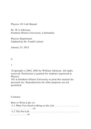
For each lab, a short summary must be written. The summary
should describe (a) the main purpose
of the lab and (b) your most important findings. The purpose of
the summary is to help you see the “big
picture”, so you shouldn’t simply repeat all of your results.
When you write the summary, make sure you
look at the objectives for the lab, and say something about each
of them. The summary should answer two
questions: “What physical principle or phenomenon did we
study?” and “What did we actually learn about
it?” The summary must be written in proper english.
-1.4 How to Draw Graphs
A sample graph is shown in Fig. 3. When you draw a graph, pay
attention to the following rules:
• All graphs need to have a title and a number. For example
“Graph 1: Radiation penetration in lead”.
-1.4. HOW TO DRAW GRAPHS ix
• When drawing a graph of “A” versus “B”, put “A” on the
vertical axis and “B” on the horizontal.
This is so that your graph shows how a measurement (on the

vertical axis) changes at intervals of the
horizonal axis (which are often intervals of time).
• Graphs should be drawn in pencil.
• Graphs must be drawn on graph paper.
• Make the graphs big. Use as much of the page as possible
BUT keep it simple. The entire page could
have been used in Fig. 3 if each square were 0.77 m instead of 1
m, but this just makes graphing
complicated, and doesn’t add anything to the final product.
• Make sure you label the axes of your graph. If the x-axis
indicates time measured in seconds, then it
should read “time (s)”.
• Make sure you draw the scale on the graph.
When you are asked to draw a smooth curve through your data,
the curve generally will not pass
through all the data points. This is justified because of there is
always a small amount of uncertainty
(known as error) in making a measurement.
If the graph is a straight line, then often we want to find the
slope of the graph. The slope of a straight
line is found by drawing a triangle like the one shown in Fig. 2,
and determining the rise (the length of the
triangle in the y-direction) and the run (the length of the
triangle in the x-direction). The slope is then
given by
slope =
rise

run
Notice that if the curve goes down, then the rise is negative and
the slope is negative. Notice also that the
units of the slope are given by the units of the y-axis over the
units of the x-axis. If the y-axis is cm, and
the x-axis is seconds, then the slope of a line on the graph is in
cm/s. Finally, remember to show your
calculations on the graph, as done in Fig. 2.
x HOW TO WRITE LABS
1 2 3 4 5 time (s)
10
15
20
5
rise = 16 m
run = 4 s
slope =
=
=
16 m
4 s

4 m/s
rise
run
Graph 2: Cart distance v. time
Figure 2: Sample graph showing how to calculate the slope.
-1.4. HOW TO DRAW GRAPHS xi
Figure 3: Sample graph for making plots.
xii HOW TO WRITE LABS
Chapter 0
Pre-Lab Questions
1
2 CHAPTER 0. PRE-LAB QUESTIONS
0.1 Pre-Lab 1: Observations of Venus and Mars
Name Section Date

You may answer these questions directly on the figures.
This section looks at the simplest orbital system: the earth and
the sun. The aim of this section is to
give you some practice connecting what we see on earth to the
earth’s orbital motion. Figure 1 shows two
views of the earth. Figure 1 (a) shows a “side-view”, with North
pointing upwards. Figure 1 (b) shows a
“top-view”, with North pointing out of the page towards you.
Question #:1 In Fig 1 (b) there are three arrows shown at point
A on the earth’s equator. The arrows
are labelled 1, 2, and 3. For a person standing at point A, which
arrow points East, which points West and
which points straight up into space?
• Figure 2 is a schematic figure (not to scale) of the earth in
orbit about the sun. As in Fig. 1 (b), the
view is from the “top”, so that North points directly out of the
page towards you. The earth is shown
at a particular instant in time.
Question #:2 The points A and B indicate two di!erent points on
the earth’s surface. At each point,
draw arrows indicating West and East (a total of four arrows),
assuming that North points out of the page
towards you. Next, using the fact that the sun rises in the East,
draw the direction of the earth’s daily
rotation.
• The time at a particular point on the earth’s surface is
determined by it’s location relative to the sun.
If the sun is directly overhead, then it is noon. On the opposite
side of the earth, where “up” points
directly away from the sun, it is midnight. At points half-way in
between midnight and noon, it is

either 6 pm or 6 am.
Question #:3 Estimate the time to the nearest hour at points A
and B.
0.1. PRE-LAB 1: OBSERVATIONS OF VENUS AND MARS 3
N
S
W
E
1
3
2
(b)(a)
A
Figure 1: Two perspectives of the earth. In (a), the four compass
directions are also shown at a particular
point on the earth’s surface in the Northern hemisphere. In (b),
the North pole points directly out of the
page towards you [ie. you are looking down from the “top” of
(a)].
A
B

Figure 2: The earth in orbit around the sun.
0.2 Pre-Lab 2: Di!usion
Name Section Date
Reading: Hobson Ch.2, section 2.1 & section 2.2
Try to understand the comment of fig.2.1 of the textbook.
Review section 2.3 of the lab on di!usion
Question #:1 Define di!usion. Hint: Look it up in Wikipedia, the
free online encyclopedia. use key
words such as molecular di!usion, Brownian motion
• Figure 3 shows a cartoon of a random walker. Initially, the
walker starts at 0. A coin is tossed and
the walker moves one position to the right if the coin lands
“heads” and one position to the left if the
coin lands “tails”. We represent the position of the walker by a
number r.
• Perform your own random walker experiment. Start at r = 0
and toss a coin 20 times. For each “tails”
subtract 1 from r, and for each “heads” add 1 to r. Record this
in a table. Note that r can be positive
or negative.
• Read the section “How to draw graphs” in the introduction to
the lab manual. Draw a graph of r vs.
N (the number of coin tosses), following the guidelines set out
in the introduction.

0-2 -1 1 2
Figure 3: The random walker. If the coin-toss is “heads” the
walker moves one step to the right; if the
coin-toss is “tails” the walker moves one step to the left. In this
figure, the walker is moving from r = 0 to
r = 1.
0.2. PRE-LAB 2: DIFFUSION 5
0 20 40 60 80 100
N (Number of coin tosses)
0
5
10
15
20
av
er
ag
e
|r|
10 Random Walkers
1000 Random Walkers

Figure 4: Average distance travelled for many random walkers.
This data is generated by having a computer
toss a coin 100 times for each random walker, and then
averaging the results.
Question #:2 Describe, in words, the relationship between r and
N for your random-walker experiment.
In other words, is there a pattern in the way r changes when you
increase N? Is there anything predictable
about the motion of your random walker?
• Figure 4 shows the average of |r| for 10 random walkers and
for 1000 random walkers. The symbol
|r| refers to the absolute value of r, which means dropping the
minus sign (if there is one) in front of
the number. Thus | ! 5| = 5, | ! 3.7| = 3.7, and |10| = 10. The
figure shows the average distance of
1000 random walkers from their starting place after 1, 2, etc.
coin tosses. This data was generated by
a computer which tossed a coin 100 times for each random
walker. The data was then averaged over
all the random walkers. The data shows that, for 1000 walkers,
the random walkers have moved an
average of 1.87 steps away from their origin after 5 coin tosses.
This means that some walkers have
moved 1 step away, some have come back where they started
from, and a few have even moved a full
5 steps away.
Question #:3 Compare the average motion of the random
walkers with your coin tossing experiment.
What do you notice about the average motion of the random
walkers as the number of walkers is increased?
Note that each individual random walker still moves completely
randomly!

Question #:4 From your graph, can you estimate what |r| will be
for your single random walker after
30 coin tosses? How much confidence do you have in your
estimate?
Question #:5 From Fig. 4 estimate the average value of |r| for
1000 random-walkers after 150 coin tosses.
How much confidence do you have in your estimate?
Question #:6 Which has more predictability, the motion of an
individual random walker or the collective
(average) motion of a large number of random walkers?
• A theory or an equation has predictive power if it can predict
the outcome of an experiment which
has not yet been performed.
0.3. PRE-LAB 3: OBSERVATIONS OF MOTION 7
0.3 Pre-Lab 3: Observations of Motion
Name Section Date
Reading: Hobson Ch.3: section 3.4 & section 3.5
Galileo found that gravity causes constant acceleration along an
incline. Assuming an object starts from
rest:
• The relationship between distance (s), acceleration (a), and

time (t) is: "s =
1
2
at2, where " refers to
the fact that the distance measurement measures the di!erence
between its position at the beginning
and end of the experiment.
• The relationship between speed, acceleration and time is: v =
at
• Keep in mind that A2 (A squared) is A multiplied by A, not A
multiplied by 2.
Question #:1
• A cart on a linear track has a uniform acceleration of
0.172m/s2. What is the velocity of the cart 4.00
s after it is released from rest?
• How far does this cart travel during these 4 s?
• From the first equation, give the expression of the
acceleleration a
In table 1 is a data set of time and distance traveled.
Question #:2
• Complete table 1
• find the average acceleration

"s(m) 0 0.25 0.50 0.75 1.00 1.25 1.50
t(s) 0.00 0.45 0.71 0.77 0.98 1.07 1.12
t2
a
Table 1: Average values of time are below the corresponding
values of distance
Question #:3 use the collected data in table 1 and:
• Plot distance versus time
• is this a uniform motion? Explain
Question #:4 use the collected data in table 1 and:
• Plot 2"s versus t2
• Give an interpretation of the slope of this graph
• Extract the average acceleration from the graph. and compare
with the previously calculated one.
0.3. PRE-LAB 3: OBSERVATIONS OF MOTION 9
Figure 5: Distance Versus Time.

Figure 6: Twice the distance versus Time squared
0.4. PRE-LAB 4: CONSERVATION OF MECHANICAL
ENERGY 11
0.4 Pre-Lab 4: Conservation of Mechanical Energy
Name Section Date
Reading: Hobson Ch.6: section 6.5 & section 6.6
• Potential energy is given by PE = mgh
• Kinetic energy is given by KE =
mv2
2
Mechanical energy
and pendulum
A
B
C
D
Figure 7: Trade in joules between potential and kinetic energy

Consider the situation in figure 7, the total mechanical energy is
6 J. There is no loss or gain of mechanical
energy, only a transformation from kinetic energy to potential
energy (and vice versa). The ball, of mass
m = 1kg is released from rest. Answer the following questions:
Question #:1 At point A:
• What is the potential energy of the ball?
• What is the height of the ball?
• What is the velocity of the ball at that point?
• What is the kinetic energy?
Question #:2 At point B, if the potentianl energy is equal to the
kinetic energy (PE = KE = 3J)
• What is the height H of the ball?
• What is the velocity of the ball at that height?
Question #:3 At point C, the potential energy is zero.
• What is the kinetic energy of the ball?
• What is the velocity of the ball at that point?
• How would you describe the velocity at this particular point?
Explain

Question #:4 At poind D, the ball is at the same height as in
point A, it reaches a maximum height
then stops before reversing direction.
• What is the potential energy?
• What is the kinetic energy of the ball?
• What happened to kinetic energy at that position?
Question #:5 While the pendulum is oscillationg between
positions, use the words increase, decrease,
or constant to describe the trend of the di!erent forms of
energies. Complete table 2
Potential Energy Kinetic Energy Mechanical Energy
From A to C
From C to D
Table 2: Trend of the di!erent forms of energy of a swinging
pendulum
Question #:6
• Using figure 7, identify the corresponding positions A , B and
C in figure 8
• Discuss the di!erent energies, and speeds of the glider on
those points based on your study of the
pendulum.
0.4. PRE-LAB 4: CONSERVATION OF MECHANICAL

ENERGY 13
glider
Incline
Figure 8: Sliding glider down an incline
0.5 Pre-Lab 5: Electricity
Name Section Date
Reading: Hobson Ch.8-section 8.1 and 8.3
Use the principles given in the Objectives part of the lab
(section 5.1) to answer the following questions:
Question #:1 Look at Fig. 9. Two charges (labelled A and B) are
placed in some object (for example, a
piece of glass or a piece of metal). Assume for the moment that
both charges are electrons. If the material
is a conductor, how will the electrostatic forces make them
move? Where will they stop?
Question #:2 How will the charges move in the conductor if
charge A is an electron and charge B is a
positive ion? Where will they stop?
charge B
charge A

charge C
Figure 9: Two charges (A and B) are placed in an object. A
third charge (C) is added later.
Question #:3 After the charges in the previous problem stop
moving, a third charge (charge C) is put
into the conductor. Do you expect it to feel a force? Give your
reasoning.
0.5. PRE-LAB 5: ELECTRICITY 15
negative
charge
conductor
Figure 10: Some extra negative charge is placed in a conductor.
How does it move?
Question #:4 How will the charges in Fig. 9 move due to the
electrostatic forces if the material in which
they are placed is an insulator?
Question #:5 Figure 10 shows a conductor that has some extra
electrons placed on it. Describe how the
excess negative charge moves? How is it distibuted when it
stops moving?
0.6 Pre-Lab 7: Atomic Spectra

Name Section Date
Reading: Hobson Ch.9.3, 9.4, 9.6, 13.6 & 13.7
The following hypothesis is a classical theory which tries to
explain why a light bulb emits light. It is
classical because it ignores the wave-like properties of atoms.
Hypothesis 1 Incandescent light comes from a tungsten filament
encased in a glass bulb.
1. Electric current passes through the tungsten filament and
heats it up.
2. Tungsten atoms vibrate randomly when heated. They move
more when they are hotter.
Question #:1 Use the fact that atoms are made of charged
protons and electrons to explain why the
random vibration produces light.
Question #:2 Consider an experiment where you produce waves
on a string by moving one end up and
down with your hand. What is the relationship between the
frequency of your hand (ie. the number of times
per second you move your hand up and down) and the frequency
of the wave on the string?
Question #:3 What do you think is the relationship between the
frequency of atomic vibration in the
tungsten filament and the frequency of emitted light? Based on
this hypothesis, what frequencies should be
present in the light emitted by the filament?

0.6. PRE-LAB 7: ATOMIC SPECTRA 17
Question #:4 If the atoms are hotter, then we can expect that
they will move faster and farther. What
do you think that this would do to the brightness of the light?
What about the color of the light?
Question #:5 What is the energy transformation which occurs
when light is produced? In other words,
where does the energy for the light come from? Give answers in
terms of both macroscopic and microscopic
energies.
0.7 Pre-Lab 8: Radioactivity
Name Section Date
Reading: Lab Manual section 7.2, Hobson Ch. 14.1-14.3
Question #:1 What are the four fundamental forces?
Question #:2 Which fundamental force holds the nucleus
together?
Question #:3 Which fundamental force is responsible for !-
decay?
Question #:4 Which fundamental force is responsible for "-
decay?
Question #:5 Write down the reaction equation for the "-decay

of 90Sr (Strontium-90).
Question #:6 Write down the reaction equation for the !-decay
of 239Pu (Plutonium-239).
Part I
Planets and Atoms
19
Chapter 1
Lab 1: Observations of Venus and Mars
Name Section Date
1.1 Objectives
1. To learn what information can be deduced about the planets
based on changes in their appearance
when they are observed over a period of several months.
2. To understand di!erences in the appearances of superior and
inferior planets.
1.2 The Earth’s Orbit
The following questions are based on Fig. 1.2. The questions
may be answered directly on the figure.

Question #:1 If Fig. 1.2 shows the position of the earth on
February 13, draw, as accurately as possible,
the position of the earth on April 13, two months later. Recall
that the earth orbits the sun in the same
direction that it rotates on its axis. The angular distance
travelled by the earth can be computed. Recall
that the earth travels 360 degrees in one year, so that in 19 days
it travels
19
365
" 360 = 18.7 # 19 degrees.
From this we can see the earth travels approximately one degree
per day. You may use this approximation
throughout this lab.
21
22 CHAPTER 1. LAB 1: OBSERVATIONS OF VENUS AND
MARS
Question #:2 Draw the new position of point A on April 13, if it
is the same time of day as shown for
February 13.
Question #:3 A star is directly overhead at midnight on
February 13. Draw an arrow showing the
direction to the star. At what time of day will the star be
directly overhead on April 13? You can figure
this out from the sketch you drew in Question 2. (see following
note as a hint)

• Note that stars are very far away, so that the arrows pointing
to the star on February 13 and April
13 will be nearly parallel. For the scale shown in Fig. 1.2
(representing the earth’s orbit by a circle a
few inches across), the nearest stars would be approximately 1
mile away.
1.3 Phases of the Moon
The “phase” of the moon refers to how it is illuminated by the
sun. The “full moon” is the phase in which
the entire side of the moon facing the earth is illuminated. A
“crescent moon” has only a small sliver
illuminated. In this section, you will examine the relationship
between the phases of the moon, and the
orbital motion of the moon.
Figure 1.3 shows the moon in orbit around the earth. The moon
is shown at three di!erent points in its
28-day orbit. The following questions may be answered on the
figure.
Question #:4 Assuming that North points out of the page, draw
the direction of rotation of the earth,
and the direction the moon travels along its orbit. The moon
orbits in the same direction the earth spins.
Question #:5 At each of the three locations shown, shade the
night side of the moon with a pencil. Note
that light comes as parallel rays from the sun, as shown in the
figure.
Question #:6 For each case, make a sketch of the moon showing
how you would see it from Earth.

1.4. THE PHASES AND ORBITAL MOTION OF VENUS 23
Question #:7 Indicate which of the three phases of the moon is
closest to “full” and which is “crescent”.
1.4 The Phases and Orbital Motion of Venus
In this section, you will make the connection between a
sequence of telescope observations of venus and
venus’s orbital motion. Venus is an inferior planet, which
means that the radius of its orbit is smaller than
that of the earth. This section is a little more complicated than
the previous sections because the motions
of both venus and the earth need to be considered.
You will be given a data sheet showing a series of telescope-
photos of venus taken over a 5 month period.
Answer the following questions regarding the data.
Question #:8 Figure 1.1 shows two possible arrangements of the
earth-sun-venus system. Which of these
corresponds most closely to the January 19 observation? Give
your reasons.
Question #:9 Why does venus change size in the photos?
Question #:10 Using the fact that North is up in the photos, how
can you tell that the observation on
Jan. 19 was made in the evening (and not just before dawn)?
Question #:11 Figure 1.4 shows the earth-sun-venus system with
the earth’s position shown on the date
of the first venus photo (Jan. 19/01). Use the data shown in the
handout to find the location of venus on

the observation dates listed below. This must be done in several
steps.
a.) First you need to determine where the earth is on the
observation dates. Make a table like the one
shown below
MARS
A. B.
E E
V V
Figure 1.1: The earth-sun-venus system.
Date Days Elapsed
since Jan. 19
Jan. 19 0
Feb. 20 32
Mar. 21
Apr. 13
May 8
The left-hand column shows the dates on which the observations
were made. The right-hand column
shows how much time has elapsed since the Jan. 19 observation.
For example, Feb. 20 is
20 + (31 ! 19) = 32 days
later than Jan. 19. This is the number of days in February (20),

added to the number of days left
in January, which is the total number of days in January (31)
minus the number which have already
happened, thus 31-19. Since we are looking for the days elapsed
since January 19th, you also have to
add the number of days already elapsed from the previous
months until January 19th, in this case zero
(though it won’t be the next month). Recall that the earth
travels one degree in one day. Complete
the table for the remaining observation dates.
1.5. MARS 25
b.) Draw, directly on fig. 1.4 and as accurately as possible, the
positions of the earth on each of the
observation dates.
c.) Next, draw as accurately as possible the positions of venus
on the observation dates. To do this, you
will need to use information contained in the handouts; the
telescope observations tell you how the size
and illumination (by the sun) of venus changes. From this, you
can determine the relative positions
of the earth and venus.
d.) Based on your results, estimate (very roughly) the length of
the venusian year.
1.5 Mars
You have also been given a series of photos of mars taken from
the Hubble Space Telescope over a period of
nearly 1 year. Mars is a superior planet, which means that the
radius of its orbit is larger than that of the

earth.
Question #:12 Compare the martian and venusian photos. Why
do we sometimes see a “crescent venus”
(only a thin sliver is illuminated) but never a “crescent mars”?
Note that the radius of mars’s orbit is bigger
than the radius of earth’s orbit.
Question #:13 Why can you often see mars at midnight, but
never venus?
1.6 Summary & Conclusions
Write a short summary of the lab which addresses the issues
raised in the Objectives. For example, you
might consider the following questions:
• How do the appearances of venus and mars change as they
move?
• Why do they change appearance?
• In what ways are they similar? Di!erent?
• What is the reason for their similarities/di!erences?
MARS
Question #:14 [Bonus Question] Are the data sheets (the photos
of venus and mars) compatible or
incompatible with a geocentric (earth-centered) model of the
solar system? Is there any feature of the data
which can be used to rule a geocentric model out?

1.6. SUMMARY & CONCLUSIONS 27
A
B
Figure 1.2: The earth in orbit around the sun.
MARS
Moon
Earth Light from Sun
Figure 1.3: The moon in orbit around the earth.
Earth: 01/19/01
Figure 1.4: The earth-sun-venus system.
MARS
Earth: 08/23/94
Figure 1.5: The earth-sun-mars system.

Chapter 2
Lab 2: Di!usion
Name Section Date
2.1 Objectives
This lab studies several important concepts:
1. The concept of predictive power.
2. The microscopic model of di!usion.
3. The di!erence between the microscopic and macroscopic
motion of ink molecules in water.
2.2 Di!usion of Ink in Water
• Fill the bottom of the petrie dish with a thin layer of water.
Read the instructions below thoroughly
before beginning your experiment.
• Set the petrie dish on top of the ruler so that the centimeter
scale of the ruler is clearly visible and
passes through the center of the dish, as shown in Figure 2.1.
• Make a table like the one below:
Time (s) Position of Position of d (cm)
left edge (cm) right edge (cm)
31

32 CHAPTER 2. LAB 2: DIFFUSION
Position of
Left Edge
Ink Spot
Position of
Right Edge
Petrie Dish
Figure 2.1: Experimental Setup for Di!usion Lab.
• In the first three columns you will record the position of the
left and right edges of the ink drop at
di!erent times as it expands. List the times before you start
based on the instructions below. In the
fourth column you will record the diameter d of the ink-drop.
• Carefully place a small ink drop near the middle of the petrie
dish, over the edge of the ruler (as shown
in Figure 2.1) and start timing. You need to centre the ink drop
on the edge of the ruler so that you
measure its diameter.
– If you don’t get a nice compact ink drop, you should start
again. It may take several tries.
– This experiment works best if the water is at room
temperature. If the water is too cold, you
will get convection currents.

• Use the clock on the wall or your cellphone to time the
experiment. Make measurements of the
positions of the left and right edges of the ink-drop at 15 second
intervals for the first two minutes.
After two minutes, make observations every 30 seconds.
Continue until at least 180 seconds (3 minutes)
have passed.
• Make a graph of the ink-drop diameter d vs. the elapsed time.
Instructions on how to draw graphs
are given in the introduction. Draw a smooth curve through the
data points.
Question #:1 Describe in words the relationship between d and
t. Is it predictable?
2.3. MICROSCOPIC MODEL 33
Figure 2.2: The path of an ink molecule (the large gray
molecule) through water (the small black molecule).
Question #:2 The ink-spot expands more slowly at large times.
Does this mean that the individual
molecules are slowing down?
2.3 Microscopic Model
Consider a simple model for di!usion, illustrated in Fig. 2.2.
This is the microscopic di!usion model.
1. The Petrie dish contains two types of molecules—ink
molecules and water molecules. The molecules
move in random directions.

2. Ink molecules move in a straight line until they bump into
another molecule.
3. During a collision, a molecule is scattered in a random
direction. (In fact, the direction isn’t really
random. If we knew the details of exactly how each collision
occured then the direction of the molecules
after each collision could be predicted exactly.)
4. The molecule continues moving in a straight line until it
bumps into another molecule.
5. Because of this random scattering the ink molecules move in
a random walk. This means that the
motion of an individual molecule is unpredictable.
6. Even though the motion of each individual molecule is
random, the collective motion (ie. the average
motion of many ink molecules) is predictable. This collective
motion is called di!usion.
7. The rate at which molecules di!use is measured by the
“Di!usion constant” D. A large value of D
means that molecules spread out quickly.
8. The di!usion constant D is determined by the kind of
molecules di!using, by the medium through
which they di!use, and by the temperature.
Question #:3 The speed of a molecule is determined by its
temperature (hot molecules move faster).

How will temperature a!ect the di!usion constant D? Why?
Question #:4 Since molecules are father apart in gases, they
travel farther between collisions. Will D
be larger or smaller in gases than in liquids? Why?
• If di!using molecules can be thought of as random-walkers,
then it should be possible to make a
connection between the microscopic di!usion model and the
coin tossing experiment.
• The following questions try to show that the coin-tossing
experiment is a useful “toy-model” for
di!usion. That means it is a simplified model which contains the
basic ingredients to explain di!usion.
Question #:5 Assume that the coin-tossing experiment can
explain di!usion. What element of the mi-
croscopic di!usion model does the random-walker itself
represent?
Question #:6 What microscopic property of the ink molecules
does the variable r from the coin tossing
experiment represent?
Question #:7 What element of the microscopic di!usion model
does the variable N from the coin tossing
experiment represent?
Question #:8 What does each coin toss represent?
Question #:9 What macroscopic property of the ink spot does

the average r represent?
What have we done here? This lab has many pieces to it so it
can be a bit confusing. We studied a “random
walker” model of di!using molecules. In order to check whether
this model works, we made a prediction
that we could test. In this case, the prediction had to do with
how the size of the ink spot changes with
time.
Question #:10 Compare your graph of d vs. t with the data for
the average |r| vs. N shown in Fig. 4.
Are these two graphs consistent with each other? In other
words, does your graph of d vs. t support or
contradict the random walker model of di!usion?
Question #:11 Does this experiment prove that molecules exist?
Does it support the theory that
molecules exist? Justify your answer.
• Now write a brief discussion of the lab based on the
objectives. You can turn each objective into a
question by starting it with “What is. . . ”
Question #:12 Bonus Activity: If you perform the ink spot
experiment with cold water (the colder
the better), then after a minute or two of observing, you should
see convection cells form. Describe what
you see, especially as it is di!erent from when you did the
experiment with warmer water. Draw pictures if

it will help.
Part II
Newton’s Universe
41
Chapter 3
Lab 3: Observations of Motion
Name Section Date

3.1 Objectives
• To study the motion of a glider on incline
• To understand the concept of acceleration
3.2 Motion on an Inclined Air Track
In this section, you will study the motion of a body accelerating
under gravity. These experiments are
very similar to ones performed by Galileo in the 17th century.
He studied the motion of rolling balls on an
inclined plane, and deduced, among other things, that falling
bodies accelerate uniformly.
This lab examines acceleration more closely. You will look at
the motion of a glider on an inclined air
track. Your TA will demonstrate the use of the air track and
photogate with the accessory photogate.
• First, level the air track. You can do this by adjusting the
threaded legs on the track. When the air
is on, the glider should remain stationary when you release it.
• Now, elevate the air track by turning the adjustable legs
through 5 complete turns. (The end marked
“140 cm” should be higher than the end marked “0 cm”).
• Make a table like the one below
43
44 CHAPTER 3. LAB 3: OBSERVATIONS OF MOTION

glider
s
s1
2
adjustable legs
Figure 3.1: Schematic diagram of the air track.
Table 1: Motion on an air track
elevated by 5 turns
Position s1 Position s2 Distance "s Time t1 Time t2 Time t3
average time t
(cm) (cm) (cm) (s) (s) (s) (s)
10 20
10 30
10 40
10 60
10 80
10 130
3.2. MOTION ON AN INCLINED AIR TRACK 45
Here s1 is the initial position of the glider measured at the
leading edge of the glider, and t1, t2 and t3
are the times required for the glider to travel to the end of the

inclined plane on three di!erent trials.
• Place leading edge of the the flag on top of the glider just
before the 10 cm mark (at s1) on the inclined
plane, along with the accessory photogate. Make sure the switch
on the photogate is set to pulse mode
and the other switch is set to the on position. Release the glider
just before the position that it will
trip the photogate, without giving it any sort of a push forward
or backward. The photogate should
time how long it takes to travel to the other photogate,
positioned at s2 on the air track. Record your
answer in the table in the column labelled t1. Repeat the process
twice more and record the answers
under columns t2 and t3. Record the average of t1, t2, and t3 on
the chart.
• Calculate "s = s1 ! s2, which is the total distance travelled by
the glider. Record the value in the
column marked ’Distance "s’
Question #:1 List at least 2 important sources of error. In other
words, give two reasons why t1, t2 and
t3 di!er from each other.
• Using the graph paper provided, carefully make a graph of "s
versus t, using the average t. Draw a
smooth curve through the data points (remember, you don’t
need to hit each one, just give a good
idea of the trend with your line). When you draw the curve,
remember that when "s = 0 cm, t = 0
s. A neat graph will make some of the following questions
easier.
Question #:2 Based on your graph, does the glider speed up,
slow down, or travel at a constant speed

as it moves along the track? Hint: Estimate how far the glider
moves in the first second, and in the last
second.
Question #:3 What is the average speed of the glider during the
last run (starting at s1 = 130 cm)?
Don’t forget to show your calculation. Recall that average speed
is equal to the distance divided by the
total time.
• You have seen in class that the instantaneous speed can be
found from the slope of the "s versus.
t graph. Pick three (approximately) evenly-spaced values of t on
your graph which cover the whole
range of times measured in the experiment (that is, pick points
at the beginning, middle and end).
• At those three points from the graph, draw a tangent line to
the smooth curve you drew through your
data. A tangent line is a line which grazes against a curved line,
touching it but coming out on the
same side of the curve on both directions before any
intersection.
• Find the slope of the tangent line at each selected time.
Instructions for finding slope are found in the
Introduction to the lab manual. You will use points on the
tangent line. The points you use to find
the slope which are not on your smooth curve will not be used
after this. This slope has units of cm/s
and is the speed of the glider at that instant in time.

• Record your results for each tangent line in the table below:
Table 2: Speed of the glider down the incline
Time t in seconds Distance "s in cm Speed v in cm/s
Question #:4 Compare the instanteneous speeds you calculated
with the average speed of the glider you
calculated earlier. (for s1 = 130cm)
3.3 The Concept of Acceleration
• We can define acceleration to mean that the speed of the
glider increases as it moves down the track.
The speed of the glider changes with respect to position and
time. If you think about it for a minute,
you will find that this is ambiguous. Galileo had to to struggle
with the idea of acceleration.
Definition: The average accelaration over some time interval tf
! ti is given by
a =
vf ! vi
tf ! ti
where vf ! vi is the change in speed over the interval. Here, ti
and tf are the beginning and ending
points of the time interval, and vf and vi are the speed of the
glider at tf and ti.
– Using the data you recorded in Table 2, make a graph showing
the speed of the air glider versus
the total time t the glider has moved.
– Draw a smooth curve through your data.

Question #:5 Describe the relationship between the speed of the
glider and the time it travels. Is
there a predictable pattern? Can you predict the speed of the
glider after 30 s?
– From the definition, we can define an instantaneous
acceleration by making the distance interval
tf ! ti very small. This is equivalent to finding the tangent to the
curve.
– Plot the three points from table 2 in a graph of speed vs time.
Does the graph look linear (close
to a straight line)? Find the slope of a line between the first and
last points.
Question #:6 What are the units of acceleration (based on the
definition earlier)?
Question #:7 Does the acceleration change as the glider moves
down the air track? Explain.
Question #:8 From a series of careful experiments, Galileo
determined that the acceleration of a
body down an inclined plane is uniform (constant) provided he
used Definition 2 for acceleration. Do
your results support this? Do you find any significant deviations
from Galileo’s theory? (“Significant”
means you can’t simply blame them on human error in the
timing.)
Question #:9 If you change the elevation (ie. the steepness) of
the air track, how do you think that

this will change the relationship between v and t. Will the
shapes of the curves change? If so, how?
Summarize your main findings in this lab. What did you set out
to investigate and what did you find?
Remember to address the objectives for the lab.
Figure 3.2: Graph of distance traveled versus the average time:
"s Versus tav
Figure 3.3: Speed of the glider Versus the time it travels down
the incline.v Versus t
Chapter 4
Lab4:Conservation of Mechanical Energy
Name Section Date
4.1 Objectives

In this laboratory experiment, we are going to illustrate the
conservation of mechanical energy:
– Quantitatively: through measurement and data analysis
– Qualitatively: through graphical analysis
4.2 Definitions
– Gravitational Potential Energy is an energy by virtue of
position: PE = mgh
– Kinetic Energy is an energy of motion: KE =
mv2
2
– Mechanical Energy: ME = KE + PE $ ME =
mv2
2
+ mgh
4.3 Theory
The Total Mechanical Energy of an object remains constant in
the absence of nonconservative forces
like friction. The conservation of energy is a fundamental tenet
of science and has extremely broad
applications in all technical fields. The two types of energy that
will be under consideration in this
laboratory experiment are the gravitational potential energy PE
and the kinetic energy KE. The object
in this case will be a glider on an air track system. There are
two forces at work in this experiment -

gravity and friction.
51
52 CHAPTER 4. LAB 4: CONSERVATION OF MECHANICAL
ENERGY
The frictional forces have been minimized by the use of the air
track system and will therefore be
neglected in our analysis. Gravity exerts a force on the glider
and will contribute a gravitational
potential energy (PE) to the Total Mechanical Energy. The
normal force of the track pushing back
on the glider is perpendicular to the direction of the glider
motion and so will produce no work and
will not a!ect ME.
Therefore, in this experiment the Total Mechanical Energy
consists only of the Kinetic Energy (KE)
and the Gravitational Potential Energy (PE). Since there are no
non-conservative forces acting on the
glider its Total Mechanical Energy is conserved.
4.4 General Procedure
– As the glider accelerates down the sloped air track you will
make measurements of the glider’s
PE and KE for six di!erent locations along the air-track.
– These six positions are located at 20 cm, 40 cm, 60 cm, 80
cm, 100cm and 120cm marks along
the length of the track.
– The glider’s PE can be calculated if we know its vertical
height from the reference level of zero

gravitational potential energy. We will choose the zero
reference level to be the height of the
sixth (bottom) y6 which corresponds to 120cm-mark on the air-
track.
– We will first measure the heights of each of the measurement
positions relative to the surface of
the table and record these in the first column of your Data Table
4.1.
– Then subtract o! the height that you measured for the sixth
(bottom) position y6 from all six of
the measured height values.
– Record these results in the second column of your Data Table
4.2.
– The velocity needed for calculating the glider’s KE will be
measured at five locations along the
air track using the photogate. The TA will demonstrate how to
use the photogate.
– The velocity of the glider, v, at each measurement location
will be determined by the photogate
which will time the passage of a narrow flag (a piece of paper
or notecard carefully folded multiple
times), mounted in the front of the glider as it passes through
the photogate.
– Since the glider is at rest at the first location y1, the KE at
that position is zero.
– After you place the photogate at one of the measurement
locations and let the glider accelerate
down the air track the photogate will provide the timing
information that together with the flag

length will enable you to calculate the glider’s average velocity
at the measurement location:
v =
L
"t
– After each velocity is calculated, record it in your Data Table
4.1.
– Once all the velocity-positions data have been collected, you
will calculate the values of the three
quantities, PE, KE, and ME = KE + PE and record them in your
Data table 4.2.
4.5. DETAILED PROCEDURE 53
0
y6
y5
y4
y3
y2
y1
100
80
40

20
60
120
Figure 4.1: glider-air track system: heights yi & positions along
the incline
– Then you will plot each of these three variables versus
position of the glider along the air track.
– These plots will allow you to test the validity of the claim that
Mechanical Energy, as applied to
our simple glider and air-track system, is conserved.
4.5 Detailed Procedure
– For better results, all of your observations should be recorded
to 3 significant figures. You should
carry 3 significant figures (three digits) in all of your
calculations as well.
– Measure the mass of your glider using the available scale and
record here M = g, kg
– Measure the length of the flag of the glider using the provided
Caliper and record the length here
L = mm, m.
– (Optional) Place a jack or a block of wood under the single
leg of the air track. Set up the
air-track with an inclination roughly similar to that shown in
figure 4.1
– The initial vertical height measurements are denoted by the

variable yi. The measurements should
be made using the calipers from the bottom of the air track to
the table top at positions located
at 20cm, 40cm, 60cm, 80cm, 100cm, and 120cm along the air
track.
– The launching point should be the same ( position 20 cm on
the airtrack) for all trials.
– We will designate the height y6 as the zero reference level of
the gravitational PE.
– The di!erence in heights relative to this zero level will be
designated by the variable h defined as
hi = yi ! y6.
ENERGY
– Measure y1 through y6, as shown in figure 4.1, to three
significant figures. Calculate the hi values
and record them in your Data Tables 4.1 and 4.2
– Place the photogate at the first data collection point, s =
40cm. Switch the photogate to GATE
mode. Make sure to RESET gate before each time you take data.
– The photogate should be rotated slightly about its mounting
axis so that its body is perpendicular
to the plane of the air track. The flag should not strike anything
as the glider travels down the
air track. The flag should be flush with the forward edge of the
cart. After taking data at this
point this alignment procedure will be repeated at each of the

other positions
– Turn on the air supply to the air track. The glider will float on
a cushion of air.
– Let the glider accelerate from its rest position at poistion
20cm mark.
– Record the velocity measured, when the glider passes through
the photogate, in the Data Table
4.1. Repeat this velocity measurement two more times for a
total of three velocity measurements
at each photogate position.
– Repeat these velocity measurements with the photogate
positioned at the remaining locations,
and record the values in the corresponding Data Tables 4.1.
– Calculate the average velocity for each measurement location
and record the results in both
tables.
Complete table 4.1 remember that hi = yi ! y6.
Complete table 4.2. Assume g = 9.8m/s2
4.6 Analysis
After completely filling in the two data tables, you are ready to
answer questions and make your
graphs.
Question #:1
– What is the gravitational potential energy of the glider at the
very top (y1 position)?

Show your calculation in the space below
– Is it maximum or minimum?
– How is it compare to the total mechanical energy?
4.6. ANALYSIS 55
Question #:2
– At the height y3, what fraction of the total mechanical energy
is gravitational potential energy?
Show your work.
– Could you have qualitatively predicted such an outcome?
Explain.
– What will happen to the potential energy as the glider slides
downward?
Question #:3
– What is the kinetic energy of the glider at the very bottom (y6
position)?
Show your calculation in the space below
– Is it maximum or minimum?
– How is it compare to the total mechanical energy?
– what is the potential energy at this location?
– What happened to the potential energy?

ENERGY
Question #:4
– In this lab we neglected friction. If friction was present what
would it do to the values of the
velocities?
– How would this a!ect the kinetic energy values?
– What would this do to the value of the Total Mechanical
Energy (ME)?
– Make a general statment about the e!ect of friction on a given
system. ( will it add or remove
energy)
4.7 Graphical analysis
In this section, we will discuss the conservation of mechanical
energy graphically. The vertical scale
will be used to represent energy in joules and the horizontal
scale will be used to represent the positions
in centimeters. Use the data collected in table 4.2. Plot
everything on the same graph.
1. Plot of potential energy versus position ( PE Vs s):
– Draw a smooth curve or line through the data
– Describe the trend of the curve ( increasing, decreasing or
constant)

2. Plot of kinetic energy Versus position ( KE Vs s):
– Draw a smooth curve or line through the data.
4.8. SUMMARY & CONCLUSION 57
– Describe the trend of the curve (increasing, decreasing or
constant)
3. Plot of mechanical energy versus position( ME Vs s):
– Draw a smooth curve or a line through the data.
– Describe the trend of the curve (increasing, decreasing or
constant)
– How can you tell from the graph that PE + KE = Constant
4.8 Summary & Conclusion
Question #:5
– Within reasonable limits of this experiment, were you able to
test the validy of the following
claim: ”in the absence of non-conservative forces(friction), the
mechanical energy for the glider
on the air track is conserved”. Explain.
– ”Energy is generally conserved. Mechanical energy is
conserved when frictional forces are mini-
mized.” True or False?

ENERGY
Figure 4.2: Kinetic, Potential & Mechanical Energy Versus
Position
4.8. SUMMARY & CONCLUSION 59
Position: si Height: hi Repeated measurement of time: ti
average velocities vi
t1 = vav1 =
flag length
tav
20 cm h1 =
t2 =
t3 =
tav =
t1 + t2 + t3
3
= vav1 =
t1 =
40 cm h2 =
t2 =
t3 =

tav =
t1 + t2 + t3
3
= vav2 =
t1 =
60 cm h3 =
t2 =
t3 =
tav =
t1 + t2 + t3
3
= vav3 =
t1 =
80 cm h4 =
t2 =
t3 =
tav =
t1 + t2 + t3
3
= vav4 =
t1 =
100 cm h5 =
t2 =

t3 =
tav =
t1 + t2 + t3
3
= vav5 =
t1 =
120 cm h6 =
t2 =
t3 =
tav =
t1 + t2 + t3
3
= vav6 =
Table 4.1: Repeated measurement at each position leading to
vavg needed for evaluating KE
ENERGY
Position s yi vertical hi = yi ! y6 height hi PE = mgh vavg KE =
mv2
2
ME = PE + KE

(cm) (mm) (mm) (m) (J) (m/s) (J) (J)
20
40
60
80
100
120
Table 4.2: Data leading to KE, PE and their sum
Part III
The World of Electricity
61
Chapter 5
Lab 5: Electricity
Name Section Date
5.1 Objectives

To study some consequences of three fundamental principles of
electricity:
1. Like charges repel, and unlike charges attract.
2. Electrons, which are negatively charged, move freely in a
conductor, but cannot move through
an insulator. Positive charges cannot move in solids, even if
they are conductors.
3. A neutral material has as much positive charge as negative
charge.
You should be able to explain all the observations you make in
this lab with these ideas.
5.2 Electrostatics
– Figure 5.1 shows the electroscope. The essential feature is
that two gold-foil leaves hang from a
metal rod connected to a conducting ball. To begin with, make
sure the leaves hang freely.
– Rub a piece of acetate (the clear cylindrical plastic rod) with a
dry and clean piece of paper and
bring the acetate close to the silver conducting ball on the top
of the electroscope. Then, touch
the conducting ball on top of the electroscope with the acetate.
Next, touch the ball with you
hand. Next, repeat the process with the aluminum bar.
– Note: Sometimes the gold foil leaves will stick to themselves
or to the glass plates on the front of
the electroscope. This is undesirable, and you should try to
avoid it when you do the experiments.

63
64 CHAPTER 5. LAB 5: ELECTRICITY
plastic cork
metal rod
metal foil leaves
conducting ball
Figure 5.1: The electroscope
5.2. ELECTROSTATICS 65
Question #:1 Describe carefully what you observe as you
perform the above experiments.
Question #:2 The acetate is positively charged after being
rubbed with the paper. Use this fact to
explain your observations. Specifically, explain
1. how electrons move in the electroscope as you bring the
acetate close (but not touching) to the
electroscope. Make a sketch of the electroscope and acetate
strip showing regions of positive and
negative charge.
2. how electrons move when you touch the acetate to the
conducting ball. Again, make a sketch of
the electroscope and acetate strip showing how charge flows,

and what the final charge distribu-
tion looks like after the acetate strip has been taken away.
3. why the gold-foil leaves move in each case.
4. what happens to the charge on the electroscope when you
touch it with your hand.
Question #:3 The gold foil is connected to the ball by a metal
rod, and this experiment shows that
charge can be transferred through the rod to the gold foil. Why
does the experiment not work when
you touch the electroscope case with the acetate instead? (Try
it).
– Ground the electroscope by touching the silver ball with your
hand. The gold foil should return
to its neutral “resting” position.
– Now, rub the vinyl strip (the grey rod) with the paper and
touch the strip to the silver ball on
the electroscope.
– Then, rub the acetate strip with the paper and bring it close to
the ball on the electroscope.
– Finally, touch the acetate to the silver ball.
Question #:4 Describe carefully what you observe in the above
steps.
Question #:5 What do your observations tell you about the

charge on the vinyl strip? Give clear
reasons. Make sketches showing (a) how charge moves when
you bring the vinyl strip close to the
electroscope and (b) how charge moves when you touch the
electroscope with the vinyl strip.
– Ground the electroscope by touching the silver ball with your
hand.
– Charge the electroscope with either the acetate or vinyl strip.
– Several pith-balls, which can be suspended by a nylon thread,
are provided. Ground a pith ball
by touching it with your hand. Then hold the pith-ball by the
nylon thread, so it can swing freely
and bring it slowly closer to the electroscope (without swinging
it). Look carefully for the e!ects.
Question #:6 Describe carefully what you observe happening
before, during, and after contact
occurs between the pith-ball and the electroscope. Things
happen quickly, and can be hard to see, so
you may want to repeat this experiment several times. Also,
note whether the gold-foil moves.
5.3. THE CONCEPT OF “GROUND” 67
Question #:7 Explain your observations in terms of the motion
of electrons. Note that the pith-ball
is a conductor, and that your answer to question 3 is important
here. Divide your explanation into
three categories:
1. Before the pith-ball makes contact with the electroscope.

2. During contact.
3. After the pith-ball makes contact with the electroscope.
5.3 The Concept of “Ground”
The concept of “ground” is extremely important in electricity. It
refers to the fact that, given the
chance, excess electrical charge will almost always flow into
the earth. The next few questions elaborate
on this point.
Think of the earth as a giant conducting sphere (yes, dirt
conducts electricity, though not particularly
well). Use the principles outlined in the Objectives and think
about your answer to the last prelab
question to answer the following questions:
Question #:8 Why does touching the electroscope with your
hand discharge it completely, but
touching it with a pith-ball only discharge it a little bit?
Question #:9 Given the choice, why would excess charge on the
electroscope prefer to flow into
the earth, rather than into (for example) your body?
Question #:10 All modern electrical appliances are “grounded”.
This means that the metal exte-
rior of your toaster is connected to the earth by a wire. Why?
(Hint: This is a safety feature. Think
about what would happen if a wire was broken and touched the

side of the toaster.)
5.4 Conductors and Insulators:
– Most materials fall into one of two categories: either they are
electrical conductors or electrical
insulators. In fact, almost nothing is a perfect conductor or
insulator, and most materials fall in
between.
– We can describe how good a conductor a material is using the
concept of electrical resistance.
If the resistance is low, the material is a good conductor. If the
resistance is high, the material
is a poor conductor. A perfect conductor has no resistance and a
perfect insulator has infinite
resistance.
– Fill out the table below using the instructions described
afterwards:
Material Resistance
aluminum rod
plastic rod
glass rod
wooden block
human hand
copper wire
air
5.5. SIMPLE CIRCUITS: 69

+-
Power SupplyLight bulb
Figure 5.2: A simple electrical circuit.
– Charge the electroscope with either the vinyl or acetate strip.
Then discharge the electroscope
by touching the conducting ball with the aluminum bar. Notice
(roughly) how long it takes for
the electroscope to discharge, and use this to determine the
resistance of the bar.
– In the second column, indicate whether the electrical
resistance is low, medium, or high.
– Repeat the process for each material provided, as well as any
others you want to include.
Question #:11 When electricity was first introduced into homes,
many people were nervous about
the fact that electrical sockets didn’t have plugs. They were
worried that if nothing was plugged into
the sockets, electricity would leak out of the holes into the
room. Why doesn’t electricity leak out of
electrical sockets?
5.5 Simple Circuits:
So far, you have established that electrons can flow through
conductors, and that they will do so (a)
to move away from areas of excess negative charge (b) to move
towards areas of excess positive charge.
This flow is called an electrical current. Electrical currents are
useful to us because we can make the

electrons do work while they move.
You can think of a power supply as a device which builds up
excess positive and negative charges on its
two terminals. If some conducting path is available, electrons
will flow between the terminals because
of the forces between the charges. In the next experiments, the
electrons will do work illuminating a
lightbulb as they flow.
The important di!erence between a power supply (like a battery)
and the electroscope is that the
power supply replenishes the charge on its terminals whenever
it is depleted.
– Construct the simple circuit shown in Fig. 5.2. The “-” sign on
the power supply indicates that
there is a surplus of negative charge at that terminal.
Power SupplyLight bulb
+-
Aluminum Bar
Figure 5.3: A more complicated electrical circuit.
– When the power supply is turned on, the lightbulb is
illuminated, indicating that electrons are
flowing through the circuit.
Question #:12 Draw a sketch like Fig. 5.2 and show the

direction electrons flow through the wire.
Why do they flow in this direction? (Hint: Think about the
forces on the electrons.)
Question #:13 Describe what happens if you insert a piece of
aluminum into the circuit? (See Fig.
5.3) What about a piece of wood? What about some of the other
materials you looked at earlier?
Summarize briefly what this lab demonstrated. Think about the
following questions: What makes
electrical charges move? What factors a!ect how much charge
moves? Why is the concept of resistance
useful for describing this?
Question #:14 Di!erent materials have di!erent electrical
properties. For example, glass is an
insulator, and aluminum is a conductor. Is it (a) because they
contain di!erent numbers of electrons
or (b) because the electrons move more freely in some materials
than others? Is there any evidence
from this lab you can use to support your answer?
Part IV

Within the Atom
73
Chapter 6
Lab 6: Atomic Spectra
Name Section Date
Caution! The fluorescent gas tubes used in this lab are delicate,
and become very hot
during use. Be careful when you handle them. The fluorescent
gas tubes in this lab
may contain mercury. Mercury is poisonous. If you break a gas
tube, notify your TA
immediately.
6.1 Objectives
1. To compare the spectra of a tungsten filament, a fluorescent
light tube, and hydrogen tube with
each other.
2. To study two di!erent theories of light emission.
6.2 The spectroscope and the visible spectrum
– The eyepiece of the spectroscope contains a di!raction grating
which breaks light up into its
constituent colors. Use the spectroscope to look at an

incandescent light bulb. The colors in the
light emitted by the bulb will appear to be superimposed on a
scale, as shown in Fig. 6.1(b).
The scale tells you the wavelength of the light in hundreds of
nanometers (nm). Recall that 109
nm is 1 m. Also recall that for multiplying scientific notation,
the exponents belonging to the
power of ten add, and for dividing the exponents subtract, so
that
105
10!3
= 108 since 5!(!3) = 8.
If you have a scientific calculator, you might have a button with
an E on it, which denotes
scientific notation. With this notation 4E5 = 4 " 105. Do not
confuse this with the button which
says e, which stands for a number approximately 2.72.
75
76 CHAPTER 6. LAB 6: ATOMIC SPECTRA
spectroscope scale
diffraction
grating
eyepiece
slit

4 5 6 7
400 nm 700 nm
Figure 6.1: Spectroscope and spectroscope scale (for the old
spectroscopes no longer used in the lab).
Question #:1 Make another table like the one shown below. This
one does not have enough room.
Table 1: Spectrum of the Incandescent Bulb
Color Approx. Range of Wavelengths
(nm)
Use this table to record what you see when you look at the
spectrum of the incandescent bulb. In
the table, indicate the colors you see, (use 6-7 names for basic
colors that you see), and the range of
wavelengths you see them in.
6.2. THE SPECTROSCOPE AND THE VISIBLE SPECTRUM
77
Question #:2 What color has the longest wavelength? What
color has the shortest wavelength?
What colors are the brightest and dimmest? Wavelength is
measured by the placement of the color
on the scale, not the length the color seems to exist for.
Question #:3 Why do you think the spectrum cuts o! beyond
certain wavelengths? Does it mean
that the lightbulb only produces the colors you see?

Question #:4 Light with wavelengths shorter than about 400 nm
is called “ultraviolet”, and light
with wavelengths longer than about 650 nm is called “infrared”.
Why is this?
Question #:5 The relationship between wavelength and
frequency is
f =
c
#
or # =
c
f
where c is the speed of light, # (the Greek letter “lambda”) is
the wavelength measured in metres and
f is the frequency in Hertz (Hz). The speed of light is c = 3 "
108 m/s. What is a typical frequency
of red light? What is a typical frequency of violet light? Show
your calculation.
Question #:6 What aspects of spectrum of the light bulb does
Hypothesis 1 in the pre-lab describe
correctly? Are there any predictions it makes which are
incorrect?
6.3 Spectra of Gases

– Use the spectroscope to study the spectrum of one of the
overhead fluorescent lights.
– Now use the spectroscope to study the spectrum of hydrogen.
Question #:7 Describe the two spectra carefully. How do they
compare with each other and with
the spectrum of the incandescent light bulb?
Question #:8 Can your observations be explained in terms of
random motion of electrons in the
gas tubes? Why or why not? (Think carefully about this
question when you write your conclusions
at the end of the lab).
6.4. MEASURING SPECTRA 79
6.4 Measuring Spectra
6.4.1 Calibrating the Spectroscope
– To see how accurate the scale in the spectroscope is, it can be
compared to a known source.
– Look at the hydrogen tube with the spectroscope and measure
the wavelengths of the lines.
Notice that you can adjust their width using the screw at the end
of the spectroscope (don’t force
the screw). Wider lines are easier to see, but more exact
measurements come from thinner ones.
– Complete the table below:

Calibration Data
Measured # Actual # Actual!Measured
(from chart) (correction)
(nm) (nm) (nm)
The correction is the di!erence between the actual # and the
measured #.
– Be sure to note whether the measurements are too low or too
high.
– Be sure to not whether the correction is biggest at red
wavelengths or at violet wavelengths.
6.4.2 Measuring Unknown Gases
– There are several unknown tubes provided.
Question #:9 Compare their spectra with the wall chart. What
are the unknown gases? Match
each one up to a substance. Distinguish the gasses either by
numbering shown on the boxes, or by
what color they seem to glow (without a spectroscope).
6.5 Bohr’s atomic model and Plack’s constant
Neils Bohr proposed a quantum theory of light emission from
atoms. You will learn more about this
theory in class. For now, all you need to know is:

Hypothesis 2 According to Bohr’s theory, the gas tube is
produces light at only certain specific fre-
quencies. The allowed frequencies are:
f = Z " (3.29 " 1015)
!
1
n2
!
1
m2
"
where Z is the number of protons in the nucleus of the gas atom
(Z = 1 for hydrogen, Z = 2 for
helium, and so on). The numbers n and m can be 1, 2, 3 . . . and
we only consider m > n.
Question #:10 Complete the table below using Bohr’s formula
for the predicted spectrum of hy-
drogen. Note that you are only calculating a small fraction of
the possible frequencies.
m n f # #
(Hz) (m) (nm)
3 1
3 2

4 2
5 2
Question #:11 Which of the wavelengths you just calculated are
visible?
Question #:12 How well do your calculated lines compare with
the spectrum you measured.
Go back and look at the objectives for this lab. Write a brief
summary of your findings, making
sure you address the issues raised in the objectives. Remember:
you studied two hypotheses for light
emission. How well did they work? How are they di!erent?
What things do they get right? What
things do they get wrong? Could either of the theories be used
to explain both the tungsten filament
and the hydrogen gas tube?
Question #:13 [Bonus Question] Now consider helium (Z = 2).
Calculate the wavelength of
light produced in the transition of an electron from m = 4 to n =
3. Show your calculations clearly.
How does the calculated wavelength compare with the spectrum
on the wall chart.

Chapter 7
Lab 7: Radioactivity
Name Section Date
Caution: Liquid nitrogen is extremely cold and can cause severe
damage if it makes
prolonged contact with skin. Spills are especially dangerous if
the nitrogen soaks into
clothing.
7.1 Objective
1. To study background radiation.
2. To determine the kinds of radiation emmitted from a lead-210
sample.
3. To determine the levels of the various kinds of radiation
emitted by the lead-210 sample.
7.2 Radiation
7.2.1 Kinds of radiation
– Alpha (!) particles: Very large nuclei may spontaneously emit
an alpha particle. For example,
Americium, which is near the bottom of the periodic table,
decays this way. The !-particle
is a helium (He) nucleus consisting of two protons and two
neutrons. It is therefore positively
charged. !-particles, which are relatively heavy, will produce

straight dense trails in a cloud
chamber. !-particles have a range of less than 8 cm in air, and
can be stopped by a piece of
paper.
– Beta (") particles: If a nucleus has too many neutrons the most
likely form of radioactive decay
will be the emission of an electron from the nucleus. These
high-energy electrons are known as
beta particles. The "-particle is formed by the instant
transformation of a neutron into a proton
83
84 CHAPTER 7. LAB 7: RADIOACTIVITY
plus an energetic electron which then escapes from the nucleus.
"-particles are light and leave
wispy, irregular trails. "-particles have a typical range of 10–
10000 cm in air, and 0.01-10 cm in
water, depending on how fast they are travelling. "-particles are
negatively charged.
– Gamma ($) rays: After each of the previous types of
radioactive decay the new nucleus will have
an excess of energy and this is usually released by the emission
of one or more gamma-rays .
$-rays are electromagnetic radiation similar to radio waves,
visible light, and X-rays, except that
they have a much higher frequency (or shorter wavelength). $-
rays will penetrate to great depths
in materials, and no amount of absorber will completely stop all
of the gamma radiation . What
is usually done in practice is to use su#cient thickness of an

absorber to reduce the radiation
level to an acceptable value. $-rays have no charge, and are
di#cult to see in a cloud chamber.
– Cosmic rays: When there is no radiation source, cosmic rays
may enter the chamber, producing
thin misty trails. Cosmic rays are extremely energetic particles,
primarily protons, which originate
in the sun, other stars and some of the violent events which
occur in space. The cosmic ray
particles interact with the upper atmosphere of the earth and
produce showers of lower energy
particles. Many of these lower energy particles are absorbed by
the earths’ atmosphere as they
travel down to the surface. At sea level the cosmic radiation is
composed mainly of muons, with
some gamma-rays, neutrons and electrons. As cosmic rays
bounce o! other particles in the cloud
chamber, they produce “curly” or jagged tracks.
7.3 The Geiger Counter
The Geiger counter is a sensitive tool for measuring "- and $-
rays (!-rays cannot penetrate the glass
case of the detection tube). The Geiger counters used in this lab
emit an audible “click” when they
detect a radioactive particle. These particular Geiger counters
only operate when you push the button
on their front.
Radiation is detected in a sensitive “detection tube” which is, in
this case, the gold-coloured tube em-
bedded in the side of the Geiger counter. Measure the
dimensions of the detection tube and calculate
the cross sectional area of the tube in cm2.

Measure the background radiation of the room. State how you
measured the radiation level, and give
the value. The simplest measurement is to count the number of
clicks (or counts) over some time
interval. Convert the amount of radiation you measure into the
amount of radiation per cm2 per
second (ie. counts/cm2s).
7.3. THE GEIGER COUNTER 85
Estimate your cross-sectional surface area in cm2 (describe how
you make this estimate). From this,
how much radiation is passing through your body per second?
Now take the Geiger counter outside and measure the
background radiation. How many counts/cm2s
do you measure outside? Is it di!erent from inside? Why do you
think this is?
Based on di!erences between radiation levels inside and outside,
where do you think the background
radiation is coming from?
Hold the radioactive source a few cm away from the detection
tube (the gold-coloured tube) in the
Geiger counter. How does the radiation level compare with the
background radiation? How far do you
have to move away from the source before the radiation is
indistinguishable from the background?
Give two reasons why the radiation measured by the Geiger
counter drops as you move the source away.
– Hold the radioactive source a few cm away from the detection

tube (measure and the distance).
Record the distance. Now measure and record the level of
radiation from the source, using the
same method as you used to measure the background radiation.
– Now hold the source behind the Geiger counter, so that the
radiation must travel through the
black case to reach the detection tube. Make sure the distance to
the detection tube is the same
as above. Now measure and record the radiation level. Don’t
forget to mention the time interval
you measure over.
– Make a table like the one below
Source # of # of counts Source
position counts (background radiation level
subtracted) (counts/cm2s)
In Front
Behind
– In the first column, record the total number of counts you
detect. In the second column, subtract
the number of counts which can be attributed to background
radiation. In the final column,
determine the radiation level measured by the detector.
When the detection tube is visible to the radioactive source,
both "- and $-rays are detected (along

with the background), but when the source is behind the Geiger
counter "-rays are screened by the
black case and only $-rays (and the background radiation) are
detected. What are the levels of "- and
$-radiation you measured from the source?
Obviously, the number you get in the previous question is going
to depend on how far the detector is
from the source. You can estimate the total radiation of each
kind (in units of counts/second) emitted
by the source by assuming that the radiation is spread out
evenly over the surface of a sphere. If the
detector was d cm from the source in your experiment, then the
total radiation passing through an
imaginary spherical shell enclosing the source is
total radiation
!
counts
second
"
= measured radiation
!
counts
cm2 second
"

" 4%d2[cm2].
Estimate the total radiation levels of "- and $-rays produced by
your source.
7.4. THE CLOUD CHAMBER 87
By counting the number of “clicks”, you learn something about
radiation levels in the room. This
isn’t the whole story though. Counting “clicks” doesn’t say
anything, for example, about whether the
radiation is dangerous. What other information would be useful
to know about the radiation? Hint:
You know that radiation is just another name for “fast-moving
particles”. If the particles were bigger
(for example, baseball sized) what kinds of things would
determine whether they were dangerous?
Write down the equation for the "-decay of 210Pb (Lead-210).
What is the isotope which is produced
in this reaction?
The "-particle is a fast moving electron and has kinetic energy.
The $-ray carries radiant energy.
Where does this energy come from?
7.4 The Cloud Chamber
7.4.1 Operating the cloud chamber
Making the cloud chamber work properly is not easy. You will
need to spend time experimenting to
establish the best operating conditions. If you are having
trouble seeing anything, be patient.

– Place the green blotter paper and black cardboard disk into the
cloud chamber. Make sure the
hole in the side of the cloud chamber is not blocked by the
blotter paper.
– Soak the green blotter paper and black cardboard disk with
alcohol. Be generous with the
alcohold, but do not add so much alcohol that a pool forms at
the bottom. Put the lid on the
cloud chamber.
– A radioactive source is provided, mounted on a cork. Insert
the cork into the hole in the side of
the chamber, so that the source is inside.
– Place the aluminum stand in the center of the styrofoam dish.
Fill the dish about half-way with
liquid nitrogen. Liquid nitrogen will be given to you by the TA.
– Place the cloud chamber on the aluminum stand. Illuminate
the interior of the cloud chamber
through the side window with the light source.
– Now watch the cloud chamber carefully. Nothing will happen
for several minutes. As the chamber
cools, you will start to see tracks left by passing radiation. The
number of tracks you see will
depend on how well you have optimized operating conditions.
7.4.2 Optimizing the operating conditions

To optimize the chamber properly, you should know a little bit
about how it works. When a subatomic
particle (radiation) travels through the chamber, it collides with
air molecules, producing free ions.
Alcohol vapor in the chamber condenses around these free ions,
forming droplets. The droplets are
what form the trail. Ideally,
1. the alcohol-soaked blotting paper should be warm to produce
lots of vapor,
2. one other surface (in this case the base) should be cold.
The cold surface produces a layer of cold air. Alcohol vapor in
the cold air layer wants to condense to
form clouds, but needs something—in this case, the free ions—
to “seed” or “nucleate” the condensa-
tion.
What can go wrong?
– The chamber is too warm. In this case, the alcohol vapor
doesn’t want to condense. No tracks
are seen.
– The chamber is too cold. In this case, the alcohol vapor
condenses too easily, and forms fog. If
this happens, take the cloud chamber o! the aluminum block for
awhile.
– The blotting paper is too cold. In this case, no alcohol vapor
is produced. Again, take the cloud
chamber o! the aluminum block.
– The most common problem is that the cloud chamber becomes
too cold. Remember that the

aluminum block takes a long time to cool down, but will also
keep the chamber cold for a long
time. It is not necessary to add more liquid nitrogen
immediately after you run out!
– Once you have learned how to operate the cloud chamber,
answer the following questions:
Question #:1 Describe the di!erent kinds of radiation tracks you
see. Where do the tracks come
from? Do they all come from the same place? Which kinds do
you see most often?
Question #:2 Read the descriptions of the di!erent kinds of
radiation at the beginning of this lab.
Based on your observations, what kinds of radiation are you
observing in the cloud chamber? Is this
consistent with your Geiger counter measurements?
Question #:3 Compare the radiation levels you see in your cloud
chamber with your earlier esti-
mate of the radiation produced by the source. Do you expect
these numbers to be the same? Why?
Question #:4 Take the source out of the cloud chamber.
Describe the radiation tracks you observe.
What kind of radiation are you seeing?
Summarize your findings, remembering to address issues raised
in the objectives.

My Action Research
Name
EDU 695
Instructor
1
Purpose of Research
The research shoed there was improvements in areas such as
daily attendance, confidence and achievement. With behavior
there was no major change,
2
Research Questions
Keep font of text consistent.
Be sure headings are consistent in their spacing, placement,
size, etc.
Consider using the slide after the title slide to show the “flow’
of your presentation key points (sort of like an agenda)
Results

Remember to adhere to any assignment guidelines regarding
presentation format. This template contains suggestions only.
Keep in mind that there is no such thing as an “APA standard
PowerPoint.” Review
http://blog.apastyle.org/apastyle/2010/09/dear-professor.html
for more information!
Use APA style rules to format any tables and figures in your
presentation:
Study Results
Figure 1. Bar graph showing useful information. From
“Utilizing bar graphs,” by A. Jones, 2011, Journal of Handy
Graphs, 76(2), p. 3. Reprinted with permission
References
Always include a reference list at the end of your presentation,
just like you would in a paper. Reference list entries take the
same format they would in a paper:
Jones, P. (2004). This great book. New York, NY: Publisher.
Smith, W., & Cat, D. (2010). How to make a good presentation
great. Presentations Quarterly, 45(4), 56-59. doi:10.123.45/abc
How-to presentation adapted from WaldenU.edu
Chart1Category 1Category 1Category 1Category 2Category
2Category 2Category 3Category 3Category 3Category
4Category 4Category 4

Series 1
Series 2
Series 3
4.3
2.4
2
2.5
4.4
2
3.5
1.8
3
4.5
2.8
5
Sheet1Series 1Series 2Series 3Category 14.32.42Category
22.54.42Category 33.51.83Category 44.52.85To update the
chart, enter data into this table. The data is automatically saved
in the chart.

Physics 101 Lab ManualDr. W.A.AtkinsonSouthern Illinois .docx

Recommended

Recommended

More Related Content

Similar to Physics 101 Lab ManualDr. W.A.AtkinsonSouthern Illinois .docx

Similar to Physics 101 Lab ManualDr. W.A.AtkinsonSouthern Illinois .docx (20)

More from mattjtoni51554

More from mattjtoni51554 (20)

Recently uploaded

Recently uploaded (20)

Physics 101 Lab ManualDr. W.A.AtkinsonSouthern Illinois .docx