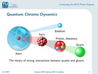
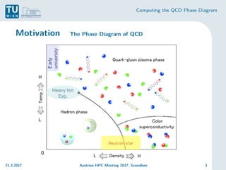
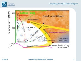
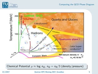
The document discusses the computation of the Quantum Chromodynamics (QCD) phase diagram using effective Polyakov line actions and methods to address the sign problem in lattice QCD. It details the motivations, methodologies, preliminary results, and conclusions drawn from a study conducted during an Austrian HPC meeting in 2017. The work contributes to the understanding of QCD by solving the sign problem and determining effective actions, which may influence future research on quark masses and finite chemical potentials.

1. VIENNA young SCIENTISTS SYMPOSIUM
Computing the QCD Phase Diagram from
Efective Polyakov Line Actions via Relative
Weights and Mean Field Theory
Roman Höllwieserab, Jeff Greensitec
aInstitute of Atomic and Subatomic Physics, Nuclear Physics Dept.,
Vienna University of Technology, Operngasse 9, 1040 Vienna, Austria
bDepartment of Physics, New Mexico State University,
Las Cruces, NM 88003-8001, USA
c Physics and Astronomy Dept., San Francisco State University,
San Francisco, CA 94132, USA

2. Computing the QCD Phase Diagram
Agenda
Motivation
Quantum Chromodynamics (QCD)
Lattice QCD and the Sign problem
The Polyakov Line Action
Preliminary Results
Conclusions & Outlook
Work Group & Collaborations
21.3.2017 Austrian HPC Meeting 2017, Grundlsee 1

3. Computing the QCD Phase Diagram
Quantum Chromo Dynamics
The theory of strong interactions between quarks and gluons
21.3.2017 Austrian HPC Meeting 2017, Grundlsee 2

4. Computing the QCD Phase Diagram
Motivation The Phase Diagram of QCD
21.3.2017 Austrian HPC Meeting 2017, Grundlsee 3

5. Computing the QCD Phase Diagram
The phase Diagram of H2O
21.3.2017 Austrian HPC Meeting 2017, Grundlsee 4

6. Computing the QCD Phase Diagram
21.3.2017 Austrian HPC Meeting 2017, Grundlsee 5

7. Computing the QCD Phase Diagram
Chemical Potential µ ≈ log nQ, nQ = nB/3 (density/pressure)
21.3.2017 Austrian HPC Meeting 2017, Grundlsee 5

8. Computing the QCD Phase Diagram
Lattice QCD
21.3.2017 Austrian HPC Meeting 2017, Grundlsee 6

9. Computing the QCD Phase Diagram
Lattice QCD and the Sign problem
Z =
R
DUDψ̄Dψ e−SYM(U)−SF(U;µ)
21.3.2017 Austrian HPC Meeting 2017, Grundlsee 7

10. Computing the QCD Phase Diagram
Lattice QCD and the Sign problem
Z =
R
DUDψ̄Dψ e−SYM(U)−SF(U;µ)
SF(U; µ) = −
R
d4x ψ̄ M(U; µ) ψ
21.3.2017 Austrian HPC Meeting 2017, Grundlsee 7

11. Computing the QCD Phase Diagram
Lattice QCD and the Sign problem
Z =
R
DUDψ̄Dψ e−SYM(U)−SF(U;µ)
SF(U; µ) = −
R
d4x ψ̄ M(U; µ) ψ
Z =
R
DU e−SYM(U) det M(U; µ)
21.3.2017 Austrian HPC Meeting 2017, Grundlsee 7

12. Computing the QCD Phase Diagram
Lattice QCD and the Sign problem
Z =
R
DUDψ̄Dψ e−SYM(U)−SF(U;µ)
SF(U; µ) = −
R
d4x ψ̄ M(U; µ) ψ
Z =
R
DU e−SYM(U) det M(U; µ)
numerical evaluation of bosonic integral with importance
sampling, Metropolis, HMC Algorithms, MILC
21.3.2017 Austrian HPC Meeting 2017, Grundlsee 7

13. Computing the QCD Phase Diagram
Lattice QCD and the Sign problem
Z =
R
DUDψ̄Dψ e−SYM(U)−SF(U;µ)
SF(U; µ) = −
R
d4x ψ̄ M(U; µ) ψ
Z =
R
DU e−SYM(U) det M(U; µ)
numerical evaluation of bosonic integral with importance
sampling, Metropolis, HMC Algorithms, MILC
observable hOi =
R
DU e−SYM det M O
R
DU e−SYM det M
21.3.2017 Austrian HPC Meeting 2017, Grundlsee 7

14. Computing the QCD Phase Diagram
Lattice QCD and the Sign problem
Z =
R
DUDψ̄Dψ e−SYM(U)−SF(U;µ)
SF(U; µ) = −
R
d4x ψ̄ M(U; µ) ψ
Z =
R
DU e−SYM(U) det M(U; µ)
numerical evaluation of bosonic integral with importance
sampling, Metropolis, HMC Algorithms, MILC
observable hOi =
R
DU e−SYM det M O
R
DU e−SYM det M
lack of γ5-hermiticity, γ5M(µ)γ5 = M†(−µ∗) 6= M†(µ)
21.3.2017 Austrian HPC Meeting 2017, Grundlsee 7

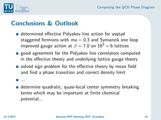
15. Computing the QCD Phase Diagram
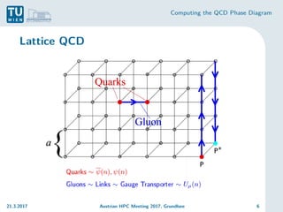
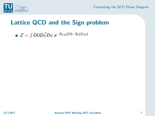
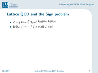
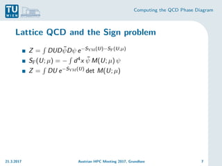
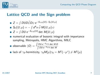
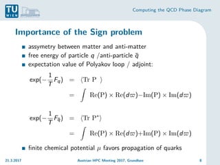
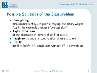
Lattice QCD and the Sign problem
Z =
R
DUDψ̄Dψ e−SYM(U)−SF(U;µ)
SF(U; µ) = −
R
d4x ψ̄ M(U; µ) ψ
Z =
R
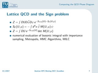
DU e−SYM(U) det M(U; µ)
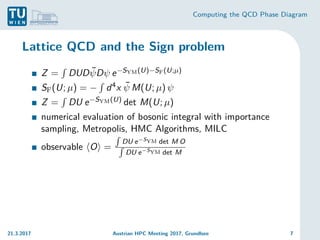
numerical evaluation of bosonic integral with importance
sampling, Metropolis, HMC Algorithms, MILC
observable hOi =
R
DU e−SYM det M O
R
DU e−SYM det M
lack of γ5-hermiticity, γ5M(µ)γ5 = M†(−µ∗) 6= M†(µ)
determinant is complex and satisfies
[det M(µ)]∗ = det M(−µ∗)
21.3.2017 Austrian HPC Meeting 2017, Grundlsee 7

16. Computing the QCD Phase Diagram
Importance of the Sign problem
assymetry between matter and anti-matter
21.3.2017 Austrian HPC Meeting 2017, Grundlsee 8

17. Computing the QCD Phase Diagram
Importance of the Sign problem
assymetry between matter and anti-matter
free energy of particle q /anti-particle q̄
21.3.2017 Austrian HPC Meeting 2017, Grundlsee 8

18. Computing the QCD Phase Diagram
Importance of the Sign problem
assymetry between matter and anti-matter
free energy of particle q /anti-particle q̄
expectation value of Polyakov loop / adjoint:
exp(−
1
T
Fq) = hTr P i
=
Z
Re(P) × Re(d$)−Im(P) × Im(d$)
exp(−
1
T
Fq̄) = hTr P∗
i
=
Z
Re(P) × Re(d$)+Im(P) × Im(d$)
21.3.2017 Austrian HPC Meeting 2017, Grundlsee 8

19. Computing the QCD Phase Diagram
Importance of the Sign problem
assymetry between matter and anti-matter
free energy of particle q /anti-particle q̄
expectation value of Polyakov loop / adjoint:
exp(−
1
T
Fq) = hTr P i
=
Z
Re(P) × Re(d$)−Im(P) × Im(d$)
exp(−
1
T
Fq̄) = hTr P∗
i
=
Z
Re(P) × Re(d$)+Im(P) × Im(d$)
finite chemical potential µ favors propagation of quarks
21.3.2017 Austrian HPC Meeting 2017, Grundlsee 8

20. Computing the QCD Phase Diagram
Possible Solutions of the Sign problem
Reweighting:
measurements of O are given a varying, oscillatory weight
f /g in the ensemble average (“average sign”)
21.3.2017 Austrian HPC Meeting 2017, Grundlsee 9

21. Computing the QCD Phase Diagram
Possible Solutions of the Sign problem
Reweighting:
measurements of O are given a varying, oscillatory weight
f /g in the ensemble average (“average sign”)
Taylor expansion:
of the observable in powers of µ/T at µ = 0
21.3.2017 Austrian HPC Meeting 2017, Grundlsee 9

22. Computing the QCD Phase Diagram
Possible Solutions of the Sign problem
Reweighting:
measurements of O are given a varying, oscillatory weight
f /g in the ensemble average (“average sign”)
Taylor expansion:
of the observable in powers of µ/T at µ = 0
Imaginary µ: analytic continuation of results to real µ
21.3.2017 Austrian HPC Meeting 2017, Grundlsee 9

23. Computing the QCD Phase Diagram
Possible Solutions of the Sign problem
Reweighting:
measurements of O are given a varying, oscillatory weight
f /g in the ensemble average (“average sign”)
Taylor expansion:
of the observable in powers of µ/T at µ = 0
Imaginary µ: analytic continuation of results to real µ
|QCD|:
detM = |detM|eiφ, simulations without eiφ + reweighting
21.3.2017 Austrian HPC Meeting 2017, Grundlsee 9

24. Computing the QCD Phase Diagram
Possible Solutions of the Sign problem
Reweighting:
measurements of O are given a varying, oscillatory weight
f /g in the ensemble average (“average sign”)
Taylor expansion:
of the observable in powers of µ/T at µ = 0
Imaginary µ: analytic continuation of results to real µ
|QCD|:
detM = |detM|eiφ, simulations without eiφ + reweighting
Complex Langevin: stochastic quantization - evolution of
fields in a fictitious time with Brownian noise and search
for stationary solutions with correct measure
21.3.2017 Austrian HPC Meeting 2017, Grundlsee 9

25. Computing the QCD Phase Diagram
Possible Solutions of the Sign problem
Reweighting:
measurements of O are given a varying, oscillatory weight
f /g in the ensemble average (“average sign”)
Taylor expansion:
of the observable in powers of µ/T at µ = 0
Imaginary µ: analytic continuation of results to real µ
|QCD|:
detM = |detM|eiφ, simulations without eiφ + reweighting
Complex Langevin: stochastic quantization - evolution of
fields in a fictitious time with Brownian noise and search
for stationary solutions with correct measure
Worldline formalism and strong coupling limit:
change order of integration, partial integration over loops
and hopping parameter expansion
21.3.2017 Austrian HPC Meeting 2017, Grundlsee 9

26. Computing the QCD Phase Diagram
Effective Polyakov Line Action
Indirect approach: Polyakov line action (SU(3) spin) model
21.3.2017 Austrian HPC Meeting 2017, Grundlsee 10

27. Computing the QCD Phase Diagram
Effective Polyakov Line Action
Indirect approach: Polyakov line action (SU(3) spin) model
fix Polyakov line holonomies U0(~
x, 0) = Ux (temporal
gauge) and integrate out all other d.o.f.
21.3.2017 Austrian HPC Meeting 2017, Grundlsee 10

28. Computing the QCD Phase Diagram
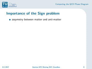
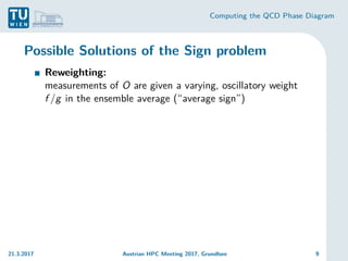
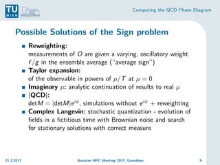
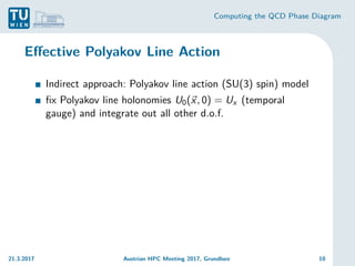
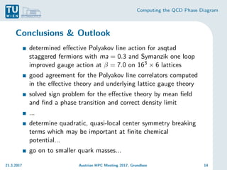
Effective Polyakov Line Action
Indirect approach: Polyakov line action (SU(3) spin) model
fix Polyakov line holonomies U0(~
x, 0) = Ux (temporal
gauge) and integrate out all other d.o.f.
eSP (Ux ) =
R
DU0(~
x, 0)DUkDψ
Q
x δ[Ux − U0(~
x, 0)]eSL
21.3.2017 Austrian HPC Meeting 2017, Grundlsee 10

29. Computing the QCD Phase Diagram
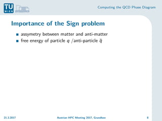
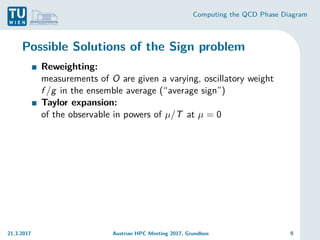
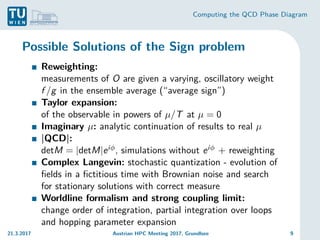
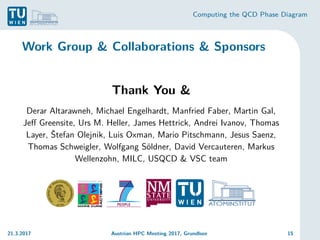
Effective Polyakov Line Action
Indirect approach: Polyakov line action (SU(3) spin) model
fix Polyakov line holonomies U0(~
x, 0) = Ux (temporal
gauge) and integrate out all other d.o.f.
eSP (Ux ) =
R
DU0(~
x, 0)DUkDψ
Q
x δ[Ux − U0(~
x, 0)]eSL
derive SP at µ = 0, for µ > 0 we have (true to all orders of
strong coupling/hopping parameter expansion)
21.3.2017 Austrian HPC Meeting 2017, Grundlsee 10

30. Computing the QCD Phase Diagram
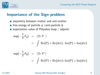
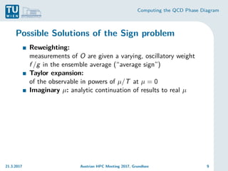
Effective Polyakov Line Action
Indirect approach: Polyakov line action (SU(3) spin) model
fix Polyakov line holonomies U0(~
x, 0) = Ux (temporal
gauge) and integrate out all other d.o.f.
eSP (Ux ) =
R
DU0(~
x, 0)DUkDψ
Q
x δ[Ux − U0(~
x, 0)]eSL
derive SP at µ = 0, for µ > 0 we have (true to all orders of
strong coupling/hopping parameter expansion)
Sµ
P(Ux , U†
x ) = Sµ=0
P [eNt µUx , e−Nt µU†
x ]
21.3.2017 Austrian HPC Meeting 2017, Grundlsee 10

31. Computing the QCD Phase Diagram
Effective Polyakov Line Action
Indirect approach: Polyakov line action (SU(3) spin) model
fix Polyakov line holonomies U0(~
x, 0) = Ux (temporal
gauge) and integrate out all other d.o.f.
eSP (Ux ) =
R
DU0(~
x, 0)DUkDψ
Q
x δ[Ux − U0(~
x, 0)]eSL
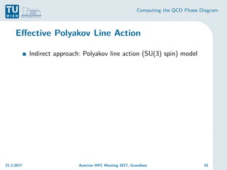
derive SP at µ = 0, for µ > 0 we have (true to all orders of
strong coupling/hopping parameter expansion)
Sµ
P(Ux , U†
x ) = Sµ=0
P [eNt µUx , e−Nt µU†
x ]
hard to compute exp[SP(Ux )], use relative weights...
21.3.2017 Austrian HPC Meeting 2017, Grundlsee 10

32. Computing the QCD Phase Diagram
Preliminary Results
21.3.2017 Austrian HPC Meeting 2017, Grundlsee 11

33. Computing the QCD Phase Diagram
Preliminary Results
21.3.2017 Austrian HPC Meeting 2017, Grundlsee 12

34. Computing the QCD Phase Diagram
Preliminary Results
21.3.2017 Austrian HPC Meeting 2017, Grundlsee 13

35. Computing the QCD Phase Diagram
Conclusions & Outlook
determined effective Polyakov line action for asqtad
staggered fermions with ma = 0.3 and Symanzik one loop
improved gauge action at β = 7.0 on 163 × 6 lattices
21.3.2017 Austrian HPC Meeting 2017, Grundlsee 14

36. Computing the QCD Phase Diagram
Conclusions & Outlook
determined effective Polyakov line action for asqtad
staggered fermions with ma = 0.3 and Symanzik one loop
improved gauge action at β = 7.0 on 163 × 6 lattices
good agreement for the Polyakov line correlators computed
in the effective theory and underlying lattice gauge theory
21.3.2017 Austrian HPC Meeting 2017, Grundlsee 14

37. Computing the QCD Phase Diagram
Conclusions & Outlook
determined effective Polyakov line action for asqtad
staggered fermions with ma = 0.3 and Symanzik one loop
improved gauge action at β = 7.0 on 163 × 6 lattices
good agreement for the Polyakov line correlators computed
in the effective theory and underlying lattice gauge theory
solved sign problem for the effective theory by mean field
and find a phase transition and correct density limit
21.3.2017 Austrian HPC Meeting 2017, Grundlsee 14

38. Computing the QCD Phase Diagram
Conclusions & Outlook
determined effective Polyakov line action for asqtad
staggered fermions with ma = 0.3 and Symanzik one loop
improved gauge action at β = 7.0 on 163 × 6 lattices
good agreement for the Polyakov line correlators computed
in the effective theory and underlying lattice gauge theory
solved sign problem for the effective theory by mean field
and find a phase transition and correct density limit
...
21.3.2017 Austrian HPC Meeting 2017, Grundlsee 14

39. Computing the QCD Phase Diagram
Conclusions & Outlook
determined effective Polyakov line action for asqtad
staggered fermions with ma = 0.3 and Symanzik one loop
improved gauge action at β = 7.0 on 163 × 6 lattices
good agreement for the Polyakov line correlators computed
in the effective theory and underlying lattice gauge theory
solved sign problem for the effective theory by mean field
and find a phase transition and correct density limit
...
determine quadratic, quasi-local center symmetry breaking
terms which may be important at finite chemical
potential...
21.3.2017 Austrian HPC Meeting 2017, Grundlsee 14

40. Computing the QCD Phase Diagram
Conclusions & Outlook
determined effective Polyakov line action for asqtad
staggered fermions with ma = 0.3 and Symanzik one loop
improved gauge action at β = 7.0 on 163 × 6 lattices
good agreement for the Polyakov line correlators computed
in the effective theory and underlying lattice gauge theory
solved sign problem for the effective theory by mean field
and find a phase transition and correct density limit
...
determine quadratic, quasi-local center symmetry breaking
terms which may be important at finite chemical
potential...
go on to smaller quark masses...
21.3.2017 Austrian HPC Meeting 2017, Grundlsee 14

41. Computing the QCD Phase Diagram
Work Group & Collaborations & Sponsors
Thank You &
Derar Altarawneh, Michael Engelhardt, Manfried Faber, Martin Gal,
Jeff Greensite, Urs M. Heller, James Hettrick, Andrei Ivanov, Thomas
Layer, Štefan Olejnik, Luis Oxman, Mario Pitschmann, Jesus Saenz,
Thomas Schweigler, Wolfgang Söldner, David Vercauteren, Markus
Wellenzohn, MILC, USQCD & VSC team
21.3.2017 Austrian HPC Meeting 2017, Grundlsee 15

42. VIENNA young SCIENTISTS SYMPOSIUM
Computing the QCD Phase Diagram from
Efective Polyakov Line Actions via Relative
Weights and Mean Field Theory
Roman Höllwieserab, hroman@kph.tuwien.ac.at
Jeff Greensitec, greensit@sfsu.edu
aInstitute of Atomic and Subatomic Physics, Nuclear Physics Dept.,
Vienna University of Technology, Operngasse 9, 1040 Vienna, Austria
bDepartment of Physics, New Mexico State University,
Las Cruces, NM 88003-8001, USA
c Physics and Astronomy Dept., San Francisco State University,
San Francisco, CA 94132, USA