Pandas.pptx also for analysis of 2 d data

1. 1
Pandas

2. Why pandas?
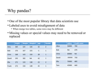
• One of the most popular library that data scientists use
• Labeled axes to avoid misalignment of data
• When merge two tables, some rows may be different
• Missing values or special values may need to be removed or
replaced
height Weight Weight2 age Gender
Amy 160 125 126 32 2
Bob 170 167 155 -1 1
Chris 168 143 150 28 1
David 190 182 NA 42 1
Ella 175 133 138 23 2
Frank 172 150 148 45 1
salary Credit score
Alice 50000 700
Bob NA 670
Chris 60000 NA
David -99999 750
Ella 70000 685
Tom 45000 660

3. Overview
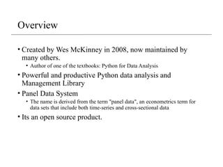
• Created by Wes McKinney in 2008, now maintained by
many others.
• Author of one of the textbooks: Python for Data Analysis
• Powerful and productive Python data analysis and
Management Library
• Panel Data System
• The name is derived from the term "panel data", an econometrics term for
data sets that include both time-series and cross-sectional data
• Its an open source product.

4. Overview - 2
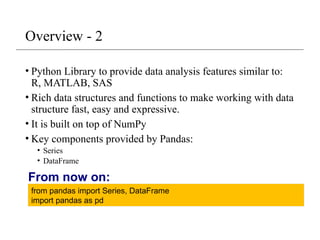
• Python Library to provide data analysis features similar to:
R, MATLAB, SAS
• Rich data structures and functions to make working with data
structure fast, easy and expressive.
• It is built on top of NumPy
• Key components provided by Pandas:
• Series
• DataFrame
from pandas import Series, DataFrame
import pandas as pd
From now on:

5. Series
• One dimensional array-like object
• It contains array of data (of any NumPy data type) with
associated indexes. (Indexes can be strings or integers or
other data types.)
• By default , the series will get indexing from 0 to N where N
= size -1
from pandas import Series, DataFrame
import pandas as pd
obj = Series([4, 7, -5, 3])
print(obj)
print(obj.index)
print(obj.values)
#Output
0 4
1 7
2 -5
3 3
dtype: int64
RangeIndex(start=0, stop=4, step=1)
[ 4 7 -5 3]

6. Series – referencing elements
obj2 = Series([4, 7, -5, 3], index=['d', 'b', 'a', 'c'])
print(obj2)
#Output
d 4
b 7
a -5
c 3
dtype: int64
print(obj2.index)
#Output
Index(['d', 'b', 'a', 'c'], dtype='object')
print(obj2.values)
#Output
[ 4 7 -5 3]
print(obj2['a'])
#Output
-5
obj2['d']= 10
print(obj2[['d', 'c', 'a']])
#Output
d 10
c 3
a -5
dtype: int64
print(obj2[:2])
#Output
d 10
b 7
dtype: int64
print(obj2.a)
#Output
-5

7. Series – array/dict operations
numpy array operations can also be
applied, which will preserve the index-
value link
obj4 = obj3[obj3>0]
print(obj4)
#output
d 4
b 7
c 3
dtype: int64
print(obj3**2)
#output
d 100
b 49
a 25
c 9
dtype: int64
print(‘b’ in obj3)
#output
true
Can be thought of as a dict.
Can be constructed from a dict directly.
obj3 = Series({'d': 4, 'b': 7, 'a': -5, 'c':3 })
print(obj3)
#output
d 4
b 7
a -5
c 3
dtype: int64

8. Series – from dictionary
sdata = {'Texas': 10, 'Ohio': 20, 'Oregon': 15, 'Utah': 18}
states = ['Texas', 'Ohio', 'Oregon', 'Iowa']
obj4 = Series(sdata, index=states)
print(obj4)
#output
Texas 10.0
Ohio 20.0
Oregon 15.0
Iowa NaN
dtype: float64
Missing value
print(pd.isnull(obj4))
#output
Texas False
Ohio False
Oregon False
Iowa True
dtype: bool
print(pd.notnull(obj4))
#output
Texas True
Ohio True
Oregon True
Iowa False
dtype: bool
print(obj4[obj4.notnull()])
#output
Texas 10.0
Ohio 20.0
Oregon 15.0
dtype: float64
dictionary

9. Series – auto alignment
print(obj4.add(obj5))
#output
Iowa NaN
Ohio 40.0
Oregon 30.0
Texas 20.0
Utah NaN
dtype: float64
sdata = {'Texas': 10, 'Ohio': 20, 'Oregon': 15, 'Utah': 18}
states = ['Texas', 'Ohio', 'Oregon', 'Iowa']
obj4 = Series(sdata, index=states)
print(obj4)
#Output
Texas 10.0
Ohio 20.0
Oregon 15.0
Iowa NaN
dtype: float64
sdata = {'Texas': 10, 'Ohio': 20, 'Oregon': 15, 'Utah': 18}
states = ['Texas', 'Ohio', 'Oregon', 'Utah']
obj5 = Series(sdata, index=states)
print(obj5)
#Output
Texas 10
Ohio 20
Oregon 15
Utah 18
dtype: int64

10. Series name and index name
sdata = {'Texas': 10, 'Ohio': 20, 'Oregon': 15, 'Utah': 18}
states = ['Texas', 'Ohio', 'Oregon', 'Iowa']
obj4 = Series(sdata, index=states)
obj4.name = 'population'
obj4.index.name = 'state'
print(obj4)
#output
state
Texas 10.0
Ohio 20.0
Oregon 15.0
Iowa NaN
Name: population, dtype: float64

11. Series name and index name
• Index of a series can be changed to a different index.
obj4.index = ['Florida', 'New York', 'Kentucky', 'Georgia']
Florida 10.0
New York 20.0
Kentucky 15.0
Georgia NaN
Name: population, dtype: float64
• Index object itself is immutable.
obj4.index[2]='California'
TypeError: Index does not support mutable operations
print(obj4.index)
Index(['Florida', 'New York', 'Kentucky', 'Georgia'], dtype='object')

12. Indexing, selection and filtering
• Series can be sliced/accessed with label-based indexes, or
using position-based indexes
S = Series(range(4), index=['zero', 'one', 'two', 'three'])
print(S['two'])
2
print(S[['zero', 'two']])
zero 0
two 2
dtype: int64
print(S[2])
2
print(S[[0,2]])
zero 0
two 2
dtype: int64
list operator for items >1

13. Indexing, selection and filtering
• Series can be sliced/accessed with label-based indexes, or
using position-based indexes
S = Series(range(4), index=['zero', 'one', 'two', 'three'])
print(S[:2])
zero 0
one 1
dtype: int32
print(S['zero': 'two'])
zero 0
one 1
two 2
dtype: int32
Inclusive
print(S[S > 1])
two 2
three 3
dtype: int32
print(S[-2:])
two 2
three 3
dtype: int32

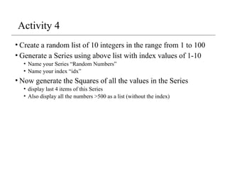
14. Activity 4
• Create a random list of 10 integers in the range from 1 to 100
• Generate a Series using above list with index values of 1-10
• Name your Series “Random Numbers”
• Name your index “idx”
• Now generate the Squares of all the values in the Series
• display last 4 items of this Series
• Also display all the numbers >500 as a list (without the index)

15. DataFrame
• A DataFrame is a tabular data structure comprised of rows and
columns, akin to a spreadsheet or database table.
• It can be treated as an ordered collection of columns
• Each column can be a different data type
• Have both row and column indices
data = {'state': ['Ohio', 'Ohio', 'Ohio', 'Nevada', 'Nevada'],
'year': [2000, 2001, 2002, 2001, 2002],
'pop': [1.5, 1.7, 3.6, 2.4, 2.9]}
frame = DataFrame(data)
print(frame)
#output
state year pop
0 Ohio 2000 1.5
1 Ohio 2001 1.7
2 Ohio 2002 3.6
3 Nevada 2001 2.4
4 Nevada 2002 2.9

16. DataFrame – specifying columns and indices
• Order of columns/rows can be specified.
• Columns not in data will have NaN.
frame2 = DataFrame(data, columns=['year', 'state', 'pop', 'debt'], index=['A', 'B', 'C', 'D', 'E'])
Print(frame2)
year state pop debt
A 2000 Ohio 1.5 NaN
B 2001 Ohio 1.7 NaN
C 2002 Ohio 3.6 NaN
D 2001 Nevada 2.4 NaN
E 2002 Nevada 2.9 NaN
Same order
Initialized with NaN

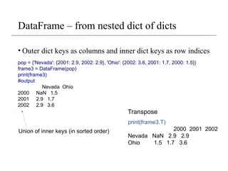
17. DataFrame – from nested dict of dicts
• Outer dict keys as columns and inner dict keys as row indices
pop = {'Nevada': {2001: 2.9, 2002: 2.9}, 'Ohio': {2002: 3.6, 2001: 1.7, 2000: 1.5}}
frame3 = DataFrame(pop)
print(frame3)
#output
Nevada Ohio
2000 NaN 1.5
2001 2.9 1.7
2002 2.9 3.6
print(frame3.T)
2000 2001 2002
Nevada NaN 2.9 2.9
Ohio 1.5 1.7 3.6
Transpose
Union of inner keys (in sorted order)

18. DataFrame – index, columns, values
frame3.index.name = 'year'
frame3.columns.name='state‘
print(frame3)
state Nevada Ohio
year
2000 NaN 1.5
2001 2.9 1.7
2002 2.9 3.6
print(frame3.index)
Int64Index([2000, 2001, 2002], dtype='int64', name='year')
print(frame3.columns)
Index(['Nevada', 'Ohio'], dtype='object', name='state')
print(frame3.values)
[[nan 1.5]
[2.9 1.7]
[2.9 3.6]]

19. DataFrame – retrieving a column
• A column in a DataFrame can be retrieved as a Series by
dict-like notation or as attribute
data = {'state': ['Ohio', 'Ohio', 'Ohio', 'Nevada', 'Nevada'],
'year': [2000, 2001, 2002, 2001, 2002],
'pop': [1.5, 1.7, 3.6, 2.4, 2.9]}
frame = DataFrame(data)
print(frame['state'])
0 Ohio
1 Ohio
2 Ohio
3 Nevada
4 Nevada
Name: state, dtype: object
print(frame.state)
0 Ohio
1 Ohio
2 Ohio
3 Nevada
4 Nevada
Name: state, dtype: object

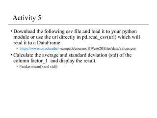
20. Activity 5
• Download the following csv file and load it to your python
module or use the url directly in pd.read_csv(url) which will
read it to a DataFrame
• https://www.cs.odu.edu/~sampath/courses/f19/cs620/files/data/values.csv
• Calculate the average and standard deviation (std) of the
column factor_1 and display the result.
• Pandas mean() and std()

21. DataFrame – getting rows
• loc for using indexes and iloc for using positions
• loc gets rows (or columns) with particular labels from the index.
• iloc gets rows (or columns) at particular positions in the index (so it only takes integers).
data = {'state': ['Ohio', 'Ohio', 'Ohio', 'Nevada', 'Nevada'],
'year': [2000, 2001, 2002, 2001, 2002],
'pop': [1.5, 1.7, 3.6, 2.4, 2.9]}
frame2 = DataFrame(data, columns=['year', 'state', 'pop', 'debt'], index=['A', 'B', 'C', 'D', 'E'])
print(frame2)
year state pop debt
A 2000 Ohio 1.5 NaN
B 2001 Ohio 1.7 NaN
C 2002 Ohio 3.6 NaN
D 2001 Nevada 2.4 NaN
E 2002 Nevada 2.9 NaN
print(frame2.loc['A'])
year 2000
state Ohio
pop 1.5
debt NaN
Name: A, dtype: object
print(frame2.loc[['A', 'B']])
year state pop debt
A 2000 Ohio 1.5 NaN
B 2001 Ohio 1.7 NaN
print(frame2.loc['A':'E',
['state','pop']])
state pop
A Ohio 1.5
B Ohio 1.7
C Ohio 3.6
D Nevada 2.4
E Nevada 2.9
print(frame2.iloc[1:3])
year state pop debt
B 2001 Ohio 1.7 NaN
C 2002 Ohio 3.6 NaN
print(frame2.iloc[:,1:3])
state pop
A Ohio 1.5
B Ohio 1.7
C Ohio 3.6
D Nevada 2.4
E Nevada 2.9

22. DataFrame – modifying columns
frame2['debt'] = 0
print(frame2)
year state pop debt
A 2000 Ohio 1.5 0
B 2001 Ohio 1.7 0
C 2002 Ohio 3.6 0
D 2001 Nevada 2.4 0
E 2002 Nevada 2.9 0
frame2['debt'] = range(5)
print(frame2)
year state pop debt
A 2000 Ohio 1.5 0
B 2001 Ohio 1.7 1
C 2002 Ohio 3.6 2
D 2001 Nevada 2.4 3
E 2002 Nevada 2.9 4
val = Series([10, 10, 10], index = ['A', 'C', 'D'])
frame2['debt'] = val
print(frame2)
year state pop debt
A 2000 Ohio 1.5 10.0
B 2001 Ohio 1.7 NaN
C 2002 Ohio 3.6 10.0
D 2001 Nevada 2.4 10.0
E 2002 Nevada 2.9 NaN
Rows or individual elements can be
modified similarly. Using loc or iloc.

23. DataFrame – removing columns
del frame2['debt']
print(frame2)
year state pop
A 2000 Ohio 1.5
B 2001 Ohio 1.7
C 2002 Ohio 3.6
D 2001 Nevada 2.4
E 2002 Nevada 2.9

24. Removing rows/columns
print(frame)
c1 c2 c3
r1 0 1 2
r2 3 4 5
r3 6 7 8
print(frame.drop(['r1']))
c1 c2 c3
r2 3 4 5
r3 6 7 8
print(frame.drop(['r1','r3']))
c1 c2 c3
r2 3 4 5
print(frame.drop(['c1'], axis=1))
c2 c3
r1 1 2
r2 4 5
r3 7 8
This returns a new object

25. Reindexing
• Alter the order of rows/columns of a DataFrame or order of a
series according to new index
frame2 = frame.reindex(columns=['c2', 'c3', 'c1'])
print(frame2)
c2 c3 c1
r1 1 2 0
r2 4 5 3
r3 7 8 6
frame2 = frame.reindex(['r1', 'r3', 'r2', 'r4'])
c1 c2 c3
r1 0.0 1.0 2.0
r3 6.0 7.0 8.0
r2 3.0 4.0 5.0
r4 NaN NaN NaN
This returns a new object

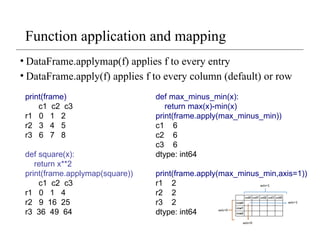
26. Function application and mapping
• DataFrame.applymap(f) applies f to every entry
• DataFrame.apply(f) applies f to every column (default) or row
def max_minus_min(x):
return max(x)-min(x)
print(frame.apply(max_minus_min))
c1 6
c2 6
c3 6
dtype: int64
print(frame.apply(max_minus_min,axis=1))
r1 2
r2 2
r3 2
dtype: int64
print(frame)
c1 c2 c3
r1 0 1 2
r2 3 4 5
r3 6 7 8
def square(x):
return x**2
print(frame.applymap(square))
c1 c2 c3
r1 0 1 4
r2 9 16 25
r3 36 49 64

27. Other DataFrame functions
• sort_index()
frame.index=['A', 'C', 'B'];
frame.columns=['b','a','c'];
print(frame)
b a c
A 0 1 2
C 3 4 5
B 6 7 8
print(frame.sort_index())
b a c
A 0 1 2
B 6 7 8
C 3 4 5
print(frame.sort_index(axis=1))
a b c
A 1 0 2
C 4 3 5
B 7 6 8
frame = DataFrame(np.random.randint(0, 10,
9).reshape(3,-1), index=['r1', 'r2', 'r3'], columns=['c1', 'c2',
'c3'])
print(frame)
c1 c2 c3
r1 6 9 0
r2 8 2 9
r3 8 0 6
print(frame.sort_values(by='c1'))
c1 c2 c3
r1 6 9 0
r2 8 2 9
r3 8 0 6
print(frame.sort_values(axis=1,by=['r3','r1']))
c2 c3 c1
r1 9 0 6
r2 2 9 8
r3 0 6 8
• sort_values()

28. Other DataFrame functions
• mean()
• Mean(axis=0, skipna=True)
• sum()
• cumsum()
• describe(): return summary statistics of each column
• for numeric data: mean, std, max, min, 25%, 50%, 75%, etc.
• For non-numeric data: count, uniq, most-frequent item, etc.
• corr(): correlation between two Series, or between columns
of a DataFrame
• corr_with(): correlation between columns of DataFram and a
series or between the columns of another DataFrame

29. Handling missing data
• Filtering out missing values
from numpy import nan as NaN
data = Series([1, NaN, 2.5, NaN, 6])
print(data)
0 1.0
1 NaN
2 2.5
3 NaN
4 6.0
dtype: float64
print(data.notnull())
0 True
1 False
2 True
3 False
4 True
dtype: bool
print(data[data.notnull()])
0 1.0
2 2.5
4 6.0
dtype: float64
print(data.dropna())
0 1.0
2 2.5
4 6.0
dtype: float64

30. Handling missing data - 2
data = DataFrame([[1, 2, 3], [1, NaN, NaN], [NaN, NaN, NaN], [NaN, 4, 5]])
print(data)
0 1 2
0 1.0 2.0 3.0
1 1.0 NaN NaN
2 NaN NaN NaN
3 NaN 4.0 5.0
print(data.dropna())
0 1 2
0 1.0 2.0 3.0
print(data.dropna(how='all'))
0 1 2
0 1.0 2.0 3.0
1 1.0 NaN NaN
3 NaN 4.0 5.0
print(data.dropna(axis=1, how='all'))
0 1 2
0 1.0 2.0 3.0
1 1.0 NaN NaN
2 NaN NaN NaN
3 NaN 4.0 5.0
data[4]=NaN
print(data)
0 1 2 4
0 1.0 2.0 3.0 NaN
1 1.0 NaN NaN NaN
2 NaN NaN NaN NaN
3 NaN 4.0 5.0 NaN
print(data.dropna(axis=1, how='all'))
0 1 2
0 1.0 2.0 3.0
1 1.0 NaN NaN
2 NaN NaN NaN
3 NaN 4.0 5.0

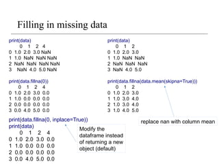
31. Filling in missing data
print(data)
0 1 2 4
0 1.0 2.0 3.0 NaN
1 1.0 NaN NaN NaN
2 NaN NaN NaN NaN
3 NaN 4.0 5.0 NaN
print(data.fillna(0))
0 1 2 4
0 1.0 2.0 3.0 0.0
1 1.0 0.0 0.0 0.0
2 0.0 0.0 0.0 0.0
3 0.0 4.0 5.0 0.0
print(data.fillna(0, inplace=True))
print(data)
0 1 2 4
0 1.0 2.0 3.0 0.0
1 1.0 0.0 0.0 0.0
2 0.0 0.0 0.0 0.0
3 0.0 4.0 5.0 0.0
print(data)
0 1 2
0 1.0 2.0 3.0
1 1.0 NaN NaN
2 NaN NaN NaN
3 NaN 4.0 5.0
print(data.fillna(data.mean(skipna=True)))
0 1 2
0 1.0 2.0 3.0
1 1.0 3.0 4.0
2 1.0 3.0 4.0
3 1.0 4.0 5.0
Modify the
dataframe instead
of returning a new
object (default)
replace nan with column mean