The document outlines various methods for creating data frames in Python using libraries like pandas, including from dictionaries of series, dictionaries of dictionaries, and numpy ndarrays. It also discusses techniques for selecting, adding, deleting, exploring, and analyzing data frames, along with interoperability between data frames and numpy functions. The detailed examples provided demonstrate how to manipulate and visualize data effectively.

2.  Creating a Data Frame from a Dict of Series: You can create a Data Frame
by passing a dictionary of Series objects, where the keys of the dictionary will
become the column names of the Data Frame.
 Each Series in the dictionary must have the same length.
 For example:
data = {'A': pd.Series([1, 2, 3]), 'B': pd.Series([4, 5, 6])}
df = pd.DataFrame(data)
 Creating a Data Frame from a Dict of Dicts: You can also create a Data
Frame by passing a dictionary of dictionaries, where the outer dictionary keys
become the column names and the inner dictionary keys become the row index.
 For example:
data = {'A': {'a1': 1, 'a2': 2, 'a3': 3}, 'B': {'a1': 4, 'a2': 5, 'a3': 6}}
df = pd.DataFrame(data)
 In both cases, the resulting Data Frame will have the dictionary keys as the
column names and the common index from the Series or inner dictionaries as
the row index.

3.  Create a Data Frame in Python from a dictionary of NumPy ndarrays (Ndimensional
arrays). Here are the key points:Creating a Data Frame from a Dict of Ndarrays:You can
create a Data Frame by passing a dictionary of NumPy ndarray objects, where the keys of
the dictionary will become the column names of the Data Frame.
 Each ndarray in the dictionary must have the same length.
 For example:
data = {'A': np.array([1, 2, 3]), 'B': np.array([4, 5, 6])}
df = pd.DataFrame(data)
 In this case, the resulting Data Frame will have the dictionary keys as the column names
and the common length of the ndarrays as the row index.The key difference from creating
a Data Frame from a dictionary of Series or dictionaries is that here you are using NumPy
ndarrays instead of Python builtin data structures like Series or dictionaries.

4.  Creating a Data Frame from a Structured or Record Array:You can create a Data Frame
directly from a NumPy structured or record array.
 A structured array is a special type of NumPy ndarray where each element is a row and
the columns are defined by the data types specified when creating the array.
 For example:
import numpy as np
Create a structuredarray data = np.array([('Alex', 10), ('Bob', 12), ('Clarke', 13)],
dtype=[('Name', 'U10'), ('Age', int)])
Create a Data Frame from the structured array
df = pd.DataFrame(data)
 In this case, the resulting Data Frame will have the field names from the structured array
as the column names, and each row will correspond to an element in the structured array.
 The key advantage of creating a Data Frame from a structured array is that the column
names and data types are automatically inferred from the array definition, making it a
convenient way to convert structured data into a tabular format.

5. Creating a Data Frame from a List of Dicts:
You can create a Data Frame by passing a list of dictionaries, where each dictionary
represents a row and the keys of the dictionaries become the column names of the Data
Frame.
For example:
data = [{'A': 1, 'B': 4}, {'A': 2, 'B': 5}, {'A': 3, 'B': 6}]
df = pd.DataFrame(data)
In this case, the resulting Data Frame will have the keys from the dictionaries as the column
names, and each row will correspond to a dictionary in the list.
The keys from the first dictionary in the list are used to determine the column names. If other
dictionaries in the list have different keys, they will be included as columns with NaN values
where data is missing.
This method is useful when you have data stored in a list of dictionaries, as it allows you to
easily convert it into a tabular Data Frame format for further analysis and manipulation.

6. Creating Data Frames from a Dict of Tuples
You can create a Data Frame in Python from a dictionary where the values are tuples, and
the keys become the column names.
For example:
data = {'A': (1, 2, 3), 'B': (4, 5, 6)}
df = pd.DataFrame(data)
In this case, the resulting Data Frame will have the dictionary keys as the column names, and
the length of the tuples will determine the number of rows.

7. Selecting Data Frames
You can select data from a Data Frame in various ways:
By column name: `df['A']` or `df.A`
By row position: `df.iloc` (first row)
By row label: `df.loc['row_label']`
By boolean indexing: `df[df['A'] > 2]
You can also select multiple columns or rows using lists, slices, and boolean conditions:
Select multiple columns: `df[['A', 'B']]`
Select rows by position: `df.iloc[0:2]`
Select rows by label: `df.loc['row1':'row3']`
Select rows by boolean condition: `df[df['A'] > 2 & df['B'] < 6]`
The key is to use the appropriate selection method (by position, label, or boolean condition)
to extract the desired data from the Data Frame.

8. Adding and Deleting Data Frame Columns
To add a new column to a Data Frame:
Assign a Series or scalar value to a new column name
`df['C'] = df['A'] * df['B']`
`df['D'] = 0`
Use the `assign()` method to create new columns
`df = df.assign(C=df['A'] * df['B'], D=0)`
To delete columns from a Data Frame:
Drop columns by name or index
`df = df.drop('A', axis=1)`
`df = df.drop(df.columns[[0, 1]], axis=1)`
Assign `None` to delete a column inplace
`df['A'] = None`
`del df['B']`
The `axis=1` argument specifies that the operation should be applied to columns.

9. Assigning New Columns in Method Chains
You can assign new columns to a Data Frame using method chaining. This allows you to
create new columns and perform other operations in a single statement.
Example:
df = df.assign(C=df['A'] * df['B'], D=0)
In this example, a new column 'C' is created by multiplying columns 'A' and 'B', and a new
column 'D' is created with a constant value of 0.

10. Row Selection
By position using `df.iloc`:
`df.iloc` Select first row
`df.iloc[0:2]` Select first two rows
By label using `df.loc`:
`df.loc['row1']` Select row with label 'row1'
`df.loc['row1':'row3']` Select rows with labels 'row1' to 'row3‘
By boolean indexing:
`df[df['A'] > 2]` Select rows where column 'A' is greater than 2

11.  Row Addition
 Append a Series or DataFrame using `df.append()`:
 `df = df.append({'A': 4, 'B': 7}, ignore_index=True)`
 Concatenate DataFrames using `pd.concat()`:
 `df2 = pd.DataFrame({'A': , 'B': })`
 `df = pd.concat([df, df2], ignore_index=True)`

12. Row Deletion:
Drop rows by position using `df.drop()`:
`df = df.drop(df.index)`
Delete first row
`df = df.drop(df.index[0:2])`
Delete first two rows
Drop rows by label using `df.loc[]` and `df.drop()`:
`df = df.drop(df.loc[df['A'] < 2].index)`
Delete rows where 'A' is less than 2
The key is to use the appropriate row selection method (by position, label, or boolean
condition) to identify the rows you want to delete.

13. Exploring and analyzing a Data Frame in Python involves several techniques to understand
and manipulate the data. Here are some key methods:
Exploring a Data Frame
1. Basic Information:
- Use the `info()` method to get basic information about the Data Frame, including the
number of rows and columns, data types, and memory usage.
- Example:
df.info()

14. 2. Data Types:
- Use the `dtypes` attribute to see the data types of each column.
- Example:
df.dtypes
3. Head and Tail:
- Use the `head()` and `tail()` methods to view the first and last few rows of the Data
Frame.
- Example:
df.head()
df.tail()

15. 4. Descriptive Statistics:
- Use the `describe()` method to get descriptive statistics such as mean, standard deviation,
minimum, and maximum for each column.
- Example:
df.describe()

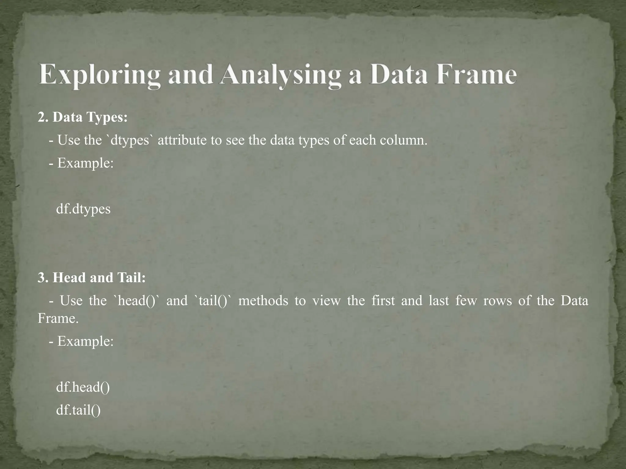
16. Analyzing a Data Frame
1. Grouping and Aggregating:
- Use the `groupby()` method to group the data by one or more columns and apply
aggregations such as `sum`, `mean`, `max`, etc.
- Example:
grouped_df = df.groupby('column_name').sum()
2. Filtering:
- Use boolean indexing to filter rows based on conditions.
- Example:
filtered_df = df[df['column_name'] > 5]

17. 3. Sorting:
- Use the `sort_values()` method to sort the Data Frame by one or more columns.
- Example:
sorted_df = df.sort_values(by='column_name')
4. Plotting:
- Use plotting libraries such as `matplotlib` and `seaborn` to visualize the data.
- Example:
import matplotlib.pyplot as plt
plt.plot(df['column_name'], df['other_column'])
plt.show()

18. 5. Data Manipulation:
- Use methods like `drop()`, `dropna()`, `fillna()`, `rename()`, and `reset_index()` to
manipulate the Data Frame.
- Example:
df.drop('column_name', axis=1, inplace=True)
Example
Here is a complete example of exploring and analyzing a Data Frame:
import pandas as pd
import matplotlib.pyplot as plt

19. #Create a sample Data Frame
data = {'A': [1, 2, 3, 4, 5],
'B': [4, 5, 6, 7, 8],
'C': [7, 8, 9, 10, 11]}
df = pd.DataFrame(data)
#Basic Information
print(df.info())
#Data Types
print(df.dtypes)
#Head and Tail
print(df.head())
print(df.tail())

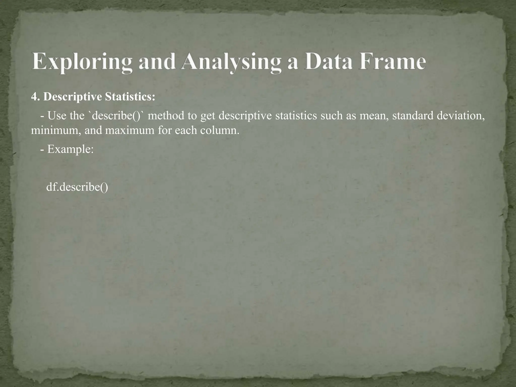
20. #Descriptive Statistics
print(df.describe())
#Grouping and Aggregating
grouped_df = df.groupby('A').sum()
print(grouped_df)
#Filtering
filtered_df = df[df['B'] > 5]
print(filtered_df)
#Sorting
sorted_df = df.sort_values(by='B')
print(sorted_df)

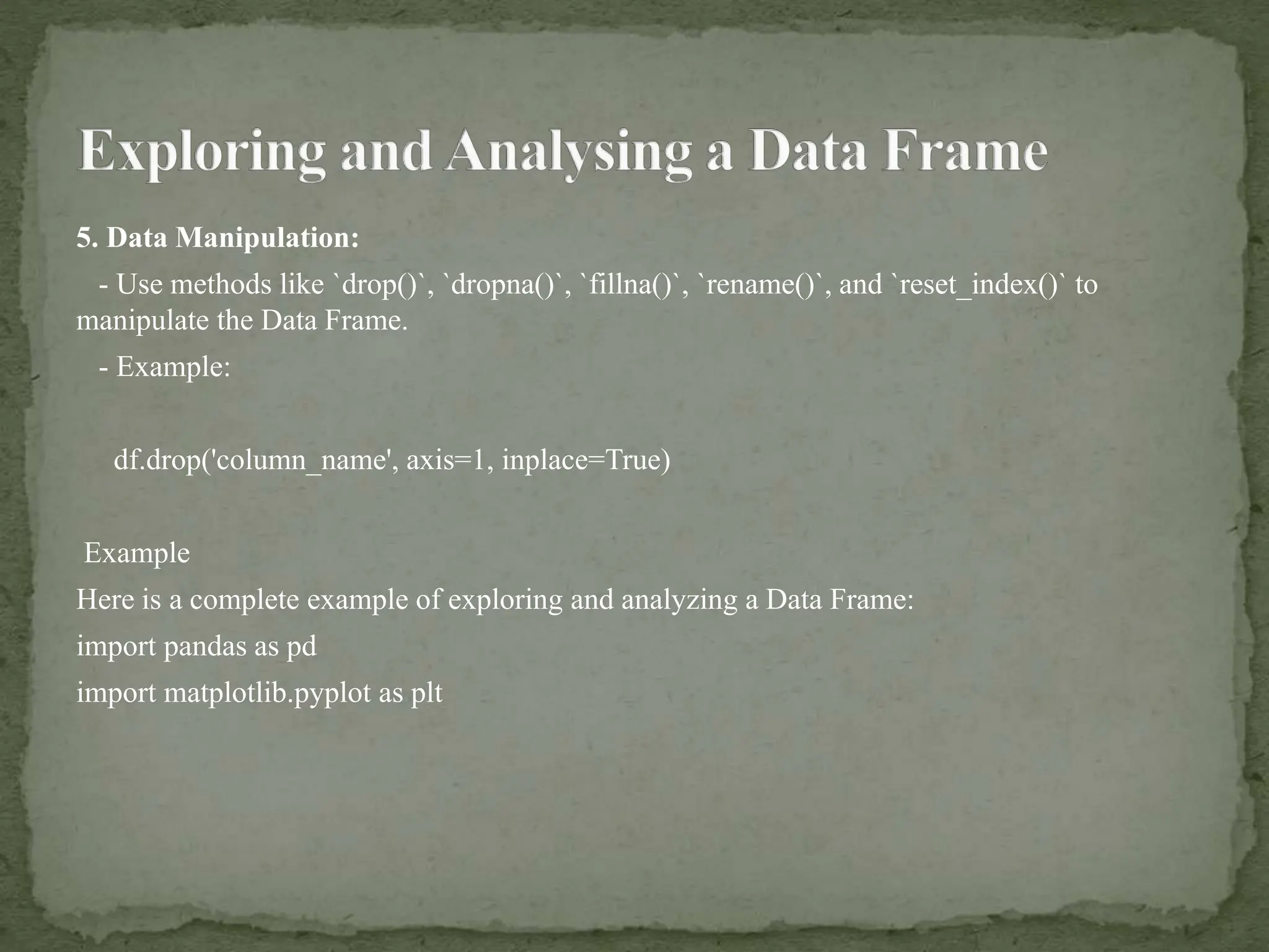
21. #Plotting
plt.plot(df['A'], df['B'])
plt.show()
#Data Manipulation
df.drop('C', axis=1, inplace=True)
print(df)
This example demonstrates how to explore and analyze a Data Frame by getting basic
information, checking data types, viewing the first and last few rows, calculating descriptive
statistics, grouping and aggregating data, filtering rows, sorting data, plotting data, and
manipulating the Data Frame.

22. Indexing and Selecting Data Frames
1. Selecting Columns:
- Access columns by name using square brackets `df['column_name']` or dot notation
`df.column_name`.
- Select multiple columns using a list of column names `df[['col1', 'col2']]`.

23. 2. Selecting Rows:
- By position using `df.iloc`:
- `df.iloc` # Select first row
- `df.iloc[0:2]` # Select first two rows
- By label using `df.loc`:
- `df.loc['row1']` # Select row with label 'row1'
- `df.loc['row1':'row3']` # Select rows with labels 'row1' to 'row3'
- By boolean indexing:
- `df[df['column_name'] > 2]` # Select rows where 'column_name' is greater than 2.
3. Selecting Rows and Columns:
- Combine row and column selection:
- `df.loc['row1', 'column_name']` # Select value at row 'row1', column 'column_name'
- `df.iloc[0, 1]` # Select value at row 0, column 1 (by position)

24. 4. Transposing a Data Frame:
- Use the `T` attribute to transpose the Data Frame:
- `df_transposed = df.T.
5. Interoperability with NumPy:
- You can use NumPy functions directly on a Data Frame:
- `df.sum()` # Apply NumPy's sum() function to the Data Frame
- `df.values` # Access the underlying NumPy array.
The key is to use the appropriate indexing method (by position, label, or boolean condition)
to select the desired rows and columns from the Data Frame. The flexibility of Data Frame
indexing allows you to extract specific subsets of the data for further analysis and
manipulation.

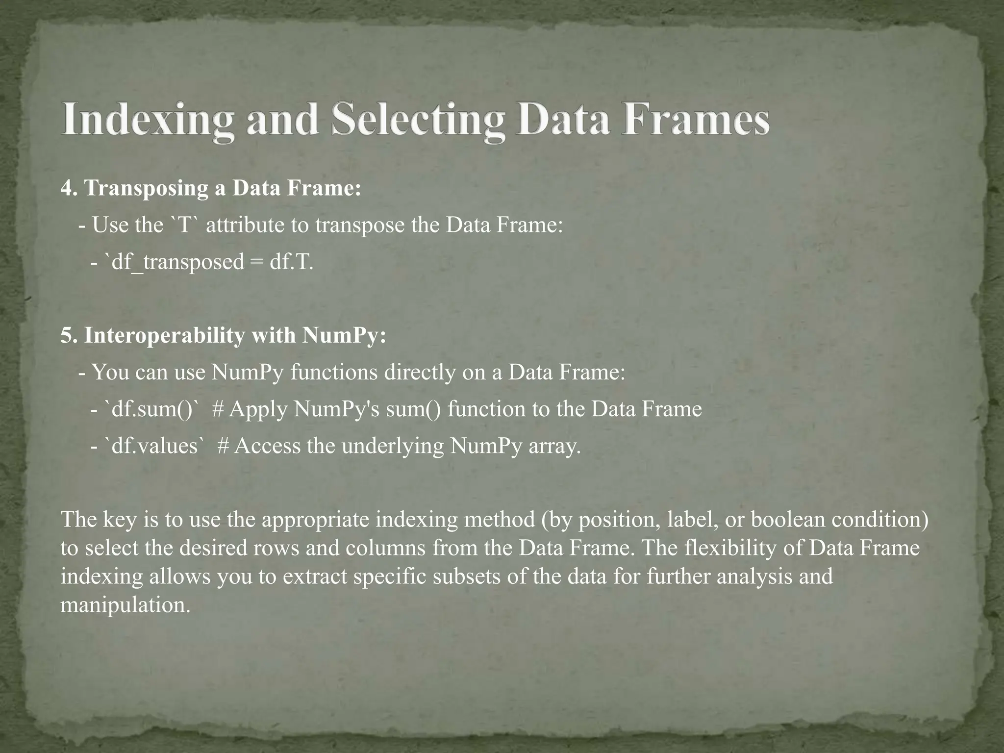
25. Transposing a Data Frame
You can transpose a Data Frame using the `T` attribute:
- `df_transposed = df.T`[170]
This will swap the rows and columns of the Data Frame, effectively transposing it.
Data Frame Interoperability with NumPy Functions
You can use NumPy functions directly on a Data Frame:
- `df.sum()` # Apply NumPy's sum() function to the Data Frame
- `df.values` # Access the underlying NumPy array[171]

26. This allows you to leverage the powerful functionality of NumPy's numerical
operations and access the underlying data representation when working with Data
Frames.
Some key points:
- You can apply NumPy functions like `sum()`, `mean()`, `std()`, etc. directly on a
Data Frame.
- The `values` attribute of a Data Frame returns the underlying NumPy ndarray,
allowing you to access the raw data.
- This interoperability between Data Frames and NumPy makes it easy to perform
advanced numerical and statistical analysis on tabular data.
By using these techniques, you can seamlessly transition between the high-level
abstraction of Data Frames and the low-level control of NumPy arrays when working
with data in Python.