Download to read offline

![Measuring relative phase between oscilloscope traces using the Lissajous
(ellipse) method
Requirements:
Oscilloscope:
• Able to display the voltage of one channel vertically and
the other channel horizontally.
(Includes virtually all oscilloscopes.)
Waveforms:
• Sinusoidal
• Common frequency
Method:
• Set the oscilloscope to xy mode.
• Scale each voltage channel so that the ellipse fits in the display.
(This may be a line if the phase difference is near 0° or 180°.)
• Ground or zero each channel separately and adjust the line to the
center (vertical or horizontal) axis of the display. (On analog
scopes, you can ground both simultaneously and center the
resulting dot.)
• Return to ac coupling to display the ellipse.
• (Optional) If you can continuously adjust the voltage per division,
scale your waveforms to an even number of divisions. You can
then center the ellipse more accurately by positioning the
waveform between gridlines on the display.
• Measure the horizontal width A and zero crossing width C as
shown in the figure to the right.
• The magnitude of the phase difference is then given by
( )
( )[ ]⎩
⎨
⎧
−°±
±
=θ−θ −
−
QIIinellipseoftop/sin180
QIinellipseoftop/sin
1
1
12
AC
AC
• The sign of ( )12 θ−θ must be determined by inspection of the
dual-channel trace.
Figure 2. Lissajous
figure. (by Paul Kavan)](https://image.slidesharecdn.com/oscilloscopetutorial-phasemeasurement-180516041851/85/Oscilloscope-tutorial-phasemeasurement-3-320.jpg)
![Explanation:
Given two waveforms:
v1 vertical, v2 horizontal
( ) ( )
( ) ( )222
111
cos
cos
θ+ω=
θ+ω=
tVtv
tVtv
p
p
The ellipse will cross the horizontal axis at
time t0 when v1(t0) = 0 or ⎥
⎦
⎤
⎢
⎣
⎡
θ−π⎟
⎠
⎞
⎜
⎝
⎛
+
ω
=⇒π⎟
⎠
⎞
⎜
⎝
⎛
+=θ+ω 1010
2
11
2
1
ntnt
At this time the value of v2(t0) will be
( ) ⎥
⎦
⎤
⎢
⎣
⎡
θ+θ−π⎟
⎠
⎞
⎜
⎝
⎛
+= 21202
2
1
cos nVtv p
A trig identity yields*
( ) βα−βα=β+α sinsincoscoscos
( ) ( )
⎩
⎨
⎧
−
+
θ−θ±=
evenisif
oddisif
sin 12
above
/
2
02
n
n
V
tv
AC
p
321
Now we have two nasty details to take care of.
• First, we have to be careful taking the inverse sine, since a phase change between 90° and
180° gives rise to the same (C / A) ratio as its coangle.
To decide which we have, find the times tp1
and tp2 when v1(t) and v2(t) peak: ω
θ
−=⇒=θ+ω 1
111 0 pp tt
And look at ( )tv2 at that time: ( ) ( )12212 cos θ−θ= pp Vtv
Conversely ( ) ( ) ( )12121121 coscos θ−θ=θ−θ= ppp VVtv
So if v2 is positive when v1 is maximum positive if |θ2 − θ1| is between 0° and 90°. For
this case, the top and right side of the ellipse will be in Quadrant I.
But if v2 is negative when v1 maximum positive, then we need the other angle with the
same sine. This means the top of the ellipse will be in Quadrant II and the right side in
Quadrant IV. So if °>θ−θ 9012 , then the actual inverse sine is ( )[ ]AC /sin180 1−
−° ,
where sin-1
represents the principle inverse sine between 0° and 90°.
• Second, what is the sign of ( )12 θ−θ ?
Suppose we have a case where two voltages
( )tv 1' and ( )tv 2' have the same amplitudes
as before but with opposite phase angles:
( ) ( )
( ) ( )222
111
cos'
cos'
θ−ω=
θ−ω=
tVtv
tVtv
p
p
Since ( ) ( ),coscos α−=α ( ) ( )[ ]
( ) ( )[ ]222
111
cos'
cos'
θ+−ω=
θ+−ω=
tVtv
tVtv
p
p
This is the exact same as ( )tv1 and ( )tv2 , but reversed in time. The Lissajous figure will
look exactly the same, but the trace will precess in the opposite direction. That means the
sign of the phase difference cannot be determined in xy mode.
So we need the dual-channel trace to determine the sign of ( )12 θ−θ .](https://image.slidesharecdn.com/oscilloscopetutorial-phasemeasurement-180516041851/85/Oscilloscope-tutorial-phasemeasurement-4-320.jpg)
![Measuring relative phase between oscilloscope traces using the product
method
Requirements:
Oscilloscope:
• Automatic amplitude measurement (preferably rms
value) for each channel.
• Display the product of the two channels and calculate its
dc offset automatically.
This method was developed using the Tektronix 2012B oscilloscope.
Waveforms:
• Sinusoidal
• Common frequency
Method:
• Display the two traces in voltage v. time mode, along with the product trace in voltage2
v.
time mode. Use ac coupling.
• Fit the traces in the screen vertically.
• Display the MEAN value (dc offset vmath,dc) of the product trace. Show about 10 of its
periods to ensure that the calculation is not affected by partial waveforms at the beginning
and end of the trace. You may also want to average the sampling to reduce error.
• Display the rms amplitude of each of the channels (V1rms and V2rms). Using rms (rather than
peak-to-peak) means that the scope has averaged over the waveform.
• The phase difference is then*
( )
pppp
dcmath
pp
dcmath
rmsrms
dcmath
VV
v
VV
v
VV
v
−−
===θ−θ
21
,
21
,
21
,
12
82
cos
• The sign of ( )12 θ−θ still has to be determined by inspection of the dual-channel trace.
Explanation:
Given two waveforms: ( ) ( )
( ) ( )222
111
cos
cos
θ+ω=
θ+ω=
tVtv
tVtv
p
p
Their product is ( ) ( ) ( )2121 coscos θ+ωθ+ω= ttVVtv ppmath
Applying the trig identity ( ) ( )
2
coscos
coscos
β−α+β+α
=βα
yields
( ) ( ) ( )[ ]2121
21
2coscos
2
θ+θ+ω+θ−θ= t
VV
tv pp
math
The phase difference determines the dc
offset of the math trace: ( )21
21
, cos
2
θ−θ=
pp
dcmath
VV
v
*This method is least precise when the phase difference is nearly 0° or 180°, cases where cosθ is
not sensitive to θ.](https://image.slidesharecdn.com/oscilloscopetutorial-phasemeasurement-180516041851/85/Oscilloscope-tutorial-phasemeasurement-5-320.jpg)
![Figure 3. Oscilloscope display for the product method showing the dual-channel display and the
product trace, along with the values for V1rms, V2rms, and vmath,dc as calculated by the oscilloscope.
Here ( )[ ] °=⋅=θ−θ −
5.78294.082.1/107.0cos 1
12 . Since the peak in channel 2 is to the left of
the peak in channel 1, v2 leads v1.
Figure 4. Spreadsheet used for curvefitting method. Regions are color coded according to
function: instructions, preference, data, results, error figure (between guess and experiment),
parameter guesses (calculated from data), fit parameters. Approximate values of the fit
parameters must supplied before using the Solve function.](https://image.slidesharecdn.com/oscilloscopetutorial-phasemeasurement-180516041851/85/Oscilloscope-tutorial-phasemeasurement-6-320.jpg)


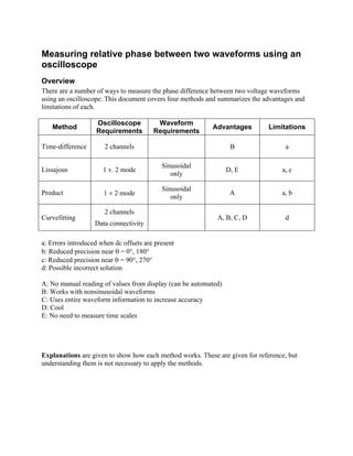
This document describes four methods for measuring the relative phase between two waveforms using an oscilloscope: time-difference, Lissajous, product, and curvefitting. It provides the requirements, steps, advantages, and limitations of each method. The time-difference and Lissajous methods work for sinusoidal waveforms, while product and curvefitting can handle nonsinusoidal waveforms. Curvefitting uses the entire waveform information to increase accuracy.


