Download to read offline
![9
Vol.:(0123456789)
Scientific Reports | (2024) 14:13354 | https://doi.org/10.1038/s41598-024-64234-x
www.nature.com/scientificreports/
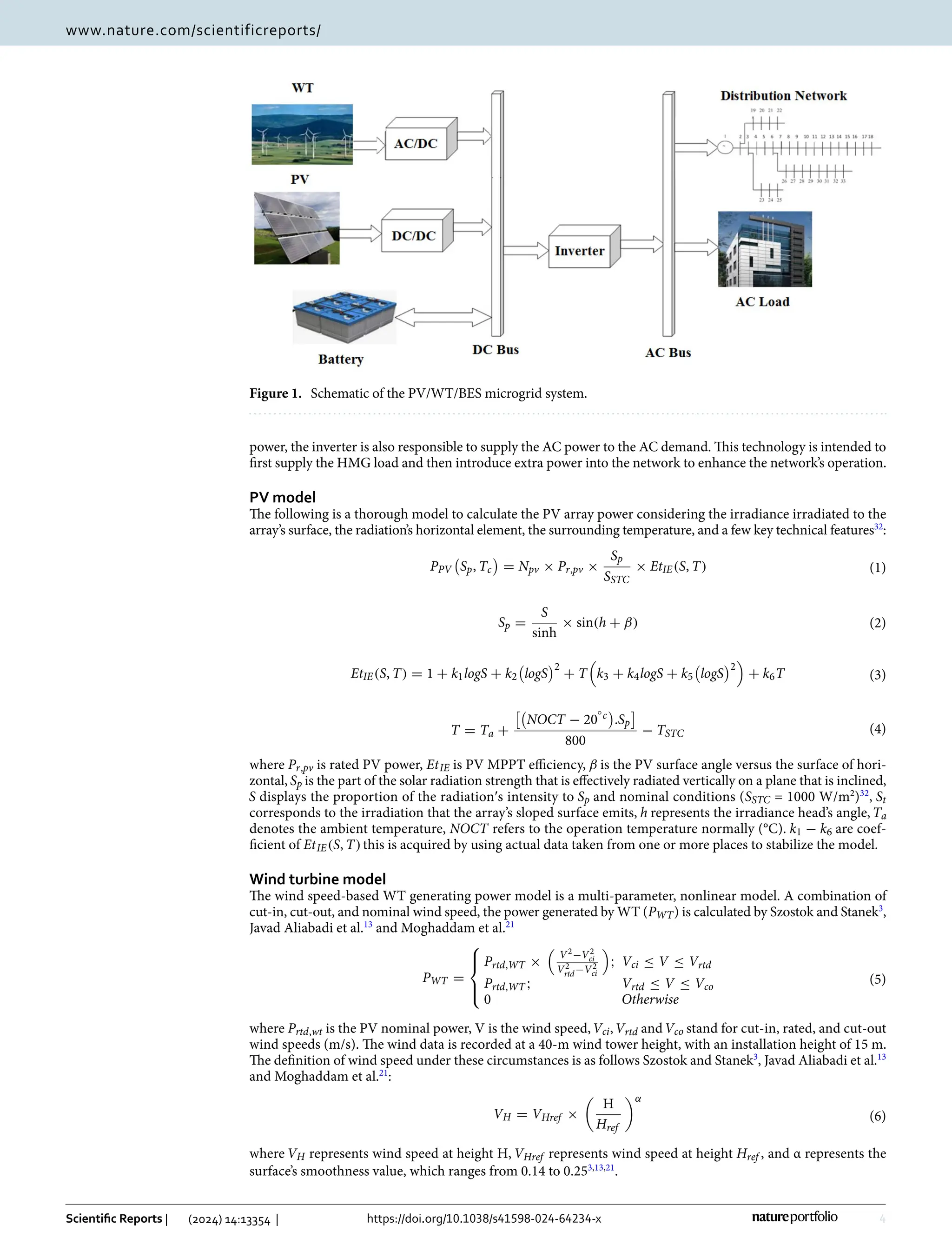
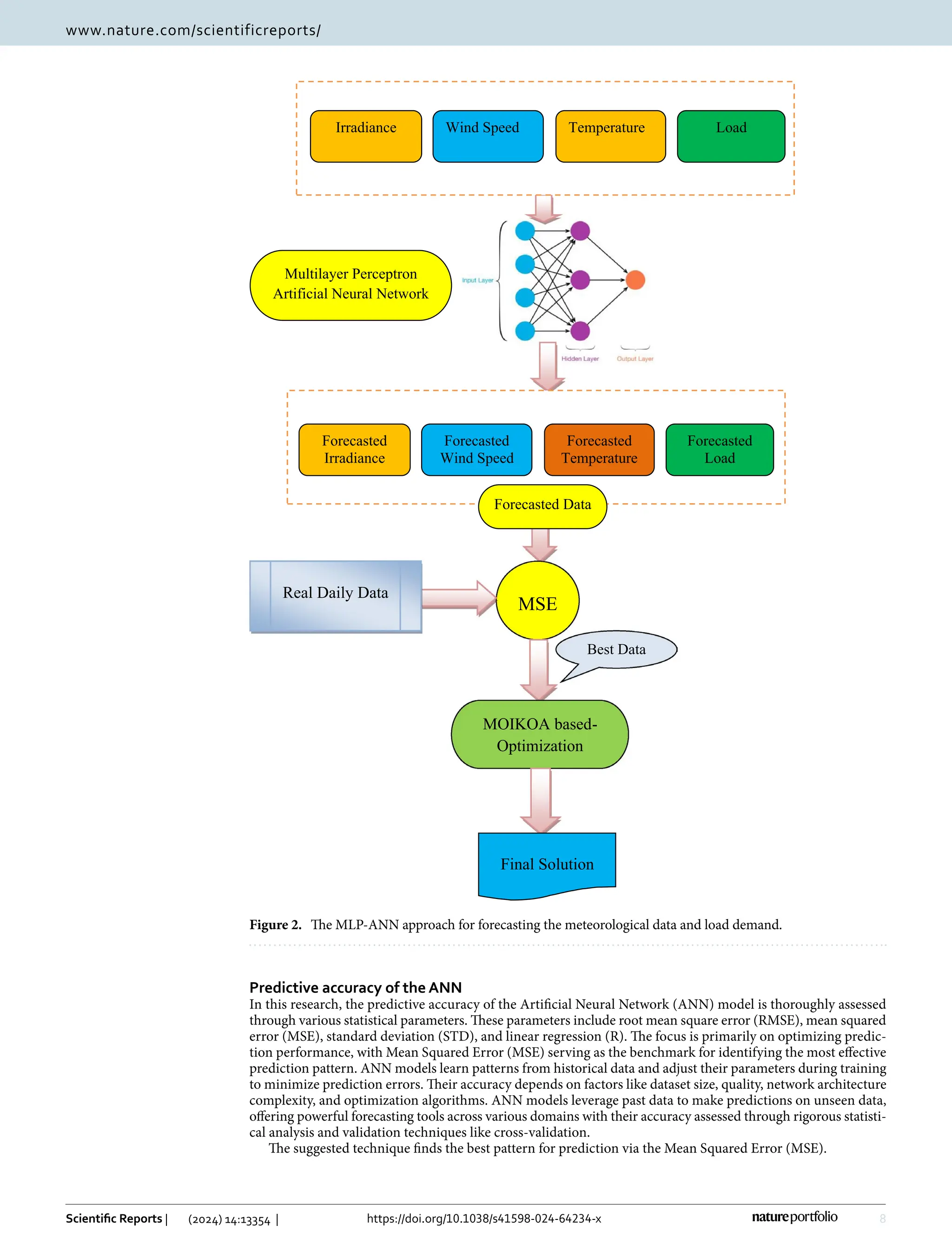
According to recent studies Nguyen et al.36
, the MLP-ANN is implemented for the prediction of time series
data as it generates more satisfactory results. To analyze temporal information effectively, MLP-ANN requires a
certain amount of memory. In ANN, memory is implemented through the use of time delays, and several different
approaches have been devised to do this. In reality, these lags are employed to fine-tune ANN’s learning process
parameters. The layers that are input, hidden, and output are the three layers that make up this framework.
Figure 2 shows single variation inputs, denoted as i(n-1),i(n-2)…i(n−p) match samples of earlier data, where
O(n) represents the forecast’s outcome value, while p indicates the prediction order.
Proposed optimizer
Overview of the Kepler optimization algorithm (KOA)
The KOA inspiration
Kepler’s principles of planet motion are its main source of motivation. Kepler’s laws state that the Earth’s orbital
acceleration, gravitational force and mass, and position of the planet are the four operators that influence a
planet’s course around the Sun. The mathematical framework of the suggested KOA was created using the opera-
tors. Because the planets in the KOA are in different conditions around the Sun at various times, the search space
is more effectively investigated and utilized. Like other population-centered metaheuristic methods, KOA begins
the search with an assortment of starting objects (the applicant solutions) that have probabilistic orbitals. At this
point, each object’s orbital location is initialized to be random. KOA evaluates the fitness of the initial set and
repeats until the termination requirement is met. Since the word time is frequently applied in solar
systems39
and cosmology, it is employed in place of iteration in the present investigation.
The KOA steps
The process of initializing process, defining the effect of gravity, computing an object’s velocity, departing from
the ideal location, updating objects’ locations, maintaining distance from the sun, and exclusivity are some of
the KOA stages that are covered in this part.
Step 1 (the procedure under the initialization): The formula listed
below31
will be used in this procedure to
randomly disperse planets are N, also known as the population size, in d-dimensions, which indicate the choice
variables:
where X
j
i,up and X
j
i,low denote the highest and lowest boundaries, correspondingly, of the
jth
choice variable, and
rand[0,1] is an amount produced at random ranging from 0 to 1. Additionally, Xi shows the
ith
planet.
McDermott31
initializes the orbital eccentricity (e) for each ith object.
where an arbitrary number created inside the interval [0, 1] is denoted by rand[0,1]. Lastly,
McDermott31
initial-
izes the orbital time (T) for each and every ith object.
where r is a random number that is produced using the typical distribution as the starting point.
Step 2 (Determining the force of gravitational (F)): The Sun is the central component of the radiation structure
because it is the biggest item within the system and uses its gravity to direct the motion of the other objects. A
planet’s speed is determined by the Sun’s gravitational pull. A planet’s speed of orbit increases with increasing
solar proximity, and vice versa. The universal rule of gravity, defined as follows, provides the Sun’s gravitational
attraction XS and each planet Xi
31
where Ms and mi are the normalized results of MS and mi, which stand for the mass of of XS and Xi, µ is universal
gravitational unchanged,
ei is the eccentricities of a planet’s the orbit of the earth, which ranges from 0 to 1,
r1 is
(27)
R =
N
p=1 (Yp − Xp)2
N
p=1 (Xp − Yave)2
(28)
MSE =
1
N
N
p=1
(Yp − Xp)2
(29)
RMSE =
1
N
N
p=1
(Yp − Xp)2
(30)
X
j
i = X
j
i,low + rand[0,1] ×
X
j
i,up − X
j
i,low
,
i = 1, 2, . . . , N.
j = 1, 2, . . . , d.
(31)
ei = rand[0,1], i = 1,2, . . . , N.
(32)
Ti=|r|, i = 1,2, . . . , N.
(33)
Fgi(t) = ei × µ(t) ×
Ms × mi
R
2
i + ε
+ r1](https://image.slidesharecdn.com/s41598-024-64234-x-240928215213-e48b7496/75/Optimization-of-Photovoltaic-wind-battery-energy-based-microgrid-9-2048.jpg)
![11
Vol.:(0123456789)
Scientific Reports | (2024) 14:13354 | https://doi.org/10.1038/s41598-024-64234-x
www.nature.com/scientificreports/
where r3 and
r4 are arbitrarily produced numerical numbers at range [0, 1], −
→
r 5 and −
→
r 6 are a couple of vectors
containing arbitrary numbers from 0 to 1, Vi(t) denotes the acceleration of object i, and
−
→
X i indicates object i.
−
→
X a and
−
→
X b are randomly chosen solutions taken from the population,
MS and mi denote XS and Xi’s respective
masses; µ(t)is constant of the universal
gravitational31
. ɛ is a tiny quantity that eliminates a division by zero error.
where Ti stands for object i’s orbital period.
Ri−norm(t)is Euclidian normal distance among XS and Xi, and it is determined by
If Ri−norm(t) ≤ 0.5, the object is near the Sun and will accelerate to avoid falling in its direction due to the
powerful attraction of the Sun.
Step 4 (Leaving the local optimal): Most objects in the radiation system’s axes of rotation in a counterclock-
wise direction around the Sun, but some objects also rotate in a circular motion direction. This characteristic
is exploited by the recommended method to escape local optimum areas. By considering a flag F to alter the
search orientation and increase the likelihood of agents successfully exploring the search space, the suggested
KOA mimics this pattern of action.
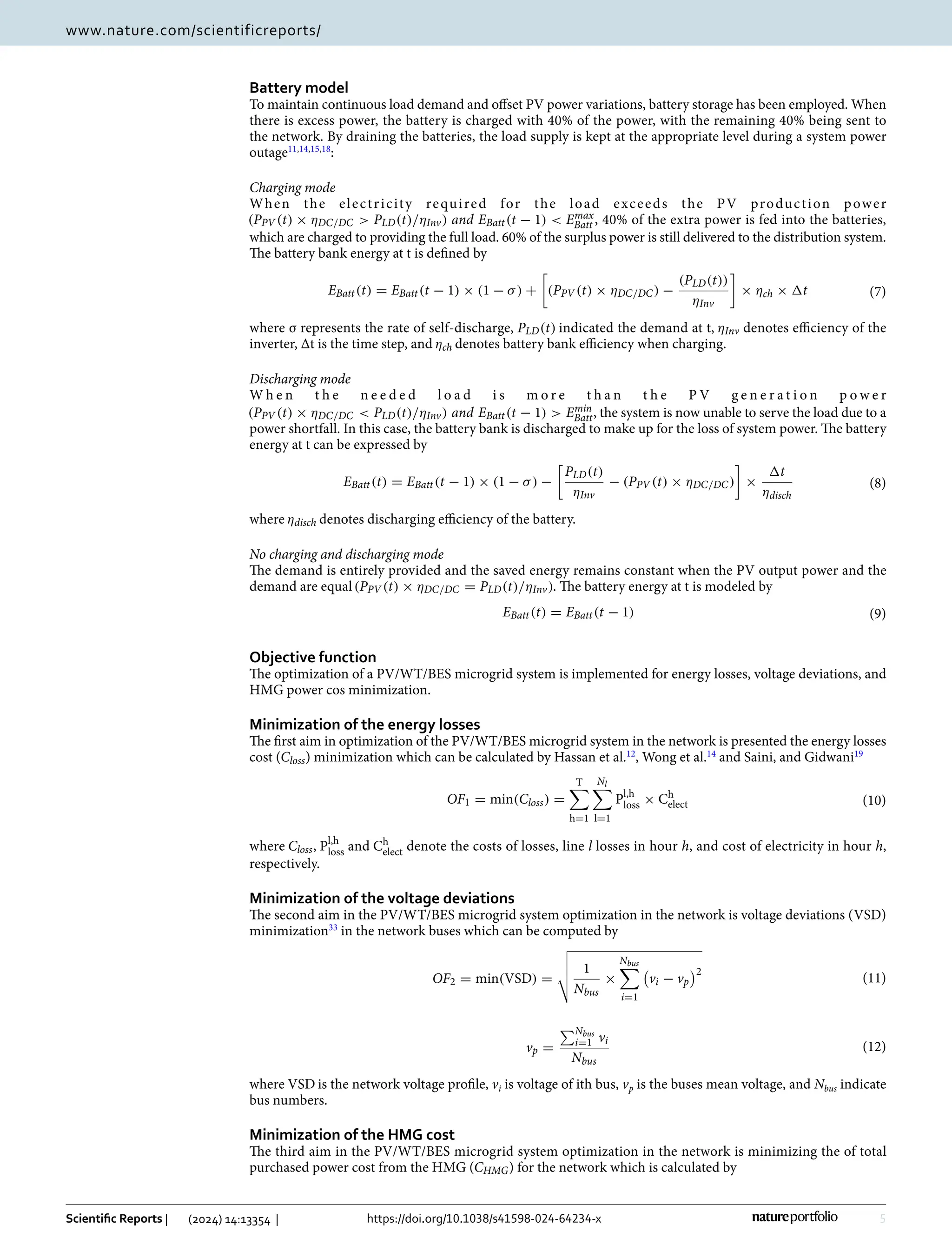
Step 5 (Updating objects’ positions): Objects rotate in a direction that brings them closer to the Sun for a while
before turning aside. The two main stages of the suggested algorithm—the discovery and utilization phases—
simulate this tendency. KOA looks for new locations near the best options when utilizing solutions closer to
the Sun to identify new items to explore and discover new solutions. The areas of exploration and harvesting
surrounding the Sun are depicted in Fig. 3. The objects’ distance from the Sun during the exploration stage sug-
gests that the recommended technique more effectively covers the whole search region. Following the preceding
procedures, McDermott31
updates the position of every object that is far from the Sun.
where
−
→
X i(t + 1)is the most favorable location of the Sun found to date,
−
→
V i(t)denotes the object i new position
at time t+1, XS(t)is the speed of object i required for reaching the new position, and ℑ is employed as a flag to
modify the orientation of the search.
Step 6 (Updating distance with the Sun): KOA prioritizes exploitation actor optimization while planets are
close to the Sun and optimize the exploration operator when planets are far from the Sun. The regulatory param-
eter h’s value, which varies steadily with time, determines the application of these principles. If this quantity is
modest, to exploit, the exploitation operator is employed for the areas surrounding the best-so-far answer if the
distance between the Sun and planets is short. On the other hand, when this is great, an exploring operator is
used to increase the planet’s orbital dispersion from the Sun. As stated in Algorithm 1, this idea is randomly
swapped out to enhance KOA’s research and extraction operators even further. The following is a description of
this principle’s
model31
:
As explained following
McDermott31
, ℎ denotes an adaptive factor that controls the separation across the
Sun and the present-day planet.
(49)
U2 =
0r3 ≤ r4
1 Else
(50)
ai(t) = r3 ×
T2
i ×
µ(t) × (MS + mi)
4π2
1/3
(51)
Ri−norm(t) =
Ri(t) − min(R(t))
max(R(t)) − min(R(t))
(52)
−
→
X i(t + 1) =
−
→
X i(t) + F ×
−
→
V i(t) + (Fgi
+ |r|) ×
−
→
U × (
−
→
X S(t) −
−
→
X i(t))
(53)
−
→
X i(t + 1) =
−
→
X i(t) ×
−
→
U 1 +
1 −
−
→
U 1
× (
−
→
X i(t) +
−
→
X S +
−
→
X a(t)
3
+ h × (
−
→
X i(t) +
−
→
X S +
−
→
X a(t)
3
−
−
→
X b(t)))
(54)
h =
1
eηr
Figure 3.
Locations for discovery and exploitation in the area of
searches31
.](https://image.slidesharecdn.com/s41598-024-64234-x-240928215213-e48b7496/75/Optimization-of-Photovoltaic-wind-battery-energy-based-microgrid-11-2048.jpg)
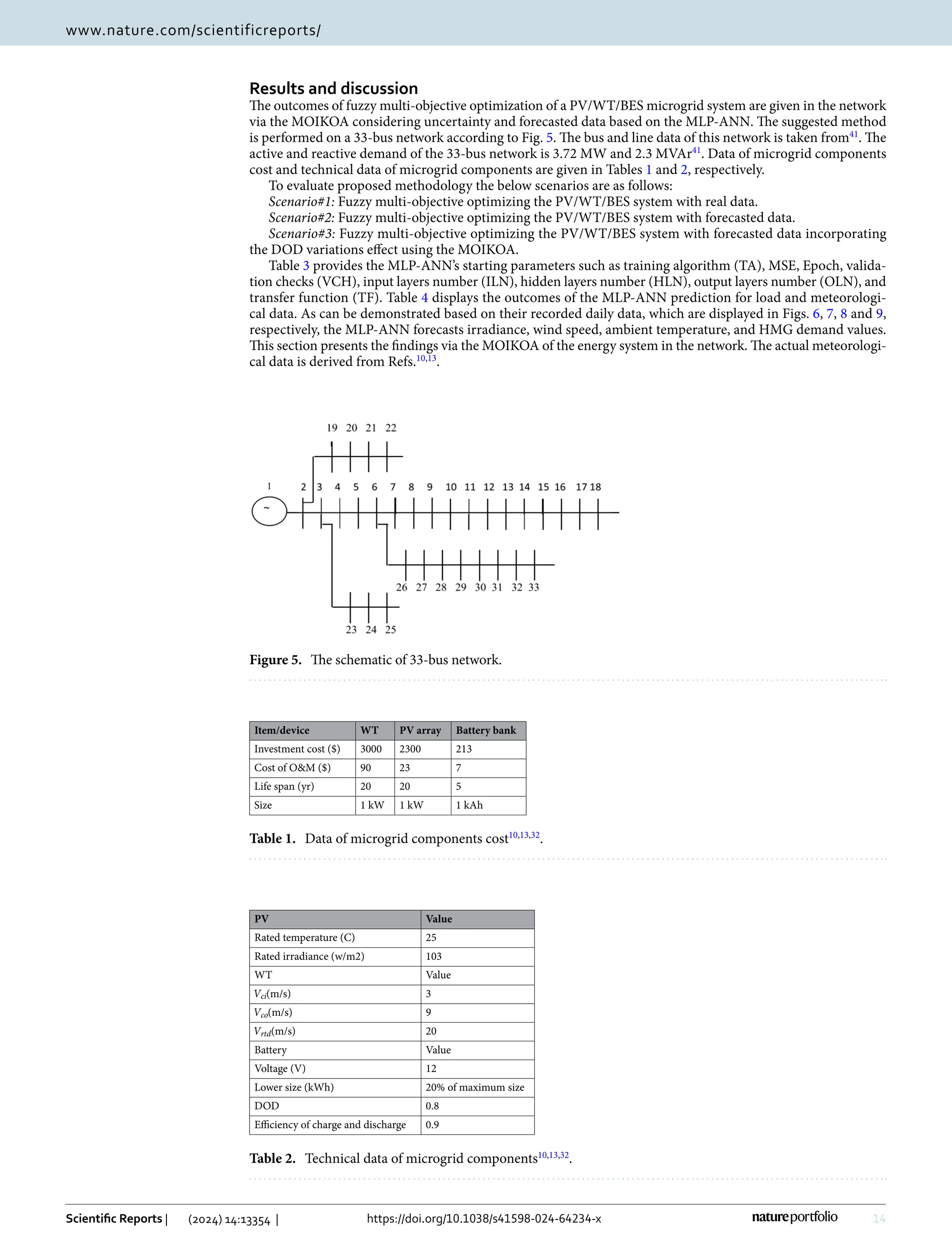
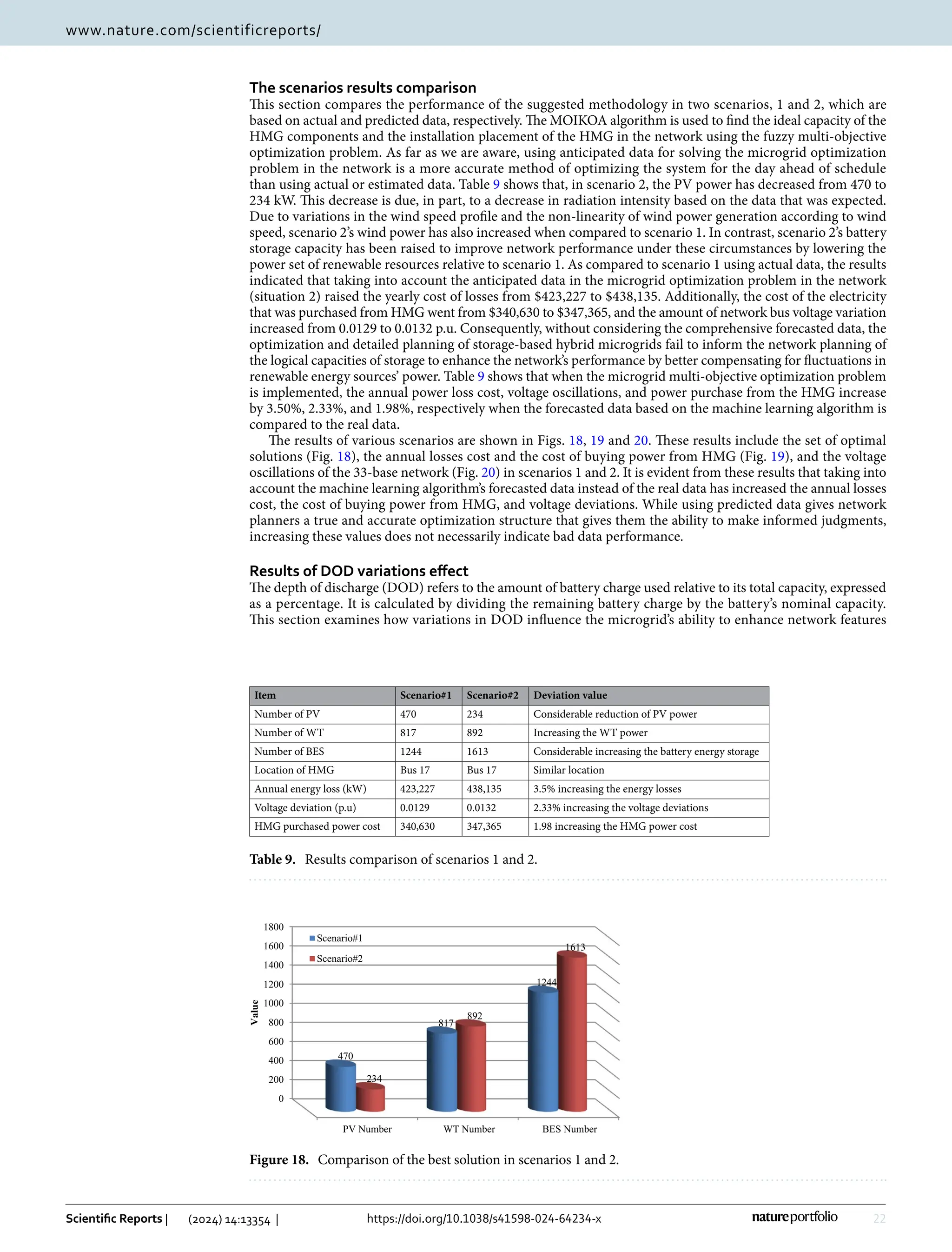
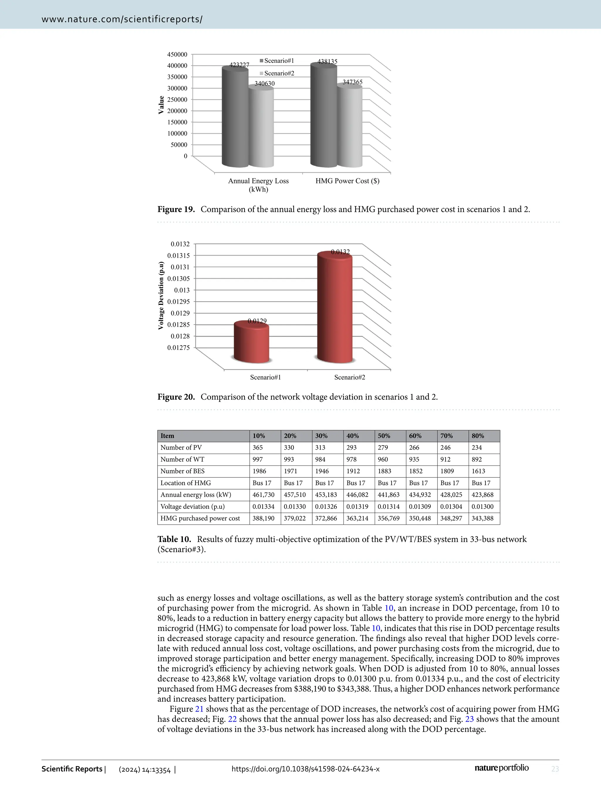
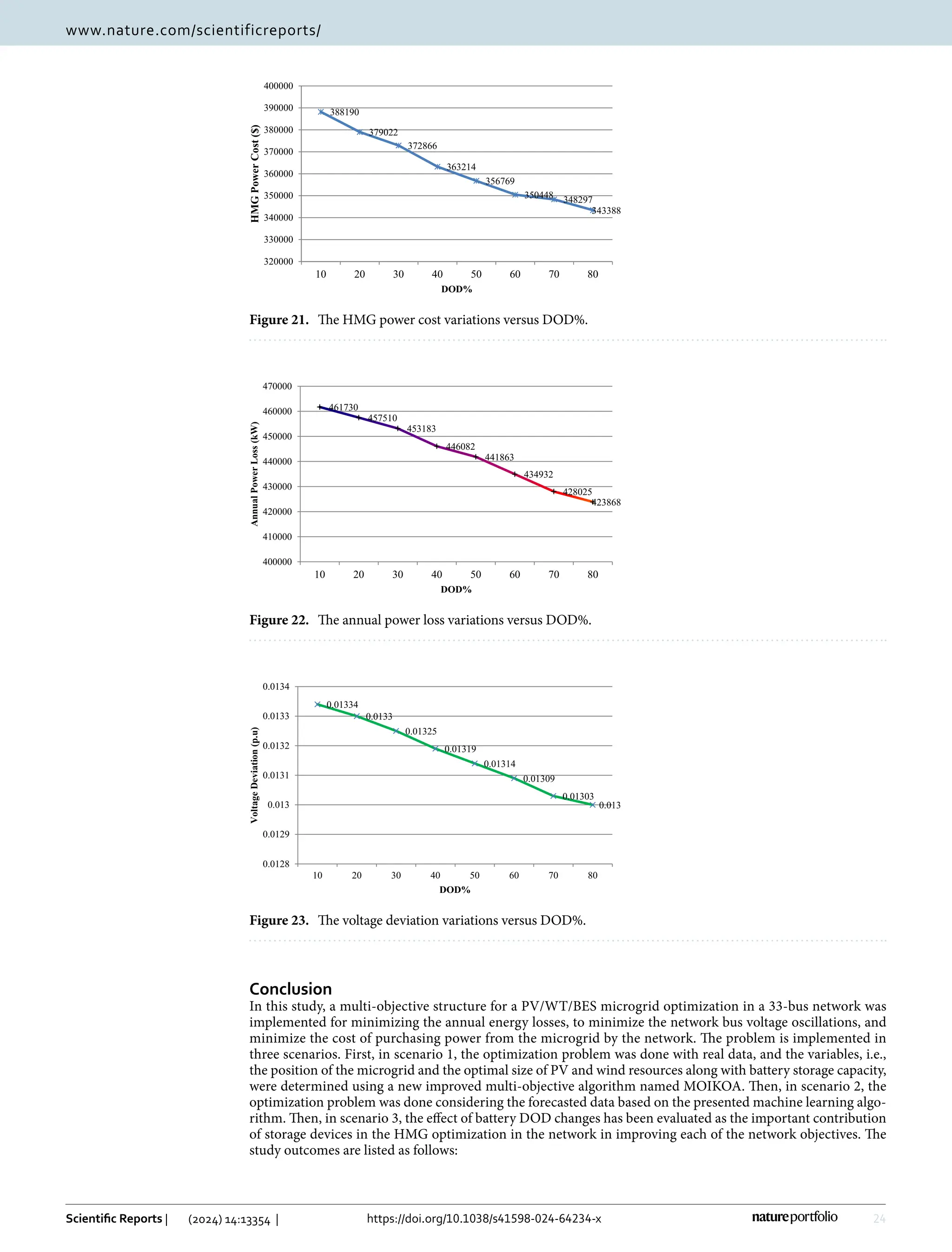


This study presents a fuzzy multi-objective optimization framework for a hybrid microgrid comprising photovoltaic, wind energy sources, and battery storage in a distribution network, utilizing a multi-objective improved Kepler optimization algorithm (MOIKOA). It employs machine learning via a multilayer perceptron artificial neural network (MLP-ANN) to forecast key meteorological and load data, demonstrating significant benefits over traditional optimization methods in minimizing energy losses, voltage oscillations, and costs associated with energy purchase. Results indicate that optimizing with forecast data and investigating the battery's depth of discharge can enhance microgrid performance, highlighting areas previously underexplored in existing literature.