Operations-Management.pdf

Operations Management
B. Mahadevan
Indian Institute of Management Bangalore
JSNR_DreamTech Pearson_Operations Management_Text.pdf 1 5/3/2019 11:59:54 AM

Chief Academic Officer
Dr. Arun Mohan Sherry
M. Sc. (Gold Medalist), M. Tech (Computer Science - IIT Kharagpur), Ph. D.
NMIMS Global Access—School for Continuing Education
Reviewed By
KaliCharan Sabat
NMIMS Global Access—School for Continuing Education
NMIMS Global Access - School for Continuing Education
V. L. Mehta Road, Vile Parle (W), Mumbai – 400 056, India.

Copyright © 2019 Pearson India Education Services Pvt. Ltd
This book is sold subject to the condition that it shall not, by way of trade or otherwise, be lent,
resold, hired out, or otherwise circulated without the publisher’s prior written consent in any
form of binding or cover other than that in which it is published and without a similar condition
including this condition being imposed on the subsequent purchaser and without limiting the
rights under copyright reserved above, no part of this publication may be reproduced, stored in
or introduced into a retrieval system, or transmitted in any form or by any means (electronic,
mechanical, photocopying, recording or otherwise), without the prior written permission of both
the copyright owner and the publisher of this book.
ISBN 978-93-530-6712-0
First Impression
Published by Pearson India Education Services Pvt. Ltd, CIN: U72200TN2005PTC057128.
Head Office: 15th Floor,Tower-B,World Trade Tower, Plot No. 1, Block-C, Sector-16,
Noida 201 301, Uttar Pradesh, India.
Registered Office: 4th Floor, Software Block, Elnet Software City,TS-140, Block 2 & 9,
Rajiv Gandhi Salai,Taramani, Chennai 600 113,Tamil Nadu, India.
Fax: 080-30461003, Phone: 080-30461060
Website: in.pearson.com, Email: companysecretary.india@pearson.com
Printed in India by Repro India Ltd., Surat.

1. Operations Management Trends and Issues: Introduction to Operations Management, Manufacturing and
Service Sector Trends in India, Service operations management, Operations Management Functions, Challenges in
2. Facilities Location: Factors Affecting Location Decisions, Location Planning Methods- Centre of gravity Method,
Load–Distance Method, Transportation methods, Globalization of Operations
3. Plant Layout: The Process–Product Matrix, Layout Planning, Types of Layouts- Process Layout, Product Layout,
Group Technology Layout, Fixed Position Layout, Performance measures for Layout Design, Design of Process
Layouts, Design of Product Layouts, Design of Group Technology Layouts, Technology issues in Process Design
4. Productivity and Production: Aggregate Operations Planning, Strategies for Aggregate Operations Planning- Level
Strategy, Chase Strategy, and Mixed Strategy, Master Operations Scheduling
5. Manufacturing Economics: Dependent Demand Attributes, MRP System, Capacity Requirements Planning,
Manufacturing Resources Planning (MRP II), Enterprise Resource Planning (ERP), Resources Planning in Services
6. Inventory Management and Models: Inventory Planning for Independent Demand Items, Types of Inventory,
Inventory Costs, Inventory Control Systems, Inventory Classification Schemes, Inventory Planning for Single-Period
Demand
7. TotalQualityManagement:QualityGurus,DefinitionsofQuality,TotalQualityManagement,QualityManagement
Tools, Quality Certifications and Awards
8. Theory of Constraints: The Need for Scheduling, Scheduling of Flow Shops, Scheduling of Job Shops, Operations
Planning and Control Based on the Theory of Constraints
C U R R I C U L U M

1 Operations Management: Trends and
Issues 2
IDEAS AT WORK 1.1: NARAYANA HEALTH (NH): A
JOURNEY THAT BEGAN WITH WINING THE HEART OF
INDIA 3
1.1 Introduction to Operations
Management 4
1.2 Manufacturing and Service Sector Trends
in India 5
1.3 Services as a Part of Operations
Management 6
Intangibility 7
Heterogeneity 7
Simultaneous Production and Consumption 8
VIDEO INSIGHTS 1.1 8
Perishability 8
IDEAS AT WORK 1.2: OPERATIONS MANAGEMENT
IN SERVICE SYSTEMS 8
1.4 Operations as a Key Functional Area 10
1.5 Operations Management: A Systems
Perspective 12
1.6 Operations Management Functions 14
Design Versus Operational
Control Issues 14
Long-term Versus Short-term Issues 15
1.7 Challenges in Operations
Management 15
Competitive Pressure due to Economic
Reforms 16
Growing Customer Expectations 16
Technological Developments 17
Environmental Issues 17
1.8 Current Priorities for Operations
Management 18
IDEAS AT WORK 1.3: INDIA – AN EMERGING
GLOBAL MANUFACTURING BASE 19
Summary 19
Review Questions 20
Net-Wise Exercises 20
Multiple-choice Questions 21
2 Facilities Location 22
IDEAS AT WORK 2.1: AKSHAYA PATRA: THE
NATION-WIDE MID-DAY MEAL SCHEME OF
ISKCON 23
2.1 Globalization of Operations 24
Regulatory Issues 24
Factor Advantages 25
Expanding Markets in Developing Countries 25
2.2 Factors Affecting Location Decisions 27
Market-related Issues 27
IDEAS AT WORK 2.2: ARAVIND EYE HOSPITAL’S
APPROACH TO LOCATION OF HEALTHCARE
DELIVERY SYSTEMS 28
Cost-related Issues 29
Regulatory and Policy Issues 29
Other Issues 29
2.3 Location Planning Methods 29
Location Factor Rating 29
IDEAS AT WORK 2.3: SPECIAL ECONOMIC ZONES: A
POLICY ANGLE TO LOCATION PLANNING 30
The Centre-of-gravity Method 32
The Load–Distance Method 34
The Transportation Model 35
2.4 Other Issues in Location
Planning 38
Summary 39
Formula Review Questions 40
Review Questions 40
Problems 40
Mini Project 42
Case Study 43
3 Plant Layout 50
IDEAS AT WORK 9.1: PROCESS DESIGN AT MILLTEC
MACHINERY 51
3.1 Determinants of Process Characteristics
in Operations 52
Volume 52
Variety 52
Flow 52
C O N T E N T S

viii Contents
3.2 Types of Processes and Operations
Systems 53
Continuous Flow Systems 53
IDEAS AT WORK 9.2: THE POLYESTER FILAMENT
YARN PLANT AT RELIANCE INDUSTRIES
LIMITED 56
Intermittent Flow 57
Jumbled Flow Systems 59
IDEAS AT WORK 9.3: PROCESS REDESIGN FOR
IMPROVING FLOW 59
3.3 The Process–Product Matrix 61
3.4 Layout Planning 62
3.5 Types of Layouts 63
Process Layout 63
Product Layout 64
Group Technology Layout 66
Fixed Position Layout 66
IDEAS AT WORK 9.4: WORKPLACE ORGANIZATION
AT THERMAX 67
3.6 Performance Measures for Layout
Design 68
3.7 Design of Process Layouts 69
The Qualitative Approach to Layout Design 70
The Quantitative Approach to Layout
Design 71
Software Packages for Layout Design 71
3.8 Design of Product Layouts 72
3.9 Design of Group Technology
Layouts 75
3.10 One Worker–Multiple Machine Layouts 77
3.11 Technology issues in Process Design 78
Flexible Manufacturing Systems 78
Automated Material-handling Systems 80
3.12 Complexity in Operations
Management 81
Summary 82
Formula Review 82
Review Questions 82
Problems 83
Mini Project 84
Case Study 85
4 Productivity and Production 90
IDEAS AT WORK 15.1: OPERATIONS
PLANNING AT AMAZON TO IMPROVE SERVICE
EFFECTIVENESS 91
4.1 Planning Hierarchies in
Operations 92
4.2 Aggregate Operations Planning 93
4.3 The Need for Aggregate Operations
Planning 94
4.4 Alternatives for Managing Demand 96
Reservation of Capacity 96
Inﬂuencing Demand 96
4.5 Alternatives for Managing Supply 96
Inventory-based Alternatives 97
Capacity Adjustment Alternatives 97
4.6 Basic Strategies for Aggregate
Operations Planning 99
Level Strategy 99
Chase Strategy 100
Mixed Strategy 101
4.7 Aggregate Operations Planning
Methods 112
Heuristic Methods for AOP 112
Optimal Methods for AOP 113
4.8 Operations Research Tools for Operations
Planning 113
Aggregate Operations Planning Using the
Transportation Model 113
IDEAS AT WORK 15.2: USE OF SPREADSHEETS FOR
AGGREGATE PRODUCTION PLANNING 114
The Linear Programming Model for AOP 116
The Linear Decision Rule (LDR) 119
4.9 Master Operations Scheduling 119
Summary 122
Review Questions 122
Problems 123
Case Study 125

Contents ix
5 Manufacturing Economics 128
IDEAS AT WORK 16.1: ERP IMPLEMENTATION AT
HPCL 129
5.1 Dependent Demand Attributes 130
5.2 Planning A Framework: The Basic
Building Blocks 131
Multiple Levels in Products 131
Product Structure 133
The Bill of Materials (BOM) 135
Time Phasing the Requirement 137
Determining the Lot Size 139
Incorporating Lead-time Information 141
Establishing the Planning Premises 142
5.3 MRP Logic 144
5.4 Using The MRP System 148
Updating MRP Schedules 148
Safety Stock and Safety Lead Time 149
5.5 Capacity Requirements Planning
(CRP) 151
5.6 Distribution Requirement Planning
(DRP) 151
5.7 Manufacturing Resources Planning
(MRP II) 153
IDEAS AT WORK 16.2: OPEN SOURCE ERP
SOLUTION FOR VENKATESWARA HATCHERIES 154
5.8 Enterprise Resource Planning (ERP) 154
5.9 Resources Planning in Services 156
IDEAS AT WORK 16.3: SERVICES RESOURCES
PLANNING (SRP): AN ERP SOLUTION FROM
RAMCO 156
Summary 157
Problems 158
Mini Projects 161
6 Inventory Management
and Models 164
IDEAS AT WORK 17.1: INVENTORY MANAGEMENT
IN A CONSUMER PRODUCTS COMPANY 165
6.1 Inventory Planning for Independent
Demand Items 166
Continuous Demand 166
Uncertainty of Demand 166
6.2 Types of Inventory 167
Seasonal Inventory 167
Decoupling Inventory 167
Cyclic Inventory 168
Pipeline Inventory 168
Safety Stock 168
6.3 Inventory Costs 169
Inventory-carrying Cost 169
Cost of Ordering 170
Cost of Shortages 171
6.4 Inventory Control for Deterministic
Demand Items 171
Problems in the EOQ model 173
6.5 Handling Uncertainty in Demand 174
6.6 Inventory Control Systems 176
The Continuous Review (Q) System 176
The Periodic Review (P) System 177
Issues in the P and Q Systems of Inventory
Control 178
6.7 Selective Control of Inventory 180
ABC Classiﬁcation 180
Other Classiﬁcation Schemes for Selective
Control 182
IDEAS AT WORK 17.2: THE INVENTORY
CONTROL SYSTEM OF A PETROCHEMICAL
MANUFACTURER 183
6.8 Inventory Planning for Single-Period
Demand 183
6.9 Other Issues in Inventory Planning and
Control 184
Summary 185
Formula Review 185
Problems 186
Mini Projects 189
Case Study 189
7 Total Quality Management 196
IDEAS AT WORK 12.1: POKA YOKE FOR DEFECT
PREVENTION 197
7.1 The Quality Revolution 198
7.2 Quality Gurus 198
William Edwards Deming 198
Joseph M. Juran 199

x Contents
Philip B. Crosby 199
Karou Ishikawa 199
Shigeo Shingo 200
Genichi Taguchi 200
7.3 Definitions of Quality 201
Conformance to Specifications 201
Fulfilling Customer Needs 201
Fitness for Use 201
7.4 Total Quality Management 202
Commitment of Top Management 203
IDEAS AT WORK 12.2: QUALITY POLICY IN SOME
ORGANIZATIONS 203
Employee Involvement 204
Addressing Training Requirements 205
7.5 Quality Management Tools 205
Histograms 207
Pareto Diagrams 207
Cause and Effect (Fishbone) Diagrams 207
CEDAC 208
Poka Yoke 209
IDEAS AT WORK 12.3: MATRIX DIAGRAM FOR
ENHANCING THE COMPETITIVENESS OF A
PRODUCT 210
Quality Function Deployment 211
Quality Costing 212
7.6 Quality Certifications
and Awards 213
Quality Awards 213
Quality Certifications 214
IDEAS AT WORK 12.4: SRF’S TQM JOURNEY
TOWARDS THE DEMING PRIZE 216
7.7 Design of Quality Assurance
Systems 218
Summary 219
Problems 220
Mini Projects 221
Case Study 222
8 Theory of Constraints 226
IDEAS AT WORK 18.1: SCHEDULING THE ORDER
PROCESSING OPERATION AT BLOCKBUSTER
DISTRIBUTION CENTER 227
8.1 The Need for Scheduling 228
8.2 Scheduling: Alternative Terms 229
Planning-related Terms 229
Technological Constraints-related
Terms 229
Administration-related Terms 230
8.3 The Loading of Machines 230
8.4 The Scheduling Context 231
IDEAS AT WORK 18.2: SCHEDULING OF PHYSICIAN
IN THE EMERGENCY DEPARTMENT OF A
HOSPITAL 233
Scheduling Rules 234
Performance Criteria 235
8.5 Scheduling of Flow Shops 237
Johnson’s Rule 238
8.6 Scheduling of Job Shops 240
8.7 Input–Output Control 242
8.8 Operational Control Issues in Mass
Production Systems 242
Machine Redeployment 244
Altering Operator Allocations 244
Adjusting Material Feed Rates 244
8.9 Operations Planning and Control Based
on the Theory of Constraints 244
Measures of Performance 244
The Analogy of Marching Soldiers 245
Synchronous Manufacturing 246
Constraints in a Manufacturing System 247
The Drum–Buffer–Rope (DBR)
Methodology 248
Summary 249
Formula Review 249
Problems 250
Mini Projects 252

2
C H A P T E R
CRITICAL
QUESTIONS
Operations Management:
Trends and Issues 1
After going through this chapter, you will be able to answer the following questions:
• What do you understand by the term operations management?
• What is the status of the manufacturing and service industries in India?
• What are the emerging opportunities and challenges for operations management?
• Can the principles of operations management be applied to both manufacturing and
service organizations?
• What is the role of operations in an organization?
• What are the key components of an operations management system? What is the nature
of the interaction among them?
The success of Narayana Health
(NH) is mainly due to the proper
implementation of operations
management in its day-to-day activities.
The growth of NH to 14 multi-speciality
hospitals is mainly because of its
planning, passion, and compassion;
this is what operations management
is all about. Managing a workforce of
12,000 is mainly attributed mainly to
strategic thinking and implementation.
The success rate is made possible by
employing cost reduction in several
methods. The main vision of the NH
group is not to lose a single patient in
terms of want of money and conducting
the surgeries in a cost-effective manner.
Source: Franck Boston. Shutterstock

Operations Management: Trends and Issues 3
Narayana Health (NH): A Journey That Began with Wining the Heart of India
Indians are three times prone to heart diseases
than Europeans. By 2013, while there is a need
for 2.5 million heart surgeries per year in India, we are
doing only 90,000. Moreover, India produces 80 cardi-
ologists a year compared to 800 in the US. There is a huge
shortage of doctors and paramedical staff in the country.
To complicate the matter even more, 70% doctors are in
urban areas, whereas 70% people live in rural areas. This
appears to be a serious problem of lack of adequate health-
care for the citizens. However, a closer look at the story of
Narayana Health (NH) suggests that mass healthcare cover
is not about money but about planning, passion, and com-
passion. Operations Management can work at its best to
address such problems.
NH journey first started with a 300-bed hospital
started by Dr. Devi Shetty in the outskirts of Bangalore
city in 2001 that began providing heart surgeries to
patients at significantly low costs. Currently, the group
has 14 hospitals in multiple locations with multiple spe-
cialties that offer a total of 5,700 beds. Over the next 18
months, there are plans to add new hospitals in Siliguri,
Bhubaneswar, Mysore, Mumbai, and Delhi in addition
to Cayman Islands and Malaysia, which will add another
2,500 beds capacity to the NH network. There are plans
to expand this to about 30,000 beds by 2020. On account
of this, the work force is likely to grow from the current
strength of 12,000 to nearly 40,000. Managing such a
massive expansion requires sound strategic thinking,
creation of new facilities in a cost-effective manner, and
operating them on a day-to-day basis with better plan-
ning. All these issues belong to the domain of Opera-
tions Management.
Many of the operational aspects of the NH network
are governed by the vision that nobody should go back
from the hospital for want of money. A heart surgery
package at NH could be anywhere between `75,000
and `150,000 compared to a typical cost of `300,000
in other hospitals. Achieving such dramatic cost reduc-
tion calls for employing several methods. These include
input cost reduction, benefiting from process innova-
tions and scale economies, and bringing innovative
ideas in design of facilities and resource deployment.
Further, productivity improvements would be very cru-
cial and an ongoing activity in such a system. In NH, we
find several examples illustrating these.
Due to volumes and supplier development
efforts, NH is able to buy a pair of glove at `4.50 as
against `9.50 by directly sourcing it from Malaysia.
Many of the expensive equipment such as MRI scan
machine are installed by vendors on a pay-per-use
model rather than an outright purchase. This brings
down the cost of an MRI scan and also increases its
utilization. Hospitals are located on the outskirts of
the cities to bring down the capital costs. The Mysore
cardiac hospital was built using pre-fabricated materi-
als and has no air-conditioning, except in operation
theatres, thereby bringing down the cost of the facility
dramatically low.
Another strategy to bring down the cost is to
increase the volume of patient flow. To achieve this, NH
has diversified into multi-specialties (such as Eye care,
Orthopaedics, Neuroscience, and so on). Furthermore,
NH recruits the best doctors and pays them as per the
best industry standards. However, they are convinced to
work a little extra. For the doctors at NH, 10 years ago,
the plan was to do five surgeries a day with a 150-bed
capacity, which itself was felt high. However, currently
with 5,700 beds, they perform 30 surgeries a day. As a
result, nearly 10–12% of all cardiac surgeries performed
in India is done in NH network.
Narayana Health is an example of a service system.
Like NH, every other service organizations as well as
manufacturing organizations face similar set of issues,
although in varying degrees. As illustrated in the case
of NH, these issues can be addressed by applying several
tools and techniques, collectively known as Operations
Management.
Source: Based on Babu, V. (2012), “Pulse on the future”, Business
World, March 5, 2012, pp 40–45; Chaki, D. (2013), “Straight from
the heart”, Business India, Sep. 30–Oct. 13, 2013, pp 61–63.
ideas
at Work
1.1
Notes

4 Chapter 1
1.1 INTRODUCTION TO OPERATIONS MANAGEMENT
Manufacturing, service, and agriculture are the major economic activities in any country. In
India, manufacturing and services together constitute nearly 75 per cent of the gross domestic
product (GDP). In recent years, growth in the GDP has been primarily due to the growth in these
sectors of the economy. Moreover, the share of the service sector in the GDP has grown steadily
from about 40 per cent to over 51 per cent between 1996 and 2006. In view of their contribu-
tion to the country’s GDP, management of manufacturing and service operations are important
economic activities. Significant improvements in productivity and cost savings can be achieved
through operations management—a discipline that focuses on activities that relate to the plan-
ning and control of operations in manufacturing and service organizations. Efficient operations
management can also have a positive impact on the overall health of the economy.
Amanufacturingfirmessentiallyengagesinconvertingavarietyofinputsintoproductsthatare
useful for individuals and organizations. For example, a manufacturer of machine tools employs
severalproductionworkers,buysrawmaterialandcomponentsfromvarioussuppliers,andmanu-
factures machine tools in a factory using an extensive array of manufacturing facilities. In this case,
the factory encompasses a large number of interrelated conversion processes for the transforma-
tion of raw material into the final product, that is, the machine tool.
A service organization, on the other hand, responds to the requirements of customers and sat-
isfies their needs through a service delivery process. Service organizations leave an impression
in the minds of their customers through their service delivery. Typical examples of such organi-
zations include management consultancies, automobile garages, hotels, hospitals and banks. A
service organization may not always make use of material inputs and may not always produce
products that are used by the customer. For instance, a law firm providing legal consultancy to
its clients may not provide material inputs to the system or produce material output. Instead, the
input and output are informational and experiential in nature. However, in the case of a service
system like an automobile garage, a restaurant or a health care system, there are material inputs
and material outputs (in the form of products consumed by the customers, as in the case of a
restaurant). Despite this difference, service systems also have a conversion process that utilizes
resources and delivers useful outputs from the system.
An operations system is defined as one in which several activities are performed to transform
a set of inputs into a useful output using a transformation process. These inputs and outputs
can be tangible, in the form of raw materials and physical products, or intangible, in the form of
information and experiences. Viewed in this manner, manufacturing and service systems could
be broadly classified as operations systems. Operations management is a systematic approach
to addressing issues in the transformation process that converts inputs into useful, revenue-gen-
erating outputs. Four aspects of this definition merit closer attention:
➱ Operations management is a systematic approach. It involves understanding the nature of issues
and problems to be studied; establishing measures of performance; collecting relevant data;
using scientific tools, techniques, and solution methodologies for analysis; and developing
effective as well as efficient solutions to the problem at hand. Therefore, for successful opera-
tions management, the focus should be on developing a set of tools and techniques to analyse
the problems faced within an operations system.
➱ Operations management involves addressing various issues that an organization faces. These issues vary
markedly in terms of the time frame, the nature of the problem, and the commitment of the
required resources. Simple problems include deciding how to re-route jobs when a machine
breaks down on a shop floor, or how to handle a surge in demand in a service system. On the
other hand, decisions such as where to locate the plant, what capacity to build in the system,
and what types of products and services to offer to the customers require greater commit-
ment of resources and time. Operations management provides alternative methodologies to
address such wide-ranging issues in an organization.
➱ Transformation processes are central to operations systems. The transformation process ensures that
inputs are converted into useful outputs. Therefore, the focus of operations management is to
address the design, planning, and operational control of the transformation process.
➱ The goal of operations management is to ensure that the organization is able to keep costs to a minimum and
obtain revenue in excess of costs through careful planning and control of operations.An appropriate perfor-
mance evaluation system is required for this. Therefore, operations management also involves
the development of performance evaluation systems and methods through which the operat-
ing system can make improvements to meet targeted performance measures.
Operations management
is a systematic approach
to addressing issues in the
transformation process that
converts inputs into useful,
revenue-generating outputs.
Notes

Since manufacturing and service organizations form the operations system, it helps to under-
stand the prevalent trends and the status of manufacturing and service organizations in India
before we dwell on the various elements of operations management.
1.2 MANUFACTURING AND SERVICE SECTOR TRENDS IN INDIA
The index of industrial production (IIP) is a measure of the growth in the manufacturing sector.
The Centre for Monitoring Indian Economy (CMIE) collects data on several macroeconomic indi-
cators, including the IIP. Table 1.1 shows some of the salient aspects of the manufacturing and
service sectors of the Indian economy. It is evident from Table 1.1 that the corporate sector has
been going through tough times. There has not been much growth in sales revenue. However,
there has been a steady increase in operating expenses and compensation to the employees. This
has resulted in a situation where the profit after tax (PAT) has been progressively and signifi-
cantly shrinking in the last three years. The service sector companies have been experiencing this
more significantly than the manufacturing sector companies as evident from the table. On the
whole, this points to the importance of deploying sound operations management practices in
both manufacturing and service sectors of the Indian economy.
Over the years, there has been an increase in raw-material consumption. This perhaps
indicates that manufacturing organizations are increasingly buying components and semi-
processed items from suppliers. Furthermore, there has been a gradual increase in the cost of
material and labour, which are primary inputs in the manufacturing system. Such an increase
in the input cost is likely to put greater pressure on firms to cut down waste and improve pro-
ductivity to remain competitive in the market. Therefore, the focus areas of operations man-
agement are likely to be in the areas of better supplier management, elimination of waste from
the system, and improvement in overall productivity. Several sectors of the industry have been
focusing on some of these initiatives.
TABLE 1.1 Salient Aspects of the Corporate Sector of the Indian Economy
Index of Industrial Production 2009–10 2010–11 2011–12 2012–13
Manufacturing 4.84 8.95 3.00 1.29
Capital goods 0.99 14.75 −3.97 −6.04
Consumer goods 7.65 8.57 4.37 2.43
Intermediate goods 6.03 7.39 −0.62 1.60
Corporate sector performance
Manufacturing sector
Sales 5.0 20.7 19.3 9.3
Operating expenses 4.8 22.3 19.6 10.1
Raw materials expenses 6.9 25.1 21.5 8.3
Compensation to employees 10.9 15.0 9.1 12.7
Profit After Tax (PAT) 43.1 15.4 18.4 −4.6
No. of companies 8751 8320 5690 3978
Non-financial services sector
Sales 8.3 15.7 13.6 2.7
Operating expenses 6.1 17.7 15.3 1.3
Compensation to employees 5.3 15.0 14.3 14.1
Profit After Tax (PAT) 15.3 −28.0 −54.5 −7.7
No. of companies 6137 6125 4328 3065
All numbers in the table represent growth % over the previous year.
Data compiled from Economic Outlook of Centre for Monitoring Indian Economy (CMIE) using their time
series data available at http://
economicoutlook.cmie.com
Notes

6 Chapter 1
Globally, India is emerging as an important manufacturing base and is competing closely with
China in attracting several multinational companies to set up their manufacturing plants. Several
studies point to emerging opportunities for Indian manufacturing to grow and attain a global
presence. India has a unique advantage in the form of abundant low-cost labour and technical
manpower. The Global Manufacturing Competitiveness Index 2013 released by Deloitte rated
India at number four, next to China, Germany, and the US among 38 countries. It predicted India
to reach the second position in the next 5 years. The report suggested that India’s rich talent pool
of scientists, researchers, and engineers as well as its large, well-educated English-speaking work-
force and democratic regime would make it an attractive destination for manufacturers. Global
manufacturing executives increasingly view India as a place where they can design, develop, and
manufacture innovative products for sale in local as well as in global markets. Therefore, Indian
manufacturing firms can, on the one hand, exploit the low-cost advantage as an entry strategy
to capture global markets and, on the other develop, unique capabilities to position as an active
participant in the global value chain.
The examples discussed here underscore the need for use of operations management to remain
competitive in business and tap the emerging opportunities in the global arena. Effective opera-
tions management also requires a greater understanding of the various activities pursued under its
banner and the critical linkages between operations and other aspects of business.
1.3 SERVICES AS A PART OF OPERATIONS MANAGEMENT
The service sector encompasses a wide spectrum of activities in every country. The growth of
the service sector in India during 2002 to 2007 has been very significant. Table 1.2 provides
some details on the share of some sectors of services in the overall GDP. The central govern-
ment began taxing three services in 1994–95. This has grown steadily, and as of 2012–13, the
number of services taxed has gone up to 119. During this period, both the number of assessees
and the service tax revenue has been growing very rapidly. According to the Central Board of
Excise and Customs (CBEC), between 1994–95 and 2012–13 the tax revenue has grown from
`4.1 billion to `1.325 trillion. These figures indicate the growing importance of services in the
Indian economy and the need to apply management practices to plan and control operations
in the service sector.
Although services and manufacturing are classified as separate sectors in a macroeconomic
sense, from the perspective of operations management, this separation is artificial. In operations
management, a “pure product” and a “pure service” are just two ends of the spectrum, and not
separate entities. In reality, a vast majority of operations share a continuum of services and prod-
ucts. Therefore, most of the principles, tools and techniques of operations management apply to
both these sectors. This product–service continuum is illustrated in Figure 1.1.
TABLE 1.2 Service Sectors in India: Share of GDP in Percentage
2008–09 2009–10 2010–11 2011–12 2012–13#
Service sector growth rates in GDP
Trade, hotels, transport, and
communications
16.9 16.5 17.2 18.0 25.1
Transport, storage, and communications 7.8 7.7 7.3 7.1
Financial services, insurance, real estate,
and business services
15.9 15.8 16.0 16.6 17.2
Community, social, and personal Services 13.3 14.5 14.0 14.0 14.3
Construction 8.5 8.2 8.2 8.2 8.2
Total (including construction) 62.4 62.7 62.6 63.9 64.8
# Advanced Estimate
* Compiled from Chapter 10 on Services Sector in Economic Survey 2012–13, Government of India, Ministry
of Finance, Economic Division. For more details see http://indiabudget.nic.in
Notes

Services such as management consulting, health spas, and education have dominant service
attributes. They form one end of the spectrum. Similarly, manufacturing and supply of machine
tools, gadgets, and consumables have a dominant product attribute, and they form the other end
of the spectrum. However, several businesses share both service and product attributes. Take the
case of automobiles. There is a product attribute in it since it involves the physical structure of
the passenger car. On the other hand, there is also the experiential component of using the car,
which forms a significant part of the product. This is the service component. Similarly, in the
case of a restaurant, the food items share both product and service attributes. There are certain
important differences between services and manufacturing. Let us take a brief look at each of
these differences.
Intangibility
Fundamentally, services differ from manufacturing with respect to tangibility. Because services
are experiences rather than objects, they cannot be touched, tasted or felt as in the case of objects.
At the most, the recipients of services can form an opinion (based on some personal assessment)
about the quality of the service offered. This has important implications for defining and assess-
ing the quality of the service.
On the other hand, in a product-oriented operation, the product is defined by certain attrib-
utes and the customer faces less ambiguity with respect to the product, its attributes, and its
performance. This is because the customer can touch and feel the product and make his/her own
assessment of the product.
Heterogeneity
The second differentiating aspect of services is the high degree of heterogeneity associated with
them. Since the experiential component is dominant in a service, it is likely that no two services
are exactly alike. The differences are attributed to the differences in the service receivers (cus-
tomers), the service providers, and other parameters of the service delivery system. Therefore,
a dentist attending to two consecutive patients having identical ailments may provide more or
less the same type of service. Nevertheless, the two patients may have different perceptions of
the quality of the service and may have different satisfaction levels. Moreover, the time spent by
the dentist in both the cases could vary greatly. High heterogeneity results in high variability in
the operations system performance and the need to factor them into the planning and control
of operations.
Fundamentally, services
differ from manufacturing
with respect to tangibility,
heterogeneity, simultaneity,
and perishability.
High heterogeneity
results in high variability
in the operations system
performance.
FIGURE 1.1 The service–product continuum
Materials, Assets, Products...
Passenger cars, Machine tools
Facilities maintenance, Turnkey project execution...
Logistics, Tourism, Travel and entertainment sectors
Health care system (hospitals)
Restaurants, Fitness centres
Professional consulting, Legal services
Services, People, Interactions...
Product domination Service domination
Notes

8 Chapter 1
Simultaneous Production and Consumption
More often, services occur in the presence of the customer, who may also be involved at the
time the service is produced for his/her consumption. In the example of the dentist and the
patient, the doctor and the patient are in the system together to produce and consume the
service. This holds for education, entertainment, travel, tourism, and hotel services as well.
In the case of manufacturing, however, most goods are produced at some point in time and
distributed to the customer later. This difference has implications for the design, planning, and
control of service operations, as the degree of customer contact in a service delivery system is
likely to be high.
Perishability
Services are perishable. This implies that they cannot be inventoried. Thirty minutes of a
doctor’s consulting expertise today cannot be stored for future use, reused, or returned in a
future period. Similarly, the treatment for an acute headache likely to be faced by a patient
sometime in the future cannot be stored in advance and reused at that time. The possibility of
inventorying the supply and using it at a later time is very common in a manufacturing sys-
tem. The implication for operations is that service systems require methods that work without
inventories.
The characteristics of tangibility, heterogeneity, simultaneity, and perishability apply to “pure
services,” which are more experiential in nature. Furthermore, businesses with dominant service
characteristics will have these features dominating over the other product-related features. For
example, in the case of a fast-food joint, there is both the service aspect and the product aspect.
A customer having a plate of idli with sambar experiences all the four attributes discussed here
when viewed from the service angle. However, there is also a product angle to the restaurant. For
instance, viewing idli as a product may enable the restaurant owner to inventory it for future use
(later in the day).
Services cannot be
inventoried.
Operations Management in Service Systems
Intangibility, heterogeneity, perishability,
and simultaneous production and consump-
tion are the factors that differentiate service systems
from manufacturing systems. Despite these differences,
many of the operations management tools that were
initially developed for manufacturing organizations
are applicable to services as well. A study on the
Ahmedabad Regional Passport Office (ARPO) illus-
trates this fact.
In March 2001, the regional passport officer of
the ARPO was concerned about the long lead time
taken for processing passport applications and issuing
passports. The estimated lead time was 145 days at that
time, so there was always a long queue of applicants
waiting at the ARPO, either to know the status of
the application or to submit the application form. To
improve the response time, the existing process needed
to be studied and redesigned. The situation called for
the application of the principles of operations manage-
ment to a service setting.
A detailed study of the process was undertaken
to investigate the reasons for the long lead time.
Excessive delays and long lead times often point to
operations management issues pertaining to capacity,
ideas
at Work
1.2
VIDEO INSIGHTS 1.1
Operations management in service organizations have a different set of issues to address.
In order to develop an understanding of the peculiar issues pertaining to operations
management in service organizations, a peep into service systems will be a valuable
exercise. Hospitality and Healthcare sectors of services face unique challenges arising
out of people-intensive service delivery, where the customer involvement is also high.
To understand the issues in these sectors, find the video links (Video Insights) in the
Instructor Resources or Student Resources under section Downloadable Resources
(http://www.pearsoned.co.in/BMahadevan/) subsections Bonus Material.
Notes

process, procedures, and use of technology and people.
Process mapping, estimating the time for each step in
the process, and assessment of capacity imbalances are
important steps in studying issues related to long lead
times in any operations system. In the case of the ARPO,
this data was collected. Although the ARPO had a sanc-
tioned staff of 103, the staff strength was 57 in January
2002. It augmented the capacity by employing 40 casual
workers. It received about 235,000 applications in a year.
Detailed studies were initiated to understand the various
processes involved in issuing passports. See Figure 1.2
for an illustration of the process followed for passport
application and approval.
Detailed discussions with the officers revealed sev-
eral opportunities for improving the existing situation.
The activities at the ARPO were labour-intensive, and the
organizational rules and procedures were highly central-
ized. Further, the discussions revealed that there was scope
for automation of some of the activities. In the present
scenario, it took a lot of time to access information on the
application status, and Web-based services could reduce
this time. The uneven load on police stations and the need
to modify and simplify certain rules were some other
issues that merited attention. Independent of the study,
some administrative and procedural changes were already
underway at the ARPO. Attention to all the issues that
Incoming
verified PPF
Dispatch
Indexing
Detailed entry
Dispatch of PPF
Scrutiny and acceptance of fees
Receiving applications and initial scrutiny
Submit form
Obtain form and fill
Speed-post centre
Registered agents
RPO counter By registered post
Scanning of registration form 2minutes
Pasting, laminating, signing, and dispatch 5 minutes
Writing 6 minutes
Granting 2 minutes
Linking at branches
3 minutes
4 minutes
2 minutes
3 minutes
5 minutes
3 minutes
Police verification
Verified PPF
Outgoing PPF
Diary section
FIGURE 1.2 Process-ﬂow diagram for application processing
Continued on the next page

10 Chapter 1
were highlighted during the study through better capacity
management could help reduce the lead time in processing
passports.
The data collected during the study was subjected
to detailed analysis, and alternative methods were identi-
fied for the design and operational control of the opera-
tions at the ARPO. These include the use of waiting line
models to explore alternative ways of redesigning the
service delivery system; process redesigning to eliminate
waste; improvements in productivity and the discovery
of hidden capacity in the system; the identification of a
new system for tracking operational performance, bench-
marking and improvement; and the use of workload
analysis and capacity planning methodologies. We shall
discuss these aspects of operations management in the
forthcoming chapters.
Source: Adapted from N. Ravichandran and D. Bahuguna, “Rule
Bound Government Agency to Customer Centric Service Facility:
Can Indian Passport Offices Make The Leap?” IIMB Management
Review 18, no. 1 (2006): 59–66.
TABLE 1.3 A Comparison of Manufacturing and Service Organizations
Manufacturing Organizations Service Organizations
Differences
Physical, durable product Intangible, perishable product
Output can be inventoried Output cannot be inventoried
Low customer contact High customer contact
Long response time Short response time
Regional, national, international markets Local markets
Large facilities Small facilities
Capital intensive Labour intensive
Quality easily measured Quality not easily measured
Similarities
Is concerned about quality, productivity and timely response to its customers
Must make choices about capacity, location, layout
Has suppliers to deal with
Has to plan operations, schedules and resources
Must balance capacity with demand by a careful choice of resources
Has to make an estimate of demand
Despite these differences between products and services, from an operations management
perspective, there are similarities between these two categories. Table 1.3 lists some of the salient
differences and similarities between a manufacturing and a service system. The differences, as
we have already discussed, are mainly due to the four distinguishing features of services. The
similarities, on the other hand, are due to the basic need to manage operations. Design of opera-
tions requires decisions on capacities, products, and services to be offered. Operational planning
and control requires that suppliers are managed, operations properly planned and scheduled,
and demand matched with supply. These issues are common to both manufacturing and ser-
vices, though the tools and techniques used to handle these issues may be specific to manufac-
turing and services.
1.4 OPERATIONS AS A KEY FUNCTIONAL AREA
Before we understand the various sub-functions in operations in detail, it would help to appre-
ciate the role of operations in an organization and its relationship with other functional areas
Notes

of business. Irrespective of the
activities and the type of busi-
ness it is involved in, every
organization has a few impor-
tant activities. These include
operations, marketing, finance,
and human resources man-
agement. Operations manage-
ment, as we have already seen,
deals with the management
of the conversion process in
an organization. The market-
ing function is responsible for
understanding the requirements of customers, creating a demand for the products and services
produced, and satisfying customer requirements by delivering the right products and services
to customers at the right time. Both operational and marketing activities require estimates of
financial needs, tapping the market for funds, and management of working capital. These activi-
ties broadly constitute the finance function. Every organization employs a number of people who
have varied skills, backgrounds and work requirements. Managing the workforce and addressing
a host of issues related to them is another important requirement in an organization. The human
resources management function deals with such issues. These four areas form the basic functions of
any organization, as depicted in Figure 1.3.
As shown in the figure, the four functions have mutual interactions among them. The deci-
sions made in each of these functional areas could form an important input in another func-
tional area. For example, organizations typically begin their yearly plan with the marketing
function making an estimate of the next year’s sales. This input forms the basis for production
planning in the operations area of business. Depending on the production plans, procure-
ment planning is done and all these factors lead to a certain estimate of the fund requirements.
This forms an important input for the finance function. At the time these plans are executed,
the interactions between these functions are even greater. The human resource management
function influences the productive capacity of labour available in real time. The actual pro-
duction of goods and services influences the marketing activities to be undertaken and the
quantity and timing of available funds from sales. Such interactions are common in most
organizations.
In every manufacturing or service organization, there are several sub-functions within the
core operations function. Figure 1.4 provides a broader view of the nature of activities pursued
within the core operations function and its linkages with other functions, both within and
outside the organization. As shown in the figure, the operations function in an organization
has five layers: (i) the customer layer, (ii) the core operations layer, (iii) the operations support
layer, (iv) the innovation layer, and (v) the supplier layer. The customer layer consists of the end
customer and various others in the distribution chain, including retailers and dealers. Within
an organization, there are three layers. The core operations layer represents the manufacturing
Finance
Operations
Marketing HRM
FIGURE 1.3 The basic functions of an organization
• Ultimate customer
Dealers
Retailers
•
•
•
•
•
Sub-contractors
Suppliers
Other service providers
• Marketing
• Maintenance
• Quality
• Costin
• Planning
• Tooling
• Material
• Information technology
• Design
• Industrial engineering
• Innovation strategy
Research and
development
•
• Testing
Assembly
Fabrication
Machining
Service delivery system
•
•
•
•
Layer of innovation
Customer layer
Core operations layer
Operations support layer
Supplier layer
FIGURE 1.4 Operations function and its linkages in an organization
Source: B. Mahadevan, The New Manufacturing Architecture (New Delhi: Tata McGraw Hill, 1999).
Notes

12 Chapter 1
set-up in the case of a manufacturing organization. This may consist of fabrication, machin-
ing, assembly and final inspection. In the case of a service organization, the service delivery
system consisting of the physical facilities and personnel forms the core operations layer. In
every organization, there are other activities that directly interact with the core operations
layer and provide a variety of support services. These form the operations support layer. This
typically includes areas such as marketing, quality, design, planning, costing, information
technology, purchase and materials, stores and maintenance. The third layer internal to an
organization is the innovation layer. Every organization needs to devise strategies to remain
competitive in the market. The strategy formulation process drives the research and develop-
ment activities in an organization and enables the organization to bring new products and
services to its customers.
The last layer, that is, the supplier layer, is external to the organization. Consisting of a network
of suppliers, sub-contractors and other specialized service providers, this layer collectively rep-
resents the inbound logistics of the organization.
The customer layer interacts with the marketing function, and the inputs from the market-
ing function are crucial for planning operations. The supplier layer interacts with the materials
or procurement function of an organization. The procurement function, in turn, interacts with
the core operations layer and ensures timely availability of the various materials required. The
customer layer also provides critical inputs to the layer of innovation, which forms the basis for
the strategy formulation process. Based on the strategies made, several changes are made to the
core operations layer. Therefore, there is a critical linkage between the core operations layer and
the innovation layer.
1.5 OPERATIONS MANAGEMENT: A SYSTEMS PERSPECTIVE
A systems perspective facilitates a comprehensive understanding of the various aspects of opera-
tions management. A systems perspective essentially involves identifying the input, the output,
and the processing and feedback mechanisms in a system. Figure 1.5 presents a systems perspec-
tive of the operations management function.
The basic inputs in an operating system are labour, material and capital. The availability
of skilled labour is an essential requirement as it is not possible to operate the system satis-
factorily and deliver good-quality goods and services without adequate supply. The second
input in operations is material. All manufacturing organizations process raw materials and
convert them into useful products. Materials are required in several service systems as well.
A healthcare system such as a multi-specialty hospital requires medical consumables such as
The basic inputs in an
operating system are labour,
material, and capital.
Labour
Capital
Material
Goods
Services
Maintenance
management
Process
improvement
Quality
management
• Process design
• New product and service
design
Processing
Input
Output
Purchasing and inventory
control
Operations planning and
control
Material and capacity planning
•
•
•
Forecasting
Feedback
FIGURE 1.5 Operations management: a systems perspective
Notes
Notes

Processing includes the
various activities that an
operating system undertakes
to convert the raw material
into useful products for the
customers.
cotton, disposable syringes, and other equipment. Similarly, a hotel requires a variety of raw
material for preparation of food. Therefore, material forms a critical input in operations. The
third important input in operations is capital. Capital is required to buy resources such as
plants and machinery, to pay labour, and for investing in materials that are being processed
into finished goods.
Processing includes the various activities that an operating system undertakes to convert
the raw material into useful products for customers. The conversion process adds value to the
product and enables the organization to sell it in the market. In the case of service organizations,
the conversion process involves committing the various resources at its disposal to deliver useful
services to the customer. Irrespective of whether it is a manufacturing or a service organization,
there are a set of activities to be performed in the conversion process. These activities are pre-
sented in the processing section of Figure 1.5.
Product and process designs are an integral part of the conversion process. Every operations
system must make important decisions with respect to the type of products and services to be
offered. Furthermore, once the right mix of products and services are identified, appropriate pro-
cesses for manufacturing and delivering them to the customers need to be identified. This involves
deciding on the type of technology to use, the type of machines to be used in the conversion pro-
cess, and the exact method of creating the products and services. These steps are known as product
and process design. For example, when the low-cost airline Spice Jet started its operations, it had to
make these choices. It chose to fly to only three locations connecting western India to Delhi. It had
to decide on the type of aircraft to use, the in-flight services to offer, and various other aspects, such
as ticketing and reservation, airport logistics, and passenger interfaces at the airport and outside.
In manufacturing, a similar exercise can be visualized for Hyundai, when it started to manufacture
passenger cars in India in 1998.
Once the product and process designs are finalized, an operations system must focus on
ensuring that the demand for products and services is met. At this stage, the organization may
also require operations planning to ensure the availability of adequate material and capacity to
meet the targeted production and service delivery. This is known as operations planning. The
operations system also requires methods for real-time control of operations as there may be sev-
eral deviations from the plan. For example, there might be a breakdown of machinery or rejec-
tion of a lot of material supplied by a vendor. Alternatively, some customer might change his/her
order quantity or cancel the order altogether. The operations control activity takes care of these
changing requirements in an operations system. In the airline example, the issues relate to the
pricing of tickets, capacity planning, and the handling of tickets cancellations and schedule
delays. A planning system will help the airline in route planning, rerouting aircraft, and short-
term capacity management.
Another important activity in the conversion process pertains to ensuring adequate supply
of materials for the operations system. This requires that the suppliers of various materials are
identified and relationships established with them. With such an arrangement, it will be possible
to place orders for material with the suppliers and receive them within the stipulated time. This
activity is labelled as purchasing and inventorycontrol in Figure 1.5. From an operations manage-
ment perspective, the processing part of the system primarily focuses on identifying the nature
of resources required, planning for material and capacity, and ensuring that changes in real time
are addressed.
A planning system will help
the airline in route planning,
rerouting aircraft, and short-
term capacity management.
A fast-food restaurant may
provide various types of
food for breakfast, as per its
process and product design.
In several manufacturing
organizations, services are
also offered in the form
of after-sales support and
warranty.
VIDEO INSIGHTS 1.2
The best way to understand the need for operations management and the issues to be
addressed in a manufacturing system is to make a factory visit. A factory visit gives us
a bird’s eye view of various aspects of managing the operations. The Honda factory in
the USA and Mahindra’s XUV 500 factory in India provide a good introduction to the
concepts of operations management in manufacturing organizations. To know more
about this, find the video links (Video Insights) in the Instructor Resources or Student
Resources under section Downloadable Resources (http://www.pearsoned.co.in/
BMahadevan/) subsections Bonus Material.
Notes

14 Chapter 1
The output of an operations system consists of goods and services. An organization that man-
ufactures passenger cars will provide many variants of the passenger car. On the other hand, a
fast-food restaurant may provide various types of food for breakfast, as per its process and prod-
uct design. In several manufacturing organizations, services are also offered in the form of after-
sales support and warranty. In addition to these tangible outputs, it is inevitable that an operations
system will leave certain impressions and value judgments in the minds of its customers and
stakeholders. For instance, a manufacturer of copper products such as Hindustan Copper will not
only supply copper products to its customers, but also create an impression in the mind of the
customer. For instance, its customers may feel that though the quality of the product is good, it
is costly in comparison with its competition. People living in the vicinity of its factory may form
opinions about the company on matters related to environmental pollution. The labour practices
adopted by the company are likely to influence its prospective employees.
In recent times, organizations have begun to understand their role as a responsible entity
in society. Pollution of the atmosphere creates greater problems leading to global warming.
Industries such as leather processing and petrochemicals tend to generate large amounts of
effluents. Sustainability is another area of major concern. In a country like India, businesses
and society compete for limited natural resources such as water. In the state of Kerala, the
local society protested against Coca-Cola for drawing water from the locality for their bottling
plant. In such situations, the government and judiciary bodies such as the Supreme Court play
an active role and intervene to ensure that these issues are resolved. To avoid disrupting the
balance in society, an operations system must take such factors into consideration while con-
figuring its input–processing–output elements.
It is useful to understand how the operations system considers these factors and reacts to
them. In any system, the feedback loop serves the purpose of identifying the deviation paths and
highlighting the areas that need immediate correction. In an operations system, there are three
feedback loops available for making corrective measures. These include quality management,
maintenance management, and process improvement. These operations management activities
provide checkpoints to identify the areas requiring improvement and ensure that corrective mea-
sures are indeed taken.
The demand for the goods and services offered by an organization cannot be entirely con-
trolled by the organization. At best, an organization can influence the demand to an extent. From
a systems perspective, the demand is an exogenous variable. However, planning for production,
capacity and material clearly depend on the demand that the operations system is likely to face in
the upcoming periods. Therefore, an important aspect of operations management is to estimate
demand. This is done through what is known as forecasting.
1.6 OPERATIONS MANAGEMENT FUNCTIONS
From the description of the various aspects of operations management in the systems perspec-
tive, one can distil some of the important functions of operations management. These functions
are carried out irrespective of whether the organization is in manufacturing or services. Table 1.4
lists these functions.
The important functions can be understood by: (a) categorizing them under design issues and
control issues, as shown in Table 1.4; and (b) classifying them as long-term issues and short-term
issues, based on the planning horizon.
Design Versus Operational Control Issues
An examination of the left-hand column in Table 1.4 shows that the operations management deci-
sions listed in that column pertain to the design of an operations system. Design issues relate to
the configuration of the operations system and provide an overall framework under which the
operations system will function. The operations management functions pertaining to design
include designing products, services and processes, setting up a quality assurance system, decid-
ing on the layout and location of facilities, and capacity planning. Design issues in operations
managementestablishtheoverallconstraintsunderwhichtheoperationssystemfunctions.Afew
examples will help clarify this characteristic feature of design issues in operations management.
For example, once the capacity of the resources to be used in the system is decided, it sets
limits for the actual use of the system in operation. If Maruti Suzuki India Limited installed an
An important aspect of
operations management is
estimating demand. This is
done through forecasting.
Design issues in operations
management establish the
overall constraints under
which the operations system
functions.
Notes

TABLE 1.4 Operations Management Functions
Design Issues Operational Control Issues
Product and service design Forecasting
Process design Operations planning and
control
Quality management Supply chain management
Location and layout of
facilities
Maintenance management
Capacity planning Continuous improvement of
operations
engine plant that has the capac-
ity to produce 200,000 engines
annually, then, in actual opera-
tion, it can produce no more than
200,000 engines. Similarly, if a
multi-specialty hospital is located
in Pune with a 200-bed facility, it is
understood that it will largely serve
residents in the vicinity of Pune up
to a capacity of 200 in-patients at
any time. Setting policy guidelines
and procedural details for various
aspects of the operations system is
also a design activity. A typical example is the setting up of a quality management system that
establishes rules and policies with respect to what is acceptable and what is not.
Operations management decisions listed in the right-hand column of Table 1.4 share a differ-
ent characteristic. They all address the vital issue of planning and operations control. Once the
design choices are exercised, operations management amounts to putting the available resources
to best use and handling various issues as and when they arise. The available capacity could be
better utilized through production planning and by scheduling operations so that idle time is
minimized. Furthermore, required capacity and material could be estimated and made available
through purchasing and scheduling procedures. All these constitute operational control deci-
sions in operations management.
Every issue addressed in design is inevitably addressed again in operational control. However,
the context differs in the two cases. Capacity planning as a design issue lends itself to a different
type of analysis compared to capacity planning in operational control. In the case of the latter,
the objective is to match the requirement to the available capacity, whereas in the case of the
former, the objective is to find out how much capacity is required for meeting targeted business
plans. Moreover, design issues often turn out to be strategic in nature, while operational con-
trol issues are tactical in nature. Strategic decisions frequently involve large capital outlay and
are made with critical inputs from an operations strategy process. Such decisions are made by
the top management to improve the competitiveness of the organization. Operational control
issues, on the other hand, are tactical, repetitive and routine in nature. Lower-level operations
managers often make such decisions.
Long-term Versus Short-term Issues
Another useful approach to understanding the various operations management functions is to
view them from the planning horizon perspective. Certain operations decisions are made once
every five to ten years. For example, the decision to locate a manufacturing or service delivery
facility is made as and when a new facility is to be introduced. Similarly, product line decisions
and capacity augmentation decisions are made once every three to five years. Typically, a major-
ity of design decisions are made with a planning horizon of five to ten years. Such decisions
usually require a long lead time, multiple levels of decision-making and huge capital outlay.
Therefore, they tend to be made at less frequent intervals.
Some other decisions are made in fixed cycles of one year. Every organization makes a busi-
ness plan coinciding with its financial year, wherein specific targets for sales are established. The
annual business planning exercise leads to aggregate operations planning. Once the aggregate
operations planning is done, master scheduling and material and capacity requirements plan-
ning are done for the next quarter or three months. These are medium-term decisions. Finally,
several operations management decisions are made for a short run of a week or less. These deci-
sions include detailed scheduling of operations, quality management and control, and reacting
to disruptions and changes in plans.
1.7 CHALLENGES IN OPERATIONS MANAGEMENT
Challenges in operations management arise mostly from developments that create a need for
new, and, at times, more efficient system of operations management. The economic reforms in
the 1990s opened up the indian markets to overseas players, which posed new challenges for
Every issue addressed in
design is inevitably addressed
again in operational control.
Notes
Notes

16 Chapter 1
domestic companies. With time, there have been more changes in the form of rising customer
expectations, technological developments, and growing awareness about environmental issues.
Each of these developments needs to be addressed with appropriate changes in the strategy,
design and implementation of operations management practices.
Competitive Pressure due to Economic Reforms
It is more than 20 years since the economic liberalization and globalization policies of the
Government of India came into force. During these years, the Indian corporate sector has learnt
what exactly the melting pot of global competition means. Due to integration of the Indian econ-
omy with the global economy, the Indian companies are required to benchmark the manufactur-
ing sector against the best in the world to enhance their competitiveness. Companies that are
able to meet the stiff competition are able to discover the unprecedented opportunity for growth
as they discover new markets and customers in other parts of the world. Competitive pressure
manifests in terms of three major challenges:
Falling prices There has been a continuous fall in prices of branded, engineered consumer
products as well as industrial products. For example, the on road price of a Hyundai Santro GLS
model in 2000 was `440,000/- and the price of a Santro Xing GLS model in April 2014 was about
`480,000/-. Over the last 15 years, the annual growth rate in price of several white goods such
as refrigerators, washing machines, and ovens have been far less than inflation rate. Similarly,
industrial buyers constantly enforce annual cost reduction targets for their suppliers. Therefore,
learning to profitably operate in an era of falling prices is a challenge.
Shrinking delivery quote Several years back it was not uncommon to book a vehicle (such
as a car or a scooter) and wait for taking the delivery. The car manufacturer may not be able to
satisfy the customer in terms of the colour choice. However, due to economic reforms, these
issues have been pushed to the background. Today, responding to the requirements of the mar-
ket, rather quickly, is very important. Otherwise, the customers will switch to other suppliers
who are willing to respond to them fast. Several service firms such as insurance providers and
banks are expected to provide a high level of responsiveness. Manufacturing companies are also
constantly facing the challenge of quickly reacting to their customer needs. For example, textile
manufacturers are expected to cut their lead time from order placement to final delivery down
to 2 months. Otherwise, large retailers such as Wal-Mart, Gap, and Tesco are not interested in
placing orders on them. Therefore, developing new methods of shrinking lead time is another
challenge for the companies.
Build-to-order requirements Customers increasingly demand several variations of products
and services. They also demand flexibility to change their requirements until the point of service
and product delivery. Systems that allow them to customize, configure, and visualize their own
version of products and services are more in demand than a standard off-the-shelf version with a
few pre-determined variations. In order to respond to these emerging requirements, a firm need
to develop build-to-order capabilities.
Growing Customer Expectations
Look at the number of tariff plans and options offered by mobile service providers such as Airtel
and Vodafone these days. They provide multiple postpaid and prepaid options that appear to
satisfy every customer category in the market. This is a good indication of the growing customer
expectations and the ability of organizations to respond to them. Such developments have been
greatly facilitated by the economic liberalization process that we discussed earlier. A decade ago,
customers would not have made any fuss about the services provided by the Department of Post
and Telegraphs, simply because they had no other choice. The situation was similar in most sec-
tors, whether a customer wanted to travel by air, get a phone connection, or buy a car. Today,
however, they have a variety of choices in of these situations. Many courier services can substi-
tute India Post. Several private airlines and telecom companies offer multiple versions of services.
Many different models of cars, starting from basic models such as the Maruti 800 and the Omni
to high-end cars such as the Toyota Camry are available today.
Exposure to such developments increases customer awareness, enabling them to demand
better-quality products and services. They prefer more variety, greater levels of customization,
Notes

and the ability to have it in discrete quantities and without waiting too much for the product
or service they want. This means that manufacturing organizations and service providers con-
stantly need to invest in understanding changing customer tastes and provide goods and services
by aligning various aspects of the operations. Organizations need to develop the capability to
bring out newer product and service versions that are not only better but also cost-effective. This
introduces new challenges for operations management.
Technological Developments
In the last few tears, technological developments have changed the way businesses in many sec-
tors operate. Take, for example, the banking sector in our country. With the advent of auto-
mated teller machines (ATMs) and the Internet, the face of banking is undergoing a sea change.
Customers need not visit a bank branch to draw cash or to check their account balance. These
transactions can be carried out at an ATM. Drafts and cheques can be replaced with electronic
payment gateways and fund transfer mechanisms. Similar facilities are now available in other
sectors. For example, consider the process involved in buying a train ticket. By visiting a Web
site like http://www.irctc.co.in, a customer can accomplish all the required tasks pertaining to
ticket booking and cancellation at leisure.
The changes that manufacturing organizations are going through are no less than service
organizations. In this age of electronic markets, a manufacturing organization can procure
goods and services by organizing a reverse auction on the Internet. In a matter of 3 to 4 hours,
the best price for a component and the supplier willing to provide the component at a desired
quality can be located. Similarly, a team of design personnel from across different geographical
locations can participate in new-product development using technological tools.
From these examples, we can appreciate that today’s businesses are constantly challenged by
the rapid technological advancements. These advancements tend to have a dramatic impact on the
competitiveness of businesses. They force structuralchanges in a sector of the industry and trigger
several changes in the operational practices of firms.
Environmental Issues
Growing industrialization at one level indicates the economic progress of a nation. However, at
another level, it introduces new concerns and challenges in operations. In the recent past, there has
beengrowingconcernregardingtheimpactofbusinessactivitiesontheenvironment.Theseinclude
concerns regarding the depletion of natural resources and the waste generated from production sys-
tems and end-of-life products. Increasingly, firms are under pressure to take responsibility of restor-
ing, sustaining, and expanding the planet’s ecosystem instead of merely exploiting it.
When the Government of India announced a scheme for special economic zones (SEZs),
it generated controversies and social concerns. In several such cases, local communities were
reluctant to part with fertile land, which was then used for industrial purposes. This has implica-
tions for the location of manufacturing and service facilities.
Consider the case of passenger cars. In a country like India, 12 out of 1000 people have a
passenger car. In the United States, this figure is 512 per 1000 people. While this could be an
indicator for the passenger-car industry to set its growth projections, it also indicates the chal-
lenges arising out of availability of petrol and diesel and increased emissions. Unless the issue of
emissions is addressed and alternative fuels and non-conventional technologies are invented, the
sector will not grow to meet its potential. Design of products and operational practices must take
these environmental concerns into consideration.
Growing urbanization creates societal problems arising out of scarcity of available resources
and generation of solid wastes. With high population density in cities, the consumption of energy
and water in countries like India is on the rise. Such a situation requires better practices and newer
methods of addressing these requirements using better operational practices. These days, due to the
increased use of electronic gadgets, the amount of e-waste being generated is also on the increase.
Similarly, the use of plastics and bio-non-degradable items also pose challenges to businesses and
society.
Businesses need to refine their operations management practices to be able to address these
requirements. Operations management practices must address environmental concerns in order
to ensure a sustainable world.
Notes

18 Chapter 1
1.8 CURRENT PRIORITIES FOR OPERATIONS MANAGEMENT
Each of the challenges identified in the previous discussion clearly points to new priorities for
operations management. Economic reforms and liberalization have established the importance
of the customer/market. Organizations need to relate the operations system to the customer/
market. Otherwise, they may find it difficult to survive in the long run. As customer aspira-
tions grow, organizations must find ways and means of dealing with the proliferation of variety.
Operations management practices need to be developed for this purpose. One way in which
organizations can meet growing customer aspirations is by getting into a continuous learning
mode. In the future, addressing emerging environmental concerns through better operations
practices will become a necessity. Some such priorities for present-day organizations are dis-
cussed in some detail here:
➱ Relate the operations system to customer/market requirements. Choices in manufacturing and ser-
vices cannot be made on the basis of internal conveniences, as was the practice in the pre-
reforms era. All the choices made in an organization demand that the customer is central to
the design, whether it concerns performance measures, manufacturing and service-delivery
system design, supplier management, or product development. If the customer has diffi-
culty using a product or service, there should be methods for understanding the difficulty
and rectifying the mistakes. This calls for better quality management practices in every
organization.
➱ Acquire capabilities to tolerate product/service proliferation. Customers are likely to demand more
choices and value-offerings from manufacturingand service organizations. In order to remain
competitive, every organization needs to understand customer requirements and incorporate
them in new product development initiatives. New procedures and systems should link the
customer layer to other layers of an organization (see Figure 1.4). The development of new
products and models often becomes necessary for organizations. However, large product/
service variations often result in a spectrum of offerings ranging from “low-volume, high-
variety” to “high-volume, low-variety.” Operations management practices need to address
these requirements and enable managers to handle the complexities arising out of variety.
➱ Develop systems and procedures that promote learning. Continuous improvements in factors affecting
competition, such as quality, delivery, cost, and responsiveness, are very important for every
organization. These improvements do not take place in isolation or by mere accident. Instead,
improvements happen out of continuous learning on the part of the employees in an organiza-
tion. A good operations management practice in an organization will help the organization set
up a continuous improvement methodology. New systems and procedures that help employees
to learn need to be put in place.
➱ Develop green manufacturing practices. Green manufacturing practices are operational practices that
ensure that products are manufactured in a sustainable manner by conserving scarce natural
resources and minimizing pollution and other negative impacts on society and nature.
Environmental imbalances are of great concern as they threaten the society and its sustainability.
Non-governmental organizations (NGOs) and interest groups such as Greenpeace, international
bodies such as the World Trade Organization (WTO), and government and regulatory bodies
impose stringent regulations on organizations to reduce the adverse effects of manufacturing
activities on the environment. Policy makers have brought in new legislations that put regula-
tory pressures on businesses as a means to address environmental concerns. Notable among
these are the EU directives on compulsory product-take-back at the end of life of a product, The
Netherlands National Environmental Plan, and the package recycling and product take-back laws
in Germany. In Germany, the Commercial and Industrial Waste Avoidance and Management Act
holds producers responsible for end-of-life disposition, recovery, and reuse of their products.
Therefore, it is inevitable for every organization to develop green manufacturing practices.
In an era where human beings are facing serious environmental concerns like global warming
and depletion of natural resources, organizations should reduce the total environmental burden
by moving beyond mere “greening” and take ownership of the environmental impacts associ-
ated with the total life cycle of the product. This essentially calls for fundamental changes in
the underlying product and process design, taking into account all possible effects a product
might have throughout its life on the environment, both within the firm and beyond its bounda-
ries. The use of clean technologies is another important requirement for maintaining a balanced
environment.
Notes

India – An Emerging Global Manufacturing Base
Mounting global competitive pressures have
forced multi-national companies (MNCs) to
look for the most competitive way of manufacturing and
delivering products and services. Being one of the BRIC
(Brazil, Russia, India, and China) countries, India seems
to be an attractive location for the MNCs to invest into
the future. Siemens, for instance, found that during the
recent global recession, Asia in general and both India
and China in particular have escaped from the recession
by showing steady growth. Siemens AG (German parent
company) CEO believes that Siemens Ltd. (Indian sub-
sidiary) will play a key role not only as a manufacturing
base but also by generating own innovations and local
supply chains.
The growing importance of India as a manufac-
turing base stems from three main factors. First is
the peculiarity of the Indian market that is extremely
cost sensitive. Therefore, there is an in-built need to
develop products that are priced low without com-
promising on quality and meeting optimum speci-
fications of the customers. In Siemens Ltd., this was
addressed by developing SMART products (S – Simple
to use; M – Maintenance friendly; A – Affordable;
R – Reliable, and T – Timely-to-Market). For example,
Siemens Ltd. delivered the world’s first 1200 kV sul-
phur hexafluoride (SF6) circuit breaker to Power Grid
Corporation of India Ltd., which requires less than
half the space and fewer lines to transmit the same
power. It also has the capacity to transmit 8000 MW
electricity from distant generating stations. Similarly,
Siemens Ltd. launched SWT-2.3-113 direct drive wind
turbine targeted at low to moderate wind markets.
The second factor that drives India as an emerg-
ing manufacturing base is to utilize these capabilities
and deliver cost-effective products and services to
global markets. Using the capabilities in manufac-
turing, engineering, and redesigning tools in India,
Siemens AG has been able to cut costs by 30–50%. On
account of these, the attractiveness of India increases.
For instance, Siemens AG in its annual internal evalu-
ation ranked Siemens Ltd. the second best regional
company in 2010–11, ahead of the US, China, and
many others.
This encourages the MNCs to explore more oppor-
tunities in India. In the case of Siemens AG, it has
responded to these developments by investing signifi-
cantly in India in recent times. Siemens AG has invested
1 billion euros in Siemens Ltd. in 2011. In January 2012,
it opened up two new factories in India in addition to
the existing 20.
India is at the central point of the global growth
strategy of several firms. This is because of a vibrant
domestic market and the potential to serve as a manufac-
turing base for the global market. It may, therefore, not
be surprising to see India emerge as a global manufactur-
ing base as the Siemens example seems to point to us.
Source: Bana, S. (2012), “Ahead of the Curve”, Business India, April
15, 2012, pp 46–54.
ideas
at Work
1.3
• Operations management is a systematic approach to
addressing issues in the transformation process that
converts inputs into useful, revenue-building outputs.
• Globally, India is emerging as an important manufactur-
ing base and is closely competing with China in attracting
several multinational companies to set up their manu-
facturing plants in India. Several recent studies point
to emerging opportunities for Indian manufacturing to
grow and attain a global presence.
• From an operations management perspective, a “pure
product” and a “pure service” are just two ends of a spec-
trum. In reality, a vast majority of operations share the
continuum of products and services.
• Despite several important differences between prod-
ucts and services, from an operations management
perspective, there are several similarities between the
two settings.
• Every organization has five layers that make up its value
chain. The physical arrangement of these five layers
depicts the structural aspects of an operations system.
• The decision context in operations management can be
broadly classified as design issues and operations control
issues. Moreover, there are long-term and short-term deci-
sions involved in operations management.
• Some of the challenges faced by operations firms include
the need to address increased competition due to eco-
nomic liberalization and globalization, growing aspira-
tions of customers, rapid technological advances, and
emerging environmental concerns.
S U M M A R Y

20 Chapter 1
1. Visit the following Web sites to understand the current
trends and the growth in India’s manufacturing sector:
• http://indiabudget.nic.in/budget2013–2014/es2012–
13/echap-09.pdf
• http://nmcc.nic.in/default.aspx (examine the contents
under various heads)
• http://nmcc.nic.in/pdf/strategy_paper_0306.pdf (go
through the report on a strategy for the manufactur-
ing sector)
Now, answer the following questions:
(a) What is your understanding of the status of the
manufacturing sector in the country?
(b) What are the key steps that the National Manu-
facturing Competitiveness Program proposes to
improve the competitiveness of manufac-turing?
2. Visit http://www.servicetax.gov.in/to know more about
the growth of service tax in India. Look up http://fieo.
org/view_section.php?id=0,23&lang=0 to know more
about the status of the Indian service sector and its export
potential. Furthermore, there are several important links
listed in this Web site. Look them up and prepare a report
on the status of the service sector and its export potential
by answering the following questions:
(a) Comment on the growth of the Indian services sector
and its exports during the last ten years.
(b) Is India a dominant player in global trade for services?
Does it export more services? What types of services
are exported from India?
3. In the future, all manufacturing and service organiza-
tions would be required to adhere to sustainable prac-
tices. Therefore, every operations manager must develop
a good understanding of the issues and challenges that
they are likely to face and pos-sible actions that they can
take to address these concerns. Visit the following URLs
and study in detail how environmental issues are being
addressed by organizations:
• http://www.ecocycle.org/
• wwww8.hp.com/us/en/hp-information/global-
citizenship/reporting.html
Prepare a report to answer the following questions:
(a) What are the implications of the mandatory
requirement of “product take-back”? How will it
affect the operations management practices of
manufacturing organizations? Can you identify two
areasonwhichproducttake-backwillhavesignificant
impact and show how they will be affected?
(b) How does Hewlett-Packard address environmental
concerns? Identify three interesting aspects of their
policy and show how an operations manager could
implement these policies in his/her organization.
E
N E X
T E
- R
W I S E C I S E S
1. What is an operations system? Give some examples of
operations systems.
2. What do you understand by the term “operations
management”?
3. What are the major operations management issues that
manufacturing organizations face in India?
4. How would you define a service system? Give some
examples to support your definition.
5. How important is it to apply formal management princi-
ples to service operations?
6. “There is nothing like a service system or a manufactur-
ing system. In reality, there is a continuum between these
two extremes.” Comment on this statement.
7. “Services are very different from manufacturing.
Therefore, it is not appropriate to use the same set of
principles for managing operations in manufacturing
and service organizations.” Do you agree with this state-
ment? Give reasons in support of your argument.
8. What do you understand by the term systems perspective?
Use the example of operations management to explain.
9. What is the role of operations in an organization? What
are the other functions in an organization? Are these
functions independent of one another? Give some
examples to support your argument.
10. What are the various functions of operations and how
are they linked to other parts of an organization?
11. Distinguish between the following terms:
(a) Service attributes and product attributes
(b) Manufacturing organizations and service organizations
(c) Design functions and operational control functions
in operations
(d) Long-term functions and short-term functions in
operations
12. Identify three emerging environmental concerns and
their impact on operations management. What changes
do you envisage in operations management to address
these concerns?
Q
R V
E U
I E
E S
W T I O N S

Answer Keys: 1-1. A 1-2. C 1-3. B 1-4. C 1-5. C 1-6. D 1-7. A 1-8. B 1-9. A 1-10. A
Multiple-choice Questions
Notes
1-1. Which are the three major economic activities in any
country?
A. Manufacturing, Service and Agriculture
B. Foreign Direct Investments (FDI), Agriculture and
Manufacturing
C. Agriculture, IT sector and Telecommunication
D. None of the above
1-2. What does IIP, CMIE and PAT stands for?
A. Index of Industrial Production, Centre for Moni-
toring Indian Economy, Profit After Tax
B. International Index of Production, Centralized
Monitoring of Indian Economy, Profit Associated
with Tax
C. Indian Index of Production, Centre for Measuring
Indian Economy, Profit Aligned with Tax
1-3. Services are always:
A. Inventoried
B. Perishable
C. Reusable
D. Returnable
1-4. What are the key functional areas in any Organization?
A. Warehousing, Logistics, Procurement and Sales
B. Housekeeping, Supervising, Material Control and
Tools Management
C. Finance, Operations, Marketing and HRM
D. Routine Checking, Medications, Oxygen Cylinder
Fixing and Reporting
1-5. How many layers are there in an operational function
in any organization?
A. 4 B. 6
C. 5 D. 7
1-6. What an organization has to do to achieve the tar-
geted production and service delivery?
A. Structural planning
B. Financial planning
C. Functional planning
D. Operational planning
1-7. The wholesome activity that an operating system
uses to convert the raw materials into useful prod-
ucts is termed as:
A. Processing
B. Progressing
C. Conversion process
1-8. A very crucial and important aspect of Operations
Management is:
A. Reaching the desired targeted production
B. Estimating the demand
C. Ensuring smooth operations on the floor
D. All the above
1-9. What includes the various activities that an operating
system undertakes to convert the raw material into
useful products for the customers?
A. Processing
B. Forecasting
C. Quality management
D. Maintenance management
1-10. In operations management what establishes the
overall constraints under which the operations
system functions?
A. Design issues
B. Long term issues
C. Short term issues
D. Control issues

22
C H A P T E R
CRITICAL
QUESTIONS
Location Decision 2
• What role does globalization play in the facilities location problem that a ﬁrm
faces?
• What are the factors that inﬂuence the facilities location problem?
• How is the facilities location problem solved?
• What are the qualitative and quantitative methods available for choosing one location
from multiple possible locations?
• How does one use the transportation model for solving the location
problem?
Many facilities are located
in multiple markets so that
it becomes easy to access
customers. HSBC, for
instance, has locations at
many places all over the
world.
Source: Wikimedia

Location Decision 23
Akshaya Patra: The Nation-wide Mid-day Meal Scheme of ISKCON
Mid-day meal scheme (MDMS) is a mecha-
nism to address the socio-economic objec-
tives of boosting enrolment, retention, participation,
and nutritional status of children at schools. The
Akshaya Patra Foundation (TAPF) is a non-profit
organization that operates a MDMS program for
about 1.3 million children in over 9,000 schools
across nine states in India. The vision of TAPF is ‘no
child in India shall be deprived of education because
of hunger’. From a humble beginning of deliver-
ing lunch to 23,000 children in 2003, it has grown
to delivering lunch to nearly 1.3 million children
by 2013.
Amongst many problems to be solved by TAPF,
one of the fundamental problems is the location of the
kitchens. A centralized kitchen may reduce the capital
investments and help them benefit from economies of
scale. On the other hand, it may increase the distribu-
tion cost as well as the time to reach the schools, which
are the demand points. Loading food into vans must
start at about 8 am each day, and the vans must com-
plete their delivery schedule before 12.30 pm. Since
schools break for lunch at 1 pm, any delay in delivery
could result in students going back to their afternoon
sessions with an empty stomach. Therefore, maintain-
ing a strict cooking to consumption time is critical for
TAPF logistics. This will put realistic limits to central-
izing the kitchen.
The other option is to decentralize the kitchen.
While this may improve the responsiveness of the
delivery network and bring down the distribution cost,
food preparation costs may go up as too much of capac-
ity need to be built. These factors determine the location
decision for TAPF.
The TAPF operating model involves setting up
cooking infrastructure in a city that can cater to the
demands of a number of rural schools in the surround-
ing areas using delivery vans. The capacity of the kitchen
and the size of the delivery fleet are determined based on
the estimated demand in a region. The maximum avail-
able time window for ‘cooking to consumption’ is about
6 hours. In the city of Bangalore there are two kitchens,
one in Vasanthapura and the other in Hare Krishna Hills,
Rajaji Nagar. The Vasanthapura kitchen caters to about
630 schools in the surrounding areas. TAPF’s has located
19 kitchens spread across 9 states in India. These kitchens
have a daily cooking capacity ranging from 50,000 to
185,000 meals.
As is evident from the above example, location
planning calls for a systematic approach to collect data
on demand points, quantum of demand, transportation
costs, etc., and uses this for solving the location prob-
lem. Other factors such as strict window for delivery
also need to be included in the analysis of the location
problem. We shall look at these issues in some detail in
this chapter.
Source: Mahadevan, B., Sivakumar, S., Dinesh Kumar, D. and
Ganeshram, K. (2013). ‘Redesigning Mid-day meal logistics of
AkshayaPatra Foundation: OR at work in feeding hungry school
children’, Interfaces, 43 (6), pp 530 – 546.
ideas
at Work
2.1
T
he controversy surrounding the Tata Nano project in the Singur special economic zone
(SEZ) in West Bengal highlights the importance of location decisions for an organization.
Ratan Tata’s ambitious objective of building the world’s cheapest car became a victim of
a tussle between the CPI(M) leadership and the Trinamool Congress. For the CPI(M), the Nano
project could have been a symbol of the new spirit of industrialization in the state. This was
important because, over the years, West Bengal had been losing out to new hubs of corporate
excellence such as Bangalore and Hyderabad. For Trinamool Congress leader Mamata Banerjee,
however, it was an opportunity for gaining the goodwill of the farmers as she felt that they had
been given a raw deal when their farmland had been acquired. Thus, location decisions seem to
have a political dimension in a country like India due to its growing population and the paucity
of land.
Location decisions are an integral part of designing a supply chain for an organization as it
determines the flow of materials from the raw material suppliers to the factories, and finally to
the customers. Location decisions affect the overall profitability of a firm. This is because the
cost of manufacturing and the total cost of logistics and distribution are direct fallouts of loca-
tion decisions. For instance, locating manufacturing facilities far away from the market could
raise the logistics and distribution costs. On the other hand, locating manufacturing facilities in
Notes

24 Chapter 2
regions with high factor costs may make the firm unattractive as the cost of manufacturing may
turn out to be high. Moreover, once location decisions are made, they are likely to stay longer as
huge investments are made. Therefore, location decisions are strategic in nature.
Location decisions pertain to the choice of appropriate geographical sites for locating vari-
ousmanufacturingand/orservicefacilitiesofanorganization.Inreality,afirmmayhavetolocate
several operating units to cater to the requirements of the market. At one extreme, it is possible
to have a single location in which all facilities could be located. Products are manufactured in
this facility and sent to the markets using a distribution system. Companies in the aerospace and
defence sectors, such as Boeing and Airbus, are examples of this category. Another example is
the printer-manufacturing facility of Hewlett-Packard. At the other extreme, many facilities are
located in multiple markets so that it becomes easy to access customers. Automobile manufac-
turers such as Ford and Toyota are examples of this category. Essel Propack, the Indian manu-
facturer of tubes for toothpastes, creams, etc., has factories in all continents except Australia.
Both the extremes may prove inappropriate in most situations. However, they highlight the basic
trade-off involved in solving the location puzzle.
Locating facilities in regions that offer attractive cost advantages is one aspect of the trade-off.
It may be expensive to set up a distribution system that is both efficient and responsive (it leads
to an increase in transportation costs and the costs of coordinating and communicating with the
supplier about products and availability). On the other hand, locating facilities very close to the
markets provides the advantages of quicker responses and better customer service.
Operations managers need to evaluate intermediate solutions to arrive at an optimal location
of facilities. Location planning essentially addresses this issue and provides the operations man-
ager the needed tools and techniques to study the location problem. Location decisions affect
other functional areas of business as well. Choice of locations is an important input to marketing
as the management needs to plan their marketing strategy in relation to the location of facilities
vis-à-vis the customers. In this chapter, we shall look at these issues in some detail and under-
stand how operations managers could make decisions with respect to location of the organiza-
tion facilities.
2.1 GLOBALIZATION OF OPERATIONS
Location issues have become more prominent in recent years due to the increased pace of eco-
nomic reforms in several countries and the consequent globalization of markets. The globali-
zation of markets opens up new opportunities to multinational corporations on issues related
to location, which they have not faced before. For instance, ABB decided to identify factories
that could produce world-class products at internationally competitive prices. Moreover, the
factories needed to have high levels of technical capability and domain expertise. This exercise
resulted in selecting plants at Vadodara and Nasik for circuit breakers of ranges above 72.5 kV.
Similarly, their motor division in Faridabad, the only one available east of the Suez Canal, is capa-
ble of making variable drive motors for global markets.
These examples amplify the close relationship between globalizing operations and new
dimensions to the location of manufacturing facilities. Therefore, we shall examine in detail the
factors that have caused globalization of operations and how these influence the location deci-
sions of firms. Figure 2.1 presents a schematic representation of the impact of globalization on
the location decisions of organizations.
Regulatory Issues
The most significant factor that drives globalization is the ongoing economic and regulatory
reforms in several developing countries. Beginning from 1991, we embarked on a set of regula-
tory changes that made India much more attractive in terms of locating a manufacturing facility.
Two events have been broadly responsible for this. First is the reduction in customs and excise
tariffs and a move towards the single-point value-added tax (VAT) regime. The other is the deli-
cencing of several sectors of industry and the progressive removal of the cap on foreign direct
investment (FDI). Further, there has been a progressive simplification of the procedural aspects of
setting up operations here and running them on a day-to-day basis.
These changes have several implications for the location choices of multinational firms. The
removal of entry barriers and reduction in the cost of manufacturing due to tariff reductions will
make India an attractive destination to which manufacturing bases can be shifted. In the case of
Location decisions pertain
to the choice of appropriate
geographical sites for locating
the various manufacturing
and service facilities of an
organization.
The removal of entry barriers
and reduction in the cost of
manufacturing due to tariff
reductions will make India an
attractive destination to which
manufacturing bases can be
shifted.
Notes

multinational firms with manufacturing facilities already located in India, these facilities will be
attractive candidates for further development and growth.
Another relevant point for location planning with respect to regulatory issues is the emergence
of regional trading blocs. A trading bloc is essentially a group of geographically separated nations
that provide advantageous access to markets, manufacturing facilities, and technologies within
the member countries. If required, it could also have a common currency, as in the case of the
EuropeanUnion.Suchanarrangementprovidesmultipleoptionsforlocationsforanorganization
operating in such markets. India is a member of two trading blocs, the South Asian Association for
Regional Cooperation (SAARC) and the Association of Southeast Asian Nations (ASEAN).
Factor Advantages
The globalization of manufacturing is also triggered by factor advantages that an organization can
enjoy by operating in specific locations. Generally, developed countries in Europe and in the United
States are characterized by the high cost of labour. On the other hand, developing countries offer
significant advantages to a firm due to the availability of cheap labour. Therefore, in location plan-
ning, these advantages are likely to be considered. The recent shifting of manufacturing bases to
China and India and the large-scale shifting of BPO activities to India are primarily related to the
factor cost advantages that these countries offer to firms in the western world. For a similar reason,
the bulk of semiconductor and electronic appliances manufacturing has been shifting to countries
such as South Korea, Taiwan and Malaysia.
Factor advantages also accrue to a firm on account of the availability of skilled labour and
other resources required in plenty for manufacturing. The other resources may be power and
water (as in the case of the chemical processing industry) or the availability of technical infra-
structure in the form of well-developed ancillary industries. Essentially, when these resources are
available in plenty, firms develop confidence that the location of their facilities will benefit them
in the long run and enable them to make further enhancements in the product offering without
much difficulty. Moreover, the plentiful availability of these resources will introduce a healthy
competition among them, paving the way for cost reduction and the overall improvement of
quality and delivery reliability. These factors may significantly influence the location decisions of
a firm and encourage the firm to globalize its operations.
Expanding Markets in Developing Countries
Another phenomenon that promotes the globalization of operations and provides more alter-
natives for location decisions is the growth rate of the economy in developed and developing
countries. Developing countries such as India and China are growing at an annual rate of six per
cent and above. In contrast, most developed countries witness very little growth, amounting to
less than two per cent. Let us consider the automobile industry. In the United States, for every
1000 individuals, nearly 797 own a car. On the other hand, in India, only 41 out of 1000 own a
car. This merely illustrates the untapped potential for market growth in developing countries.
Moreover, developing countries (primarily in Asia) have very high populations. In several of
Factor advantages may
encourage a firm to globalize its
operations.
Saturation of
developed economies
High cost input
Legacy cost burden
Economic reforms
Impact on location
choice for organizations
High growth of newly
emerging economies (NEE)
Huge capabilities in NEE
constantly discovered and
exploited by the West
Multi-location (globalized) operations
FIGURE 2.1 Impact of globalization on location decisions of organizations
Notes
Notes

26 Chapter 2
these countries, the middle-income group is larger than the entire population of most developed
countries. Clearly, such a scenario means that there are expanding markets in developing coun-
tries, and the desire of multinational firms has been to capture a significant market share in these
regions. Therefore, several firms have been considering new locations in these markets for their
manufacturing facilities in recent years.
The factors that drive the globalization of operations are aptly summarized by the study on
world competitiveness rating by the Geneva-based World Economic Forum. Figure 2.2 illustrates
the various factors that make a country (location) attractive for firms. The model proposes three
tiers of competitiveness. At the topmost level, there are certain factors that make a country attrac-
tive. These include the quality of judicial, economic, and financial institutions, openness to interna-
tional trade and finance, and the role of its government in creating an environment conducive for
business. At the second level, the sectoral competitiveness determines how attractive a location is.
This level broadly covers issues of quality and the availability of manpower and associated infra-
structure for the sector. At the lowest level, firm-level issues contribute to the attractiveness of the
location. This basically pertains to the ability of the firm to compete effectively in the market by
operating in a particular location.
Location planning in a globalized scenario also introduces additional complexities that man-
agers had not faced earlier. Foremost is the multilingual and multicultural setting of the vari-
ous locations. Managing an operating system in these introduces costs that are unknown a priori
and therefore difficult to factor into a location decision-making framework. There are cultural
dimensions and regional practices that account for productivity differences between locations.
Complexities in communication and coordination arising out of a multilingual set-up also con-
tribute to additional costs and loss of productivity. Moreover, unknown laws, regulations, and
unfamiliar trade practices result in further differences between what is assumed about a location
and the reality.
Despite these complexities, more and more organizations see merit in considering alternative
locations. Developing and third-world countries are seen to be increasingly attractive options
and more and more organizations have been making an effort to shift their manufacturing bases
to these locations. The underlying logic behind this appears to be that of identifying the most
significant factors from a large number of potential ones and using a methodology for studying
the impact of these factors on the overall attractiveness of these locations.
Country competitiveness
Government budget
and regulation
Quality of judicial and
political institutions
Openness to
international
trade and
finance
Extent to which the national
environment is conducive or
detrimental to business
Development
of financial
market
Sector competitiveness
Labour
market flexibility
Quality of
structure
Quality of
technology
Extent to which the business sector offers
potential for growth and attractive
returns on investment
Company competitiveness
• Ability to design, produce
and market products superior
to competitors
• Quality of business
management
FIGURE 2.2 A three-tier model for assessing the competitiveness of a location
Notes

2.2 FACTORS AFFECTING LOCATION DECISIONS
From the previous discussion, it is clear that there are several factors that affect the location deci-
sion. Therefore, a location planning exercise requires three steps:
1. Identify the set of factors that could influence the location decision.
2. Establish the relative importance of these measures for the location decision.
3. Develop a methodology to assess the impact of these factors.
We shall dwell on these three issues in some detail.
We frequently hear that multinationals
seem to be investing more in China com-
pared to India. We also know that huge
manufacturing bases are set up in China to
manufacture a variety of consumer goods
such as toys and textiles and intermediary
low-value-added engineering goods and
components. Does that mean that China
is a more attractive location compared to
India? If so, why is it so? In order to under-
stand this, let us look at some results from
the study conducted by the World Bank on
doing business in 2005. Table 2.1 presents
a comparative study of India and China on
some chosen parameters.
From a cursory analysis of the table,
one may come to the conclusion that it is
relatively easier to do business in China
compared to India. This is because there
are fewer procedures related to starting or
closing business in China. Furthermore,
it is easier to enforce contracts. We also
notice that the costs associated with run-
ning the business, closing, or enforcing
the contracts are much lesser in China. It is
evident from this example that one can develop a set of factors that affect the location decisions
of organizations and use it as a basis for the site selection.
In order to study the factors that affect a location decision in an organization, it is useful to
categorize them and understand how each of these are relevant to the location problem. Table 2.2
shows a four-part classification of the various factors that affect the location decision.
Market-related Issues
The first set of factors in Table 2.2 comprise market-related issues. The existence of a market for the
firm’s products and services significantly influences the location decision. In general, it is very desir-
able to locate the operating system close to either the market or the source of raw material and
other critical inputs for the system. Locating systems far away from these will often make the sys-
tem unviable due to large transportation and distribution costs arising out of bringing the product
to the market where it is ultimately consumed. Availability of raw material and other inputs also
significantlyaffecttheoverallcostofthesystem,andhencetheprofitability.InIndia,successivegov-
ernments have been trying to woo investors to backward and underdeveloped regions by providing
tax rebates and other sops. In spite of that, firms have not been attracted to these places. This is due
to the market-related issues of location planning and the absence of infrastructure facilities. The
importance of market-related issues is much more in the case of a service organization.
The other related issue is the size of the market. A large market provides several advantages to
an organization. It has higher demand for products and services. It also assures ample supply of
key human resources for the operating system. Large markets are very attractive locations, as we
currently see in the case of countries such as China and India. Furthermore, the nature of com-
petition also determines the suitability of a location. If a market is already saturated and there are
already several established firms competing for the market share, it requires considerable effort
to successfully establish operations in such a market.
TABLE 2.1 Doing Business in 2014: A
Comparison of India and China
Parameters China India
Starting a business
Procedures (number) 13 12
Time (days) 33 27
Cost (% of per capita income) 2% 47.3%
Enforcing contracts
Procedures (number) 19 46
Time (days) 406 1420
Cost (% of debt) 11.1% 39.6%
Closing a business
Time (years) 1.7 4.3
Cost (% of estate) 22% 9%
Recovery rate 36% 25.6%
Source: World Bank. 2013. Doing Business 2014:
Understanding Regulations for Small and Medium-
Size Enterprises. Washington, DC: World Bank
Group. DOI: 10.1596/978-0-8213-9984-2. License:
Creative Commons Attribution CC BY 3.0.
Notes

28 Chapter 2
TABLE 2.2 Factors Affecting Location Decisions
Market-related Issues Cost-related Issues
Market for products and services Factor costs of inputs
Raw material availability Transportation costs
Number and proximity of suppliers Taxes and other tariff issues
Availability of skilled labour Cost of manufacture/service
Quality of infrastructure Currency and exchange rate ﬂuctuations
Demand–supply gap
Nature of competition
Regulatory and Policy Issues Other Issues
Government and economic stability Culture
Quality of legal and other institutions Climate
Trading blocks and trading agreements Quality of life
Aravind Eye Hospital’s Approach to Location of Healthcare Delivery Systems
Research shows that permanent eye care
facilities in rural areas motivate people to
seek earlier treatment for vision problems, allowing
them to reintegrate back into the workforce instead
of becoming visually impaired. In order to address the
needs of the rural population, the location of healthcare
delivery services requires a well thought out strategy so
that the target segment is reached in the most effective
manner. Being a service system, reach is an important
aspect of location planning. Aravind Eye Hospital has a
three tier approach for location planning.
At the first level, it has full-fledged hospitals in 10
locations in Tamil Nadu. The hospitals provide high
quality and affordable services to the rich and poor
alike, yet are financially self-supporting. They have well
equipped specialty clinics with comprehensive support
facilities. In the year ending March 2013, 3.1 million out-
patients were treated and over 370,000 surgeries were
performed in these hospitals.
At the second level, Aravind Eye Care has setup
vision centres to provide eye care for the needy popu-
lation located at the primary level. The vision centres
offer innovative Internet-based Information Technol-
ogy (IT) that allows patients in rural areas to be remotely
diagnosed by ophthalmologists at the base hospital.
Via high-speed wireless video-conferencing, doctors
can consult with hundreds of rural patients per day,
providing high quality eye care while eliminating the
need for patients to travel to hospital (unless more
advanced treatment is needed). Aravind has established
more than 40 IT enabled vision centres providing tel-
emedicine facility in various districts of Tamil Nadu.
Each vision centre will cover a population of about
45,000–50,000.
Community eye clinics offer a permanent access
point for comprehensive primary (non-surgical) eye
care, in an underserviced suburban or semi-urban
setting less than one hour drive (30 to 60 kilometres)
from the base hospital. The community eye centre
model is intended to replace regional eye camps and
to manage primary eye care in order to enable the
base hospital to focus on secondary and tertiary care.
The main difference between a community eye centre
and vision centre (besides its bigger size of about 1000
square feet) is the presence of a full-time ophthal-
mologist in the former set up. The staff consists of one
doctor, five paramedics (2 senior ophthalmic assis-
tants, and 3 junior), and one paramedically trained
receptionist. The services offered include lab services
(urine, blood sugar), optical shop, medical shop, and
treatment follow-up.
Source: http://www.aravind.org/ClinicalServices.aspx. Last accessed
on 20 May 2014.
ideas
at Work
2.2
Notes

Cost-related Issues
Cost-related issues capture the desirability or otherwise of competing locations on the basis of the
cost of operating the system in alternative locations. Typically, logistics and distribution costs
are often considered for the analysis simply because these costs are direct, tangible, and easy to
measure and analyse. However, depending on the availability of data and sophistication of the
analysis, other costs, such as wages or input factor costs and tax and other tariff benefits could
also be included. Our earlier discussion on the hesitation of firms to locate their operating sys-
tems in far-off and underdeveloped regions could be easily justified by taking a cost-oriented
approach to location planning.
Regulatory and Policy Issues
So far, we have looked at factors that apply to a limited geographical reach (such as a country).
However, when we analyse the feasibility of locations cutting across countries, other factors
enter into the analysis. First among them is the regulatory and policy climate of local governments.
The quality of the legal and judicial institutions in that area is one major element in decision mak-
ing. For example, countries that offer very little or no protectionfor intellectual property will be
least attractive for firms. In such a setting, the imitation of original research and interesting ideas
will be rampant and a vibrant gray market will thrive. On the other hand, good-quality govern-
ance, availability of free markets, public finances, robust financial institutions and free access to
markets will increase the attractiveness of the location.
Other Issues
Finally, other issues that influence a location decision include cultural, linguistic, and climatic
aspects, along with the overall quality of life. These factors provide a certain assurance to firms
that operating systems can work without much difficulty, as the key input for the system, in the
form of human resources, will be readily available.
Any location planning decision needs to take these factors into consideration. Depending on
the scope of the location planning and the type of modelling of the problem, location planners
can judiciously make use of these factors for selection from among competing candidates.
2.3 LOCATION PLANNING METHODS
Generally, location decisions could be one of the two: one facility–multiple candidates and multiple
facilities–multiple candidates. In the former, the decision boils down to selecting one location out of
a group for a single facility. For example, a firm may want to choose one location out of several
alternatives to build its factory. In the process of selecting the ideal location, one can suitably
incorporate any of the factors discussed so far and assess the attractiveness of each location on
their basis. We shall discuss two methods used to perform this exercise.
The second type is one of selectingk locations out of the n alternatives available. A typical exam-
ple could be a firm wanting to locate four regional warehouses to serve the demand throughout the
country. Therefore, it may have to choose four locations out of the 10 alternatives available to it.
Somesortofnetworkflowmodellingisinvolvedinthiscasetodecideonan appropriatesetofloca-
tions.Inadditiontochoosingklocations,thelocationplannermustalsodecidehowtheselocations
will serve multiple markets that are spread out geographically. One of the popular network models
is the transportation method, which could address this issue.
Location Factor Rating
One of the simplest methods to compare alternative sites using the factors identified to be
relevant is to use a factor rating method. Factor rating is a simple methodology to assess the
attractiveness of each potential location. This method involves four steps in which the relevant
factors are identified, their relative importance established, the performance of each location
in each factor assessed, and, finally, all this information is combined to rank the locations.
The advantage of this method is its ability to incorporate any factor into the analysis as long
Typically, logistics and
distribution costs are often
considered for location analysis
because these costs are direct,
tangible, and easy to measure
and analyse.
Generally, location decisions
could be one of the two: one
facility–multiple candidates
and multiple facilities– multiple
candidates.
Factor rating is a simple
methodology to assess the
attractiveness of each potential
location.
Notes

30 Chapter 2
as the decision maker can assess its relative importance. It is also simple to compute and
comprehend. However, the limitation of this method is that it can be used only for initial
screening and broad-level ranking. A detailed cost-based analysis may be desirable to assess
the quantum of benefit or impact of each candidate location before a final decision is made
on the location.
The four-step process of identifying an appropriate location is as follows:
1. Identify and list all the relevant factors for the location decision. We have already dis-
cussed some of the factors to be considered. One can choose several factors from the list
and add a few more that are specific to the context.
Special Economic Zones: A Policy Angle to Location Planning
India was one of the first in Asia to recognize
the effectiveness of the export processing
zone (EPZ) model in promoting exports, with Asia’s
first EPZ set-up in Kandla in 1965. With a view to
overcome the shortcomings experienced on account
of the multiplicity of controls and clearances, the
absence of world-class infrastructure and an unstable
fiscal regime, and also to attract larger foreign invest-
ments in India, the Special Economic Zones Policy
was announced in April 2000. This policy intended
to make SEZs an engine for economic growth, sup-
ported by quality infrastructure complemented by an
attractive fiscal package with the minimum possible
regulations at both central and state levels. The Special
Economic Zones Act, 2005, was passed by the parlia-
ment in May 2005 and presidential assent was given on
23 June, 2005.
The SEZ rules provide for different minimum land
requirements for different classes of SEZs. Every SEZ
is divided into a processing area where the SEZ units
alone would come up and the non-processing area
where the supporting infrastructure was to be created.
The total land requirement for SEZs for which formal
approvals have already been granted until May 2009
is approximately 67,680 hectares. The land for the 270
notified SEZs where operations have since commenced
is approximately over 31,405 hectares. Units located in
SEZs get several incentives and benefits. These range
from income tax concessions, service tax and sales tax
exemptions, and duty free import.
Out of the 531 formal approvals given till date,
174 approvals are for sector-specific and multi-prod-
uct SEZs for manufacture of textiles and appar-
els, leather footwear, automobile components,
engineering, etc., which would involve labour-inten-
sive manufacturing. SEZs are going to lead to the
creation of employment for a large number of unem-
ployed rural youth.
The Nokia and Flextronics electronics and hard-
ware SEZs in Sriperumbudur are already providing
employment to 14,577 and 1,058 people respectively.
The Hyderabad Gems SEZ for jewellery manufactur-
ing in Hyderabad has already employed 2,145 people,
a majority of whom are from landless families, after
providing training to them. They have a projected direct
employment for about 2,267 people. The Apache SEZ
being set up in Andhra Pradesh will employ 20,000
people to manufacture 1,000,000 pairs of shoes every
month. They currently employ 5,536 people. Brandix
Apparels, a Sri Lankan FDI project would provide
employment to 60,000 workers over a period of 3 years.
Even in the services sector, 12.5 million m2 of space is
expected in the IT/ITES SEZs, which, as per the NASS-
COM standards, translates into 1.25 million jobs. There-
fore, it is expected that the establishment of SEZs would
lead to faster growth of labour-intensive manufacturing
and services in the country.
From these statistics, one can conclude that the
benefits derived from SEZs include employment gener-
ation, increased exports, and the development of quality
infrastructure. The benefits derived from the multiplier
effect of the investments and additional economic activ-
ity in the SEZs and the employment generated could far
outweigh the tax exemptions and the losses on account
of land acquisition.
Source: http://sezindia.nic.in/HTMLS/about.htm, last accessed on
20 May, 2014.
ideas
at Work
2.3
Notes

2. Establish the relative importance of each factor in the final decision.
The easiest method to establish the relative importance of each fac-
tor is to rate each factor on a scale of 0 to 100. Once all the factors are
rated, these ratings can be normalized to obtain the relative weights.
A simple example of normalization is provided in Table 2.3 for a
hypothetical case of six factors.
3. Rate the performance of each candidate location using a rating
mechanism.
4. Compute a total score for each location, based on its performance
against each factor, and rank them in the decreasing order of the score.
TABLE 2.3 An Example of Normalization
Factor Rating Normalized
1 30 30/300 = 0.10
2 60 60/300 = 0.20
3 35 35/300 = 0.12
4 80 80/300 = 0.27
5 45 45/300 = 0.15
6 50 50/300 = 0.17
Total 300
A manufacturer of garments is actively considering five
alternative locations for setting up its factory. The loca-
tions vary in terms of their advantages to the firm. Hence,
the firm requires a method of identifying the most appro-
priate location. Based on a survey of its senior executives,
the firm has arrived at six factors to be considered for final
site selection. The ratings of each factor on a scale of 1 to
100 provide this information. Furthermore, based on the
detailed analysis of both the qualitative and quantitative
data available for each of the locations, the ratings of the
locations against each factor have also been arrived at (on
a scale of 0 to 100). Using this information (see Tables 2.4
and 2.5), obtain a ranking of the alternative locations.
Solution
Establishing the Relative Importance Through
Normalization
The first step in the solution is to establish the relative impor-
tance of each factor using a normalization procedure. The
sum of all ratings is 325. Therefore, by dividing each factor
rating by 325 one can obtain the relative weight of the factors.
The workings are presented in Table 2.6.
Computing the Performance of Each Location
EXAMPLE 2.1
TABLE 2.4 Factor Ratings
Factors Rating
Availability of infrastructure 90
Size of the market 60
Industrial relations climate 50
Tax benefits and concessions 30
Availability of cheap labour 30
Nearness to port 65
TABLE 2.6 Relative Weight of Each Factor
Factors Rating Relative
Weights
Availability of infrastructure 90 0.28
Size of the market 60 0.18
Industrial relations climate 50 0.15
Tax benefits and concessions 30 0.09
Availability of cheap labour 30 0.09
Nearness to port 65 0.20
Sum of all factor ratings 325 1.00
TABLE 2.5 Rating of Each Location Against Each Factor
Factors Location 1 Location 2 Location 3 Location 4 Location 5
Availability of infrastructure 20 40 60 35 55
Size of the market 30 30 40 60 80
Industrial relations climate 80 30 50 60 50
Tax benefits and concessions 80 20 10 20 20
Availability of cheap labour 70 70 45 50 50
Nearness to port 20 40 90 50 60

32 Chapter 2
Since the normalized weight of each factor is available, one
can compute how each location fares by weighing the rating
of the location against each factor with the weight for the fac-
tor. The computation for Location 3 is as follows:
Overall rating for Location 3 = (60 × 0.28) +
(40 × 0.18) + (50 × 0.15) + (10 × 0.09) + (45
× 0.09) + (90 × 0.20) = 54.45
The computation for all the other locations is done in the
same manner. Based on these overall scores, the locations
are finally ranked. Table 2.7 has all the relevant computa-
tions.
On the basis of this computation, we find that Loca-
tion 5 is the best, followed by Location 3. It will be useful
to shortlist these two locations and perform additional
analysis by collecting more information, such as costs and
distances, in order to finally select the most appropriate
location. Therefore, it is evident that the location factor
analysis method provides a mechanism for a rough-cut
and quick evaluation of several sites before identifying
two or three probable sites for detailed analysis and final
selection.
TABLE 2.7 Ranking of the Five Locations
Factors Relative Weights Location 1 Location 2 Location 3 Location 4 Location 5
Availability of infrastructure 0.28 20 40 60 35 55
Size of the market 0.18 30 30 40 60 80
Industrial relations climate 0.15 80 30 50 60 50
Tax beneﬁts and concessions 0.09 80 20 10 20 20
Availability of cheap labour 0.09 70 70 45 50 50
Nearness to port 0.20 20 40 90 50 60
Overall score for the locations 41.23 37.54 54.77 46.46 56.15
Ranking of the locations 4 5 2 3 1
Note: The overall scores computed in the table are more accurate as the relative importance of the factors are not rounded to two decimals, as
shown in the sample computation for Location 3.
The Centre-of-gravity Method
In the location factor rating method, we utilized a simple weighted scheme to assess the attrac-
tiveness of each location. However, it is possible to utilize more direct measures for evaluat-
ing each location. Sometimes, location planners tend to use a distance measure to evaluate the
impact of a proposed location. Such an approach has merit when the dominant requirement is
proximity to the market for products (or for raw materials). By locating itself too far away, an
organization may end up spending considerably on logistics and distribution. Therefore, assess-
ing the distance of a site vis-à-vis the reference market could be a better method for selecting
appropriate locations.
In the centre-of-gravity method, all the demand points (or the supply points, if the raw mate-
rial is supplied from several locations) are represented in a Cartesian coordinate system. Each
demand (or supply) point will also have weights, which indicates the quantum of the demand (or
the supply) per unit time. Inthiscontext,itispossibleto identify thecentreofgravityofthevarious
demand (or supply) points. Locating the new facility at this point will be most appropriate.
The centre-of-gravity method merely indicates the ideal location on the grid map that would
ensure that the weighted distance travelled on the whole is minimal. However, location planners
may have to include other practical considerations before making a final decision. For instance,
the coordinates indicated by the centre-of-gravity method may point to an infeasible site to set
up a plant. In some cases, it may be very expensive to acquire the land and develop the site. There
could be regulatory constraints in locating a factory (as in the case of having a factory in a residen-
tial area). Therefore, one method to solve this problem could be to evaluate multiple sites in the
area and select one among them.
The centre-of-gravity
method merely indicates the
ideal location in the grid map
that would ensure that the
weighted distances travelled on
the whole is minimum.

A manufacturer of a certain industrial component is inter-
ested in locating a new facility in a target market and would
like to know the most appropriate place in the target market
to locate the proposed facility. The manufacturer feels that
there are no location constraints in the target market (that is,
any point in the target market is good enough). There are four
supplypointsinthelocalitythatwillprovidekeyinputstothe
new facility—A, B, C, and D. A two-dimensional grid map
of the target market in which we would like to locate a new
facility,alongwiththedistancecoordinatesofthefoursupply
points, is available (see Figure 2.3). The annual supply from
these four points to the proposed facility is 200, 450, 175 and
150 tonnes respectively. The situation is graphically shown in
a two-dimensional plot in the figure. While the coordinates
within parentheses show the distance from the origin of the
target map to each of the supply points, the number that fol-
lows is the annual shipment (in tonnes) from these points to
the proposed facility. Identify the most appropriate point in
the grid map to locate the new facility.
Solution
Let us represent the given information using the following
notations:
Number of existing demand (or supply) points in the
grid map = n
Coordinates of Location i in the grid map = (xi, yi)
Quantum of shipment between existing demand
(or supply) point i and proposed facility = Wi
Coordinates of the centre of gravity in the grid map
= (XC, YC)
In our example, the location of supply point B is rep-
resented as (xB, yB) = (350, 400).
The coordinates of the centre of gravity are given by:
X
W
W
Y
y W
W
C
i i
W
W
i
n
i
W
W
i
n C
Y
Y
i
W
W
i
n
i
W
W
i
n
= =
∑
∑
∑
∑
( )
xi ( )
y
=
=
=
=
1
1
1
1
and (2.1)
Using the information available in Figure 2.3 for Locations
A to D and Eq. 2.1 one can compute the centre of gravity
for the above example to be (366,376). The figure also has
the plot of the centre of gravity. Therefore, the manufac-
turer might want to locate the new facility at this point.
EXAMPLE 2.2
A (125, 550), 200
B (350, 400), 450
Centre of gravity
(366, 376)
C (450, 125), 175
D (700, 300), 350
600
500
400
300
200
100
Distance
in
kilometres
120 200 300 400 500 600 700
Distance in kilometres
FIGURE 2.3 Grid map of the target market

34 Chapter 2
The Load–Distance Method
As opposed to the centre-of-gravity method, the load–distance method enables a location plan-
ner to evaluate two or more potential candidates for locating a proposed facility vis-à-vis the
demand (or supply) points. The load–distance method provides an objective measure of the
total load distance for each of the potential candidates. Choosing the location with best load
distance among these will satisfy the objective of identifying an appropriate location for the pro-
posed facility. Distance is measured using a Cartesian measure.
Let us use the following notations for the load–distance method:
Number of existing demand (or supply) points in the grip map = n
Index used for existing demand (or supply) points = i
Coordinates of existing demand (or supply) points i in the grid map = (xi, yi)
Quantum of shipment between existing demand (or supply) point i and proposed facility = Wi
Number of candidates for the proposed facility = m
Index used for the candidates for the proposed facility = j
Coordinates of candidate j in the grip map = (Xj, Yj)
The distance measure for the Cartesian coordinates between an existing demand (or supply)
point i and a candidate j for the proposed facility (Dij) is given by:
D y
ij i j i j
( )
x X
i X
−
x )
Y
yi j
Y
−
yi
2 2
( )
Y
y (2.2)
The load–distance for a candidate j for the proposed facility LDj is nothing but the product of
the distance between the candidate and all existing demand (or supply) points. It is computed as
follows:
LD D W
j i
Dj
i
i
n
i
W
W
D
D
=
=
∑
1
(2.3)
The load–distance method
enables a location planner to
evaluate two or more potential
candidates for locating a
proposed facility vis-à-vis the
demand (or supply) points.
Consider Example 2.2. Assume that the manufac-
turer came to know that there are constraints in
locating the new facility. Based on an initial sur-
vey of possible sites for the proposed facility, the
manufacturer identified four candidates. Figure 2.4
has the location coordinates of the four candidates
(numbered 1 to 4). What is the best location for the
proposed new facility?
Solution
Let us first summarize the coordinates of the exist-
ing supply points and the candidates for the pro-
posed facility by tabulating them from the grid
map for the target market. Let us also tabulate the
quantum of shipment from these supply points
to the proposed facility. Table 2.8 presents this
information.
Using the information available in Table 2.8 and
Eq. 2.2, one can compute the Dij values between every
EXAMPLE 2.3
A (125, 550), 200
1 (300, 500)
B (350, 400), 450
3 (500, 350)
D (700, 300), 150
C (450, 125), 175
4 (400, 200)
2 (200, 500)
600
500
400
300
200
100
Distance
in
kilometres
100 200 300 400 500 600 700
Distance in kilometres
Candidate for proposed facility Existing demand (or supply) point
FIGURE 2.4 Location coordinates of the four candidates
Notes

pair of supply point and candidate for locating the new facil-
ity. The computation for A-1 is as follows:
D X y
A A
1 A
2
1
2
2 2
2 2
1
= +
+
2
=
=
( )
x X
A
x X
A
x −
xA
x ( )
y Y
A 1
Y
Y
−
yA
( )
125 300
−
125 ( )
550 500
−
550
( )
175
( )
175
175 ( )
50
82
8
8 00
.
Computing for all the pairs in this manner, one can obtain
a matrix of Dij, as shown in Table 2.9.
Using Eq. 2.3, one can obtain the LDj values and select
the candidate with the least value of LD. The computation
of LDj is available in Table 2.10.
The computation of LD1 is as follows:
LD1 = 182 × 200 + 111.8 × 450 + 403.89 × 175
+ 447.21 × 150. = 2,24,474.41
As we see from the table, Candidate 1 has the least LDj
value and therefore, is the most appropriate place to locate
the proposed new facility. It is interesting to note that Can-
didates 1 and 3 are very close to the centre of gravity that
we computed in Example 2.2 and therefore, they have the
minimum LDj compared to the other two sites.
TABLE 2.8 Coordinates of Supply Points and Proposed Locations
Existing Supply Points Candidates for Proposed Facility
xi yi Wi Xj Yj
A 125 550 200 1 300 500
B 350 400 450 2 200 500
C 450 125 175 3 500 350
D 700 300 150 4 400 200
TABLE 2.9 Dij Values
1 2 3 4
A 182.00 90.14 425.00 445.11
B 111.80 180.28 158.11 206.16
C 403.89 450.69 230.49 90.14
D 447.21 538.52 206.16 316.23
TABLE 2.10 LDj Values
1 2 3 4
2,24,474.41 2,58,801.57 2,27,410.05 2,45,000.8
The Transportation Model
So far, we have confined ourselves to the issue of choosing one location for the proposed new
facility out of several alternatives. However, in reality, there are several situations that prompt an
organization to select multiple locations instead of just one. While the choice of these multiple
locations could be on the basis of the factors described above, the multiple location problem
introduces another dimension to location design. The location planner must also decide which
of the demand points will be served by each of these locations and to what extent. Locating dis-
tribution centres for nationwide distribution of products is a typical example belonging to this
category of decision making. Choosing multiple locations invariably requires that the combined
set of locations will ensure minimum cost of transportation pertaining to flow to products in the
distribution chain. Therefore, the problem is one of managing network flows to satisfy a set of
demand points using a combination of supply points. The transportation model is ideally suited
for solving this combinatorial optimization problem.
The transportation model is an interesting variation of the basic linear programming (LP)
model, which could be used to optimally identify a subset of supply points from a potential list
that can satisfy the demand at various demand points. There is a unit transportation cost of ship-
ping material from every supply point to every demand point, and by an optimal choice of sup-
ply points, the total cost of transportation is minimized. In the process of doing this, it is ensured
In the case of multiple plants
and multiple demand points,
the location problem can be
solved using the standard
transportation model.

36 Chapter 2
that none of the capacity constraints in the supply point is violated. Similarly, it is also ensured
that at every demand point the requirement is fully satisfied. Figure 2.5 shows the typical repre-
sentation of a transportation problem.
In this example, there are four factories that could supply to five markets. The last column in
the table shows the capacity available in each factory. For instance, Factory C has 700 units of
capacity whereas Factory D has just 200 units of capacity. The last row shows the demand for
the product in each of the five markets. The demand in Market 1 is 200 units and the demand
in Market 5 is 400 units. Since the markets and the factories are physically separated, one could
expect different costs of transportation between each pair of markets and factories. This infor-
mation is available in the cells of the table. The numbers inthe cell (upper right hand side) denote
the cost of transporting one unit from a factory to a market. In our example, it costs `100 to
transport one unit from Factory A to Market 1.
An important decision in this problem is to decide which of the factories will serve the mar-
kets and how many units should be transported from a factory to a market. The transportation
model provides the optimal combination of a factory with a particular market and also identifies
how many units need to be shipped. Location problems in the case of multiple plants and multi-
ple demand points follow exactly the same pattern; therefore, one can use the standard transpor-
tation model to solve the multi-location problem too. The transportation model is discussed in
any standard and elementary level textbook on operations research. However, the application of
the transportation model in a location problem is illustrated using an example.
100
30
80
20
70
90
20
40
50
40
70
90
30
120
40
90
40
50
30
80
600
400
700
200
1900
Demand 200 450 300 550 400
Market 1 Market 2 Market 3 Market 4 Market 5 Supply
Factory A
Factory B
Factory C
Factory D
FIGURE 2.5 Typical representation of a transportation problem
A manufacturer of washing machines is in the
process of locating regional warehouses in four
geographical locations in south India to serve
the markets. The markets are geographically and
organizationally split into five segments. Based
on the forecasting estimates by the marketing
department, it has been found that the average
monthly demand for the washing machine is
2000, 1500, 1200, 2800, and 2500 in each of the
market segments. Based on this forecast and
other costs including the fixed and variable costs
of setting up warehouses, it has been decided to
build four warehouses with a capacity to handle
monthly requirements to the extent of 2900,
2300, 3700 and 1100 units, respectively. Due to
EXAMPLE 2.4
FIGURE 2.6 The cost of transporting one unit
100
30
75
20
70
95
20
40
50
40
65
95
30
125
40
85
40
50
30
80
Market 1 Market 2 Market 3 Market 4 Market 5
Warehouse A
Warehouse B
Warehouse C
Warehouse D
Notes

the geographical spread of the warehouses and the mar-
kets, the transportation cost per unit is different between
these pairs of warehouses and market segments. Figure
2.6 presents the cost of transporting one unit. Identify the
most cost-effective way of serving the markets from these
warehouses.
Solution
Constructing the Transportation Table
Let us first construct the initial transportation table by
adding the available demand and supply information.
Figure 2.7 has the initial table. In this case, we find that
the demand and supply are exactly balanced. If the supply
and demand are unbalanced, the first step is to make the
transportation problem anced, the first step is to make the
transportation problem balanced by adding
dummy supply (or demand) points. If the
demand is greater than the supply, then we
need to add a dummy supply point with
zero cost of transportation. Similarly, if the
supply is more than the demand, we need to
add a dummy demand point with zero cost
of transportation.
There are several heuristic methods
to solve the transportation problem. Opti-
mal methods are also available. Typically,
the heuristic methods are used as the
starting solution for the optimal method.
One heuristic, Vogal’s approximation
method (VAM) is known to provide close-
to-optimal solutions to the transportation
problem.
Solution Using VAM
VAM is implemented with the following three simple
steps:
➱ Step 1: For each row and column, compute the
difference between the minimum cost cell and the
second smallest cell.
➱ Step 2: Choose the row or column with the
maximum difference. Assign as much as possible
to the minimum cost cell in the chosen row or
column (in case of zero assign e—denoting epsi-
lon, an insignificantly small quantity—to the cell).
Decrement the supply and demand values
corresponding to the cell by the amount
assigned. Delete either the row or the col-
umn—whichever has become zero, but
not both.
➱ Step 3: If there is only one row or
column left, allocate to each of the
remaining cells in the row or col-
umn and stop. Otherwise, return to
Step 1.
The first iteration of VAM is shown in
Figure 2.8
Computing the Difference Between
the Minimum Cost Cell and the Next
Higher Cost Cell
The maximum value of the differences as
computed in Figure 2.8 is 20. Since it occurs at two places,
we break ties arbitrarily and choose Market 2. We shall
assign the maximum to the least cost cell in the column.
100
30
75
20
70
95
20
40
50
40
65
95
30
125
40
85
40
50
30
80
2900
2300
3700
1100
10,000
Demand 2000 1500 1200 2800 2500
Warehouse A
Warehouse B
Warehouse C
Warehouse D
FIGURE 2.7 The initial transportation table
100
30
75
20
70
95
20
40
50
40
65
95
30
125
40
85
40
50
30
80
2900
2300
3700
1100
10,000
Difference 10 20 10 10 10
Warehouse
A
Warehouse
B
Warehouse
C
Warehouse
D
Demand 2000 1500 1200 2800 2500
Diffe-
rence
10
10
10
20
FIGURE 2.8 The ﬁrst iteration of VAM

38 Chapter 2
Using this logic, we assign 1500 to Warehouse C in that
column and adjust the demand and supply values. Since the
entire requirement of Market 2 is met with, we strike off the
column. We also note that after this allocation, the balance
capacity available with Warehouse C is 2200. After making
these adjustments, we return to Step 1 of the algorithm and
recompute the differences and proceed with the allocation
in the same way as mentioned above.
The final allocation table obtained in this manner is
shown in Figure 2.9.
The final solution and the cost of the plan is as shown
in Table 2.11.
100
30
75
20
70
95
20
40
50
40
65
95
30
125
40
85
40
50
30
80
2900
2300
3700
1100
10,000
Demand 2000 1500 1200 2800 2500
Warehouse A
Warehouse B
Warehouse C
Warehouse D
2200
200
100
2800
1200
1500
1100
900
FIGURE 2.9 The ﬁnal allocation table
TABLE 2.11 The Final Solution and the Cost of the Plan
Shipping From Received at Quantity Unit Cost (`) Cost of
Transportation (`)
Warehouse A Market 4 2800 30 84,000
Warehouse A Market 5 100 40 4,000
Warehouse B Market 1 900 30 27,000
Warehouse C Market 2 1500 20 30,000
Warehouse C Market 5 2200 30 66,000
Warehouse D Market 1 1100 20 22,000
Total cost of transportation 291,000
2.4 OTHER ISSUES IN LOCATION PLANNING
Recent trends in international markets point to a shift towards fewer facilities that could serve
markets worldwide. For example, the HP DeskJet printer manufacturing facilities are available
only at two places, Vancouver in Washington State in the United States, and Singapore. Several
other appliance manufacturers are gravitating towards fewer and fewer distribution centres.
These developments point to the fact that there are two aspects that could affect the location
planning problem significantly. One is the availability of good transportation infrastructure
and the other is the use of the Internet and IT infrastructure. Today’s operations managers must
know how these two tools affect location design.
The availability of good
transportation infrastructure
enables firms to invest in fewer
and larger facilities and provide
a good level of service to the
customers.

The availability of good transportation infrastructure enables firms to invest in fewer and
larger facilities and provide a good level of service to customers. Infrastructure includes avail-
ability of an all-weather high-speed road network, good railway infrastructure that is capable of
transporting bulk cargo, availability of ports that have faster turnaround times and good con-
nectivity to the ports. The recent attempts by the Central Government pertaining to the Golden
Quadrilateral Projects seek to address this issue. Once the project is complete, one can expect
significant changes in the approach to location planning.
In the era of the Internet and IT, providing useful interfaces for customers may offset some of
the shortcomings of location decisions. In recent years, the advent of the Internet has resulted in
significant reductions in the cost of communication and coordination among trading partners.
This has great relevance for the location planning problem that operations managers face. Due
to the reduced cost of communication and coordination, it is possible to have fewer locations
and still provide better customer service. Developing home pages that provide for high levels of
customer interfacing and interaction may enable an organization to directly deal with the cus-
tomers and provide good service even without a physical facility within close proximity of the
customer.
Another issue pertaining to location is the supply management practice of leading
Japanese manufacturers such as Toyota. Japanese manufacturing management techniques
lay an emphasis on location planning in the overall context of the just-in-time manufactur-
ing philosophy. In Japan, it is often the practice to locate a good number of suppliers in the
vicinity (20–40km radius) of the manufacturer. Locating suppliers who are close by pro-
vides several advantages to the firm. It enables them carry almost zero inventory. Typically,
a milk-van-type routine is followed, in which a truck goes round and collects hourly or
half-day requirements of material from each of these suppliers and delivers them at the
factory premises. Several Indian automobile manufacturers have similar practices with
respect to locating their suppliers. The Ambattur and Guindy industrial estates in Chennai
cater to the requirements of all major automobile manufacturers in Chennai. Similarly,
Maruti has several suppliers located in the Gurgaon–Faridabad belt on the outskirts of
Delhi. Locating suppliers close by helps, especially when the quality of the infrastructure is
not good. Further, it helps minimize disruptions arising out of bandhs, strikes and natural
calamities.
Finally, location issues in a service-intensive industry are different from those in a manufac-
turing industry. Since service quality is largely determined by the responsiveness of the service
delivery system, locating service outlets as close to the demand point as possible is an important
requirement in a service system. Therefore, nearness to the market will be more important than
the cost of the site, as opposed to a manufacturing system, where the cost of the site would take
precedence over location.
In a service-intensive industry,
nearness to the market will be
more important than the cost
of the site.
• Location issues have become more prominent in
recent years on account of the globalization of markets.
Multinational corporations have more opportunities
to identify candidate locations for their manufacturing
facilities.
• Factor cost advantages and expanding markets in devel-
oping countries have made these nations attractive for
locating new facilities.
• Simple qualitative methods are useful for quickly screen-
ing an initial set of candidates and narrowing down the
choice to one or two.
• The load–distance and centre-of-gravity methods help
evaluate the suitability of candidate solutions from a
perspective of distance and the quantum of items to be
transported between a location and the demand points.
• The transportation method helps in optimally identifying
a set of k locations out of n candidate solutions.
• The availability of good transport infrastructure and
recent developments in Internet technology suggest that
it is possible to have fewer locations and still provide bet-
ter customer service.
• Location decisions in service systems must address the
requirement of speed of responsiveness. Therefore, loca-
ting service outlets as close as possible to the demand
points may be highly desirable in service systems.
S U M M A R Y
Notes

40 Chapter 2
1. A ﬁrm is considering three alternative locations for set-
ting up its new factory. Each of these locations provides
some advantages and some limitations. Therefore, it is
necessary that some method of assessing the attrac-
tiveness of each site be arrived at. Based on a survey
of its top management, the company has identiﬁed
seven factors that will determine the appropriateness
of a site for setting up the new factory. These factors
and the score out of 100 for each of them are shown in
Table 2.12.
TABLE 2.12 The Factors and the Score Out of 100
Sl.
No.
Factor for Consideration Score (Out of 100)
1 Nearness to port 80
2 Existence of supplier
infrastructure
70
3 Availability of skilled
labour
90
4 Government policies and
local taxes
50
5 Projected cost of
operations
60
6 Quality of road
infrastructure
70
7 Availability of
educational infrastructure
40
The company collected some data pertaining to each site
that it is considering, and, based on some criteria, was
able to arrive at how each site rates against a score of
100 against each factor. In some cases, actual data was
estimated on the basis of some projections. Table 2.13
has details pertaining to these:
S
O
R B L E M
P
1. How important are location decisions in operations
management? What are the consequences of a bad loca-
tion decision?
2. What factors drive the globalization of operations? Do
these have any bearing on the location decision that an
operations manager makes?
3. Will the choice of factors for selecting an appropriate
location vary with the geographical spread of the poten-
tial candidates for location? Why?
4. Identify three important factors that a location planner
may consider with respect to each of the following:
(a) A super-specialty intensive care unit
(b) A thermal power plant operating with coal as its fuel
(c) A state-of-the-art design centre for automobile
manufacturing
(d) A multi-cuisine restaurant
(e) An agro-based handicrafts manufacturing unit
5. What are the pros and cons of using the location factor
analysis method for location planning? Do you have any
recommendations on how to use this method for loca-
tion planning?
6. A manager intending to use the location planning model
for analysis is not sure about which of the two models, the
centre-of-gravity method and the load–distance method,
should be used for his analysis. Prepare a one-page note
that will help him identify an appropriate model for his
consideration.
7. What are the key differences between using a transpor-
tation model and a load–distance method for solving a
location problem?
Q
R V
E U
I E
E S
W T I O N S
1. The coordinates of the centre of gravity
X
W
W
Y
y W
W
C
i i
W
W
i
n
i
W
W
i
n C
Y
Y
i
W
W
i
n
i
W
W
i
n
= =
YC
Y
=
=
=
=
∑
∑
∑
∑
( )
xi (y
( )
Wi
W
W ∑(y
1
1
1
1
and
2. Distance between demand point i and the proposed
facility j D y
ij i j i j
( )
xi j
−
xi ( )
yi j
+
)
j i j
−
yi
2 2
( )
+ (y
3. The load-distance for a candidate j for the proposed
facility LD D W
j i
Dj i
W
W
i
i
n
=
=
∑
1
Q
R
R V
O E U
M I E
U E S
L A W T I O N S
F

Identify the most appropriate site for locating the new
factory on the basis of the above information.
(Hint: Suitably convert the actual data into scores out of
100 and then analyse)
2. A chain of stores trading in a host of retail goods for urban
customers is planning to set up operations in one of the
metropolitan cities in the country. The exact location for
the new outlet is to be decided. In order to do that, the
company conducted a market survey and found five pock-
ets of consumption in the city. The distance coordinates of
these five pockets from a reference point in the grid map
pertaining to the city are as follows: Zone 1 (15, 22), Zone
2 (10, 40), Zone 3 (35, 15), Zone 4 (50, 5), and Zone 5 (40,
35). The annual demand for the goods (in tonnes) in the
five zones is 200, 130, 80, 170, and 120, respectively.
(a) What is the centre of gravity for setting up the
operation in the city?
(b) If the cost of transporting the goods is `300 per
tonne, what is the cost implication of locating the
stores at the centre of gravity?
3. The chain store officials found that locating the operations
inthecentreofgravitypoint,asobtainedintheaboveprob-
lem, would cost them a lot. The operational costs of renting
and maintaining the site will be `2,500,000 per annum. In
view of this, they are now considering other options. They
have identified three other candidate locations whose cost
of operations will be less than the centre of gravity location
by 10 per cent, 25 per cent and 18 per cent, respectively.
The locational coordinates for these three are (20, 40), (40,
25), and (35, 45), respectively. What should the chain store
do in this case? Does it make sense to set up operations in
any of these three alternatives locations?
4. A manufacturer of certain household goods caters
primarily to the south Indian market. At present, the
manufacturer has located six stock points in the major
south Indian cities of Hyderabad, Mysore, Chennai,
Kochi, Pune, and Vizag to cater to the demand. There
are four warehouses from which the components are
distributed. In order to save on the cost of operations,
the warehouses are typically located away from these
cities in different locations. The unit cost of transport-
ing the items from each of these warehouses to the cit-
ies (`/tonne), the capacity of the warehouses, and the
demand at the city stock points per unit time (in tonnes)
are all summarized in Figure 2.10. Identify the least cost
schedule for deciding which warehouse will send the
items to the cities.
5. Suppose, in the above problem, the company has
decided to shut down its Kochi operations and to serve
the requirements of Kochi from Mysore. Will the decision
change? What will the cost impact of this decision be?
6. Consider Problem 4. Suppose the company has received
a proposal for setting up another warehouse (Warehouse
E) with a capacity of 900 units. The location of the ware-
house is such that the unit costs of transporting to the
six cities are as follows: Hyderabad–45, Mysore–75,
Chennai–30, Kochi–65, Pune–90 and Vizag–80. The com-
pany would like to know how the allocation will change
if the warehouse is made operational and the likely cost
impact on the operation of the system.
(Hint: Its introduction of will result in an unbalanced
transportation problem. Convert it into a balanced trans-
portation problem and solve.)
TABLE 2.13 The Ratings for Each Site Against Each Factor
Sl. No. Factor for Consideration Site 1 Site 2 Site 3 Basis
1 Nearness to port 70 km 130 km 95 km Actual data
2 Existence of supplier infrastructure 60 80 85 Score out of
100
3 Availability of skilled labour 50 70 85 Score out of
100
4 Government policies and local taxes 70 45 60 Score out of
100
5 Projected cost of operations `20,000,000 `18,000,000 `17,000,000 Actual data
6 Quality of road infrastructure 80 90 70 Score out of
100
7 Availability of educational
infrastructure
60 80 80 Score out of
100

42 Chapter 2
60
70
50
80
70
25
80
40
10
40
45
50
30
55
75
45
90
80
85
90
1900
1800
3300
1300
8300
Demand 1750 750 2000 1800 1200
Hyderabad Mysore Madras Kochi Pune Supply
Warehouse A
Warehouse B
Warehouse C
Warehouse D
90
100
30
60
800
Vizag
FIGURE 2.10 Demand–supply and cost data for the problem
1. TheBMW Groupistheonlymanufacturerofautomobiles
which concentrates entirely on premium standards and
outstanding quality for all its brands, and across all
relevant segments. Click on the ‘Production’ icon on the
top right side of the webpage (http://www.bmwgroup.
com/e/0_0_www_bmwgroup_com/home/home.html),
then you can click on ‘Production worldwide’ on the
slide menu. To view the facilities and location click on
‘Manufacturing facilities’. In addition, find a location in
the map by clicking on the ‘Place markers’ in the map to
know what is happening in each of these locations.
1. BMW being a global company, do you think they
might have had a bearing on the location of their
facilities?
2. Why do you think BMW setup an assembly plant in
Chennai rather than a manufacturing plant?
2. Blue Star is one of India’s largest central air-conditioning
and commercial refrigeration companies. It has 4 state-
of-the art manufacturing facilities. To view these facilities,
go to the webpage (http:// www.bluestarindia.com) and
click on Manufacturing on the top menu bar. You can
then click on Manufacturing Facilities, and choose the
facilities you want to view.
After going through the Web site, answer the following
questions:
(a) Location issues play a very important role in setting
up a manufacturing plant. Can you analyse why the
plants have been set up at these places on account
of the availability of electricity, water, transport
facilities, etc?
(b) Do you think that the spread of potential customers
plays an important role in selecting the location?
E
N E X
T E
- R
W I S E C I S E S
1. Several cities now have chain stores that sell a variety
of goods. These chain stores may be like Vivek’s (sell-
ing household appliances and white goods), Garment
manufacturers (such as Raymonds), supermarkets (such
as Food World and Big Bazaar), high-end malls (such as
Shoppers Stop and Life Style), and eating outlets and
joints (such as Café Coffee Day). Select two such cat-
egories of chain stores for the study. Visit the chosen
chain stores, interview the operations manager and
the owner of the franchisee and elicit information on
the various factors that are important for choosing an
appropriate site for locating their retail outlet. For the
important factors identified, obtain the relative impor-
tance of the factors as perceived by the companies.
Based on this exercise, prepare a final report that covers
the following aspects of the location decision-making
framework
(a) What are the important factors that drive the choice
of location in each of the two examples that you have
studied? How important are they to these examples?
(b) Are there significant differences between the
importance of the factors in the two examples that
you have studied? Explain why these differences
occur.
(c) If a new player wants to set up an operation in the
same area as the one that you have looked at, explain
how you will advise the new player on its choice of
an appropriate location for their operation.
R
N J
I O
I E C
P T
M

INDCOSERVE—AN INDUSTRIAL COOPERATIVE OF TEA FACTORIES IN THE NILGIRIS
The Tamil Nadu Small Tea Growers Industrial Cooperative
Tea Factories Federation Limited, usually called Indcoserve,
was established in the year 1965 and is functioning under the
administrative control of the Department of Industries and
Commerce, Government of Tamil Nadu. With the establish-
ment of the first Industrial Cooperative Tea Factory at Kundah
in 1962, the small growers in the Nilgiris region in Tamil Nadu
were able to realize a better price for their green leaf. In the
four decades of its existence, Indcoserve has enabled its 15
member industrial cooperative tea factories to command 17
per cent of the total production of tea in the Nilgiris District by
offering its expertise in technical, managerial, and commercial
competence.
The 15 factories are functioning in the Nilgiris district with an
aggregate installed capacity to produce over 27.3 million kg
of tea per annum. Nearly 20,000 small growers supply green
leaf to these factories that are geographically spread out in
the region. Table 2.14 presents some basic details on these
factories. The table has data for 17 factories. However, two
factories—Kotagiri and Kilkotagiri—have discontinued their
operations. At the outset, it is evident from the table that
the 15 factories vary considerably on several parameters. For
instance, Salisbury has the highest value in all the parameters.
Nearly 20,000 small growers supply green leaf to these facto-
ries that are geographically spread out in the region.
Indcoserve factories have a serious problem of price realiza-
tion. Except for the period 1997–1999, the price realized is
much lower. The cost of production has gone up to 300 per
cent of the 1989–1990 levels. This disparity between price
and cost trends is highly undesirable and may threaten the
viability of Indcoserve. Therefore, the management would like
to assess the performance of these factories in order to make
certain choices with respect to location of the factories and
their future plans.
Data on the Performance of the 15 Factories
Data is available from all the factories for the period April
2004 to March 2006 (24 months). The data pertain to input
material (green leaf) in terms of the quantity procured and
the cost, production of tea in the factories, various elements
that make up the production cost, data pertaining to cost of
production excluding the green leaf cost, and price fetched
by the tea in the market.
Green Leaf Purchased
The total green leaf procured during 2004–2005 and 2005–
2006 were respectively 55.302 million kg and 48.027 million
kg. The combined installed capacity for production of tea
in all the 15 factories is 27.3 million kg. As per the existing
norm, 4 kg of green leaf is required to produce 1 kg of tea.
Therefore, the amount of green leaf procured is much lower
than the productive capacity of the plants. The data pertain-
ing to the quantity of green leaf (GL) purchased is available in
Table 2.15.
TABLE 2.14 Basic Data on the 15 Factories of Indcoserve
Number Factory Name Installed Capacity (in Million Kg) Number of People Employed Acreage Covered
1 Kundah 2.81 65 2294
2 Kotagiri Operations discontinued
3 Karumbalam 1.00 34 1441
4 Kilkotagiri Operations discontinued
5 Mercunad 1.56 77 2268
6 Mahalinga 1.40 57 2641
7 Manjoor 2.81 87 2124
8 Ithalar 2.81 71 2362
9 Pandalur 2.01 98 2934
10 Kaikatty 1.25 57 2343
11 Kattabettu 1.56 45 1705
12 Salisbury 2.81 108 2931
(Continued)
S
C A T
S U
E D Y

44 Chapter 2
TABLE 2.14 (Continued)
Number Factory Name Installed Capacity (in Million Kg) Number of People Employed Acreage Covered
13 Frontier 2.01 72 2872
14 Kinnakorai 1.25 30 1303
15 Bikkatty 1.56 49 1151
16 Ebbanad 1.09 18 1685
17 Bitherkad 1.40 52 1794
The quantity procured across factories fluctuates wildly in
every period. During all the 29 months, Salisbury procured the
highest quantity of leaves (at an average of 0.824 million kg
per month as opposed to the overall average of 0.309 million
kg per month). For nine out of 15 factories, the maximum-to-
minimum ratio was in excess of 300%). Such marked variations
between Salisbury and other factories cannot be explained in
any manner other than the acceptance that there were signifi-
cantly varying procurement practices among the 15 factories.
All the 15 factories exhibited significant price differences for
the green leaf that they procured. These differences existed in
each factory throughout the 29-month period of observation.
Salisbury not only paid higher rates, but also procured the
maximum quantity during the observed period.
Production of Tea
The data on production-related details are available in Table
2.16. Based on the data available, it was found that Salisbury
was the highest producer in 28 out of 29 months of data that
was analysed at an average production of 0.207 million kg per
month (as opposed to an overall average of 0.08 million kg
per month). Ebbanadu (0.027 million kg per month), Karum-
balam (0.032 million kg per month) and Kinnakorai (0.035
million kg per month) are the lowest producers of tea during
the observed period.
The level of technology used in tea manufacturing con-
tinues to be low in Indcoserve factories. Therefore, a useful
measure for comparison is the labour productivity. Labour
productivity is measured using “the number of kg of tea pro-
duced per person employed in the factory”. The relevant data
is available in Table 2.16. It is evident from the table that pro-
ductivity differences across the factories are very significant
and that Salisbury scores higher than all others in the group.
Salisbury employs the maximum number of peoples among
the 15 factories.
All factories seem to have very similar, albeit high cost of
production (excluding the cost of GL) close to the average
of `18.68 per kg (Table 2.17). The only exceptions to this
are Salisbury (`12.93 per kg), Pandalur (`14.97 per kg) and
Frontier (`15.27 per kg). A comparison of the maximum and
minimum values observed during the 29 months of observa-
tion also shows that these factories had better cost control
(evidenced by a narrower range).
Components of Cost of Production
The overall scenario points to significant differences among
the factories with respect to the cost of production. In order
to gain some more understanding of this aspect, data pertain-
ing to one calendar year (2005–2006) on the various com-
ponents of the cost of production is available in Table 2.17.
Packing material, and excise duty are very similar in all
the factories. Perhaps it does not make sense to look at these
aspects for cost cutting. Salisbury shows an interesting trend
in the cost components of tea production. While it has the
highest input cost, it has the lowest cost of other factors and
overall has the lowest cost per kg of tea.
Average Sale Price Fetched
Tea is primarily sold through auctions in India. In the case of
Indcoserve factories, they have three options to sell the tea;
through their own auction centre (Teaserve), through other
auction centres (such as Coonoor, Coimbatore, and Cochin in
South India), and direct sales. However, a vast majority of the
Indcoserve produce is sold only through Teaserve. The data-
pertaining to the price fetched though auctions (Teaserve)
have been tabulated in Table 2.18. As in the case of other
items of data, we observe fluctuations in the price fetched by
Tea from the 15 factories. Salisbury continues to be a good
performer in this dimension also. Salisbury tea fetches on an
average a much higher price compared to other factories.
QUESTIONS FOR DISCUSSION
1. Develop a set of measures for assessing the perfor-
mance of Indcoserve factories. Which are the best
performing factories among them?
2. Advise Indcoserve on the location choices of the fac-
tories. Do you recommend the closure of any of these
factories?
3. Based on your recommendations for location of the
factories also list out the changes in operations that
Indcoserve needs to do for the revised plan.

TABLE
2.15
Green
Leaf
Purchased
in
the
15
Factories
During
April
2004–March
2006
Particulars
Kundah
Karumbalam
Mercunad
Mahalinga
Manjoor
Ithalar
Pandalur
Kaikatty
Kattabettu
Salisbury
Frontier
Kinnakorai
Bikkatty
Ebbanad
Bitherkad
Green
leaf
purchased
(in
lakh
kg)
Average
4.06
1.16
2.96
2.84
2.71
3.87
4.88
2.09
2.03
8.24
3.61
1.31
2.13
1.32
2.75
Maximum
6.97
2.37
4.67
4.95
5.69
5.85
6.67
3.74
3.25
10.37
6.16
2.44
3.76
2.87
4.09
Minimum
2.04
0.32
1.56
1.37
1.58
1.79
3.57
1.05
1.13
5.67
2.47
0.70
1.02
0.30
1.69
Max/Min
(%)
341%
733%
300%
361%
361%
326%
187%
355%
289%
183%
250%
347%
369%
958%
242%
Max/Avg
(%)
172%
204%
158%
174%
210%
151%
137%
179%
161%
126%
171%
186%
176%
219%
148%
Green
leaf
rate
paid
(`/kg)
Average
6.72
6.87
6.64
6.69
6.71
6.72
6.81
6.74
6.79
7.29
6.42
6.55
6.65
6.50
6.70
Maximum
9.17
9.17
9.17
9.17
9.17
9.17
8.83
9.17
8.48
9.88
8.58
9.00
9.17
8.65
8.58
Minimum
5.00
4.92
4.92
5.00
5.00
5.28
5.08
4.93
5.15
5.61
4.85
4.95
4.68
5.27
5.67
(Max–Min)
4.17
4.25
4.25
4.17
4.17
3.88
3.75
4.23
3.33
4.27
3.73
4.05
4.48
3.38
2.92
Acreage
covered
2294
1441
2268
2641
2124
2362
2934
2343
1705
2931
2872
1303
1151
1685
1794
Average
kg
of
green
leaf
procured
per
acre
176.79
80.78
130.69
107.71
127.59
163.74
166.26
89.25
118.87
281.27
125.64
100.61
185.12
78.04
153.52

46 Chapter 2
TABLE
2.16
Tea
(Production)
in
the
15
Factories
During
April
2004–March
2006
Particulars
Kundah
Karumbalam
Mercunad
Mahalinga
Manjoor
Ithalar
Pandalur
Kaikatty
Kattabettu
Salisbury
Frontier
Kinnakorai
Bikkatty
Ebbanad
Bitherkad
Tea
produced
(in
lakh
kg)
Average
1.07
0.32
0.81
0.76
0.73
1.01
1.19
0.56
0.54
2.07
0.90
0.35
0.66
0.27
0.68
Maximum
1.58
0.56
1.07
1.08
1.24
1.35
1.47
0.77
0.72
2.40
1.25
0.53
0.96
0.37
0.91
Minimum
1.02
0.24
0.78
0.79
0.87
0.81
1.15
0.58
0.56
1.79
1.04
0.34
0.64
0.32
0.63
Max/Min
(%)
155%
231%
137%
137%
143%
167%
127%
134%
128%
134%
121%
155%
151%
118%
145%
Max/Avg
(%)
147%
178%
133%
142%
169%
133%
123%
139%
134%
116%
139%
150%
145%
140%
133%
Labour
productivity
of
the
15
factories
Total
employed
65
34
77
57
87
71
98
57
45
108
72
30
49
18
52
Avg.
production
per
employee
(kg)
1651
929
1046
1340
843
1427
1216
981
1194
1916
1250
1172
1351
1482
1314
Capacity
utilization
of
the
15
factories
Production
of
tea
(2005–
2006)
1.10
0.43
0.76
0.72
0.80
1.00
1.28
0.48
0.57
0.90
0.90
0.33
0.66
0.20
0.70
Capacity
utilization
39%
43%
49%
51%
28%
36%
64%
38%
37%
32%
45%
26%
42%
18%
50%
*Installed
capacity
and
production
of
tea
are
in
million-kilograms
per
year.

TABLE
2.17
Production
Cost
Excluding
Green
Leaf
Cost
in
the
15
Factories
During
April
2005–March
2006
Particulars
Kundah
Karumbalam
Mercunad
Mahalinga
Manjoor
Ithalar
Pandalur
Kaikatty
Kattabettu
Salisbury
Frontier
Kinnakorai
Bikkatty
Ebbanad
Bitherkad
Cost
of
production
(2005–2006)
(`per
kg)
Total
RM
expenses
18.20
18.56
17.65
17.28
17.76
18.50
23.70
20.18
23.85
29.20
20.70
18.15
16.84
18.56
21.05
Variable
costs
Fuel
charges
6.06
5.78
6.79
6.89
7.69
6.50
6.80
6.61
7.73
5.66
6.51
7.88
6.39
7.83
7.14
Other
variable
costs
Wages
1.82
2.36
2.87
2.67
2.23
2.29
1.87
2.59
2.29
1.46
2.04
2.48
2.03
1.76
1.56
Packing
material
0.89
1.02
0.90
0.73
1.01
0.84
0.78
1.10
0.93
0.87
0.84
0.85
0.79
0.87
0.93
Transport
0.42
0.10
0.29
0.33
0.18
0.21
0.21
0.27
0.12
0.08
0.09
0.35
0.08
0.32
0.07
Total
other
variable
costs
3.13
3.48
4.06
3.73
3.42
3.34
2.86
3.96
3.34
2.41
2.97
3.68
2.90
2.95
2.56
Total
variable
costs
9.19
9.26
10.85
10.62
11.11
9.84
9.66
10.57
11.07
8.07
9.48
11.56
9.29
10.78
9.70
Overheads
Factory
overheads
2.37
1.56
2.04
2.57
2.11
2.25
2.24
3.71
2.90
2.23
1.99
2.47
2.27
7.97
3.79
General
overheads
2.94
2.36
3.50
2.04
2.26
2.61
2.14
4.82
2.68
1.14
3.00
4.87
2.64
5.77
2.82
Total
overheads
5.31
3.92
5.54
4.61
4.37
4.86
4.38
8.53
5.58
3.37
4.99
7.34
4.91
13.74
6.61
Other
expenses
Excise
duty
0.31
0.30
0.30
0.30
0.30
0.32
0.33
0.31
0.30
0.30
0.31
0.30
0.31
0.30
0.31
Total
33.01
32.04
34.34
32.81
33.54
33.52
38.07
39.59
40.80
40.94
35.48
37.35
31.35
43.38
37.67
Cost
excluding
G.L.
15.75
15.38
18.04
16.52
16.90
15.99
15.83
21.35
18.36
13.14
16.43
19.75
15.02
26.52
18.46
*Installed
capacity
and
production
of
tea
are
in
million-kilograms
per
year.

48 Chapter 2
TABLE
2.18
Average
Sale
Price
in
the
15
Factories
During
April
2004–March
2006
Particulars
Kundah
Karumbalam
Mercunad
Mahalinga
Manjoor
Ithalar
Pandalur
Kaikatty
Kattabettu
Salisbury
Frontier
Kinnakorai
Bikkatty
Ebbanad
Bitherkad
Sale
average
fetched
(`/kg)
2004–05
Average
41.18
42.45
38.12
38.89
39.88
40.11
45.22
39.53
42.63
46.68
41.47
38.56
40.38
34.76
44.15
Maximum
45.42
46.32
41.47
44.01
44.48
45.14
51.14
43.28
54.84
53.98
46.91
43.46
44.94
40.56
50.70
Minimum
33.51
38.60
33.18
32.66
34.13
34.32
40.07
34.13
33.49
40.90
36.41
32.16
34.93
29.40
38.29
(Max
–Min)
11.91
7.72
8.29
11.35
10.35
10.82
11.07
9.15
21.35
13.08
10.50
11.30
10.01
11.16
12.41
2005–06
Average
33.76
33.80
31.68
32.16
32.92
33.93
39.20
33.74
39.39
41.93
34.21
23.77
32.92
32.47
38.34
Maximum
48.11
41.73
45.90
44.61
49.60
47.18
47.95
45.18
47.99
48.79
44.36
43.02
45.58
43.13
51.20
Minimum
24.97
26.30
22.72
24.38
23.26
26.86
35.30
25.45
30.86
38.14
26.45
0.00
24.41
23.23
31.48
(Max
–Min)
23.14
15.43
23.18
20.23
26.34
20.32
12.65
19.73
17.13
10.65
17.91
43.02
21.17
19.90
19.72

Answer Keys: 2-1. A 2-2. B 2-3. A 2-4. B 2-5. A 2-6. D 2-7. A 2-8. B 2-9. A 2-10. A
2-1. What are impacts of globalization on location deci-
sions of organizations?
A. Economic reforms, impact on location choice
for organizations, multi-location (globalized)
operations
B. Expanding markets, manpower recruitments,
expanding financial market
C. Quality business management, location plan-
ning, Govt. laws and regulations
D. Worldwide competition, Quality of output, capi-
talist countries investment
2-2. What are the factors affecting location decisions?
A. Only the government regulatory and policy
issues
B. Market related issues, cost-related issues, regu-
latory and policy issues, culture, climate, quality
of life
C. Behavioral pattern and standard of living
D. All the above
2-3. The decision taken by an organization to set up their
sites based on the geographical aspects of the loca-
tion is termed as:
A. Location decision
B. Geographical decision
C. Infrastructural decision
2-4. What are the two aspects that could affect the loca-
tion planning problem significantly?
A. Govt. planning and rules, cost of communication
B. Availability of good transportation infrastructure,
usage of internet and IT infrastructure
C. Technical know-how availability, manufacturing
philosophy
D. Suppliers of raw material, customers availability
2-5. What pertain to the choice of appropriate geographi-
cal sites for locating the various manufacturing and
service facilities of an organization?
A. Location decisions
B. Production decisions
C. Manpower decisions
D. Financial decisions
2-6. What are the effectives of regulatory issues?
A. TNGST B. GST, ST
C. IT D. VAT, FDI
2-7. The three steps required for location planning:
A. Identity the set of factors that could influence
the location decision, establish the relative im-
portance of these measures for the location
decision, develop a methodology to assess the
impact of the factors
B. Identity the set of factors that could influence
the production, establish the relative importance
of these measures for the production decision,
develop a methodology to assess the value
C. Manpower identity, geographical identity, raw
material identity
D. Competitors identity, warehouse identity, selling
point identity
2-8. In the case of multiple plants and multiple demand
points, the location problem can be solved using
which of the below standard?
A. Land model
B. Transportation model
C. Labour market
D. Market survey
2-9. Which are the two tools that affect location design?
A. Availability of good transportation infrastructure,
use of Internet and IT
B. Availability of raw materials, use of low scale
labour
C. Availability of low cost factor, use of low
maintenance
D. Availability of good demand, use of prompt supply
2-10. Location decision could be one of the two:
A. One facility-multiple candidates, and multiple
facilities-multiple candidates
B. Two facilities-multiple candidates, and multiple
facilities-one candidate
C. Three facilities-multiple candidates, and multiple
facilities-two candidates
D. Four facilities-multiple candidates, and multiple
facilities-three candidates

50
C H A P T E R
CRITICAL
QUESTIONS
Plant Layout 3
• What are the factors that significantly determine process design in organizations?
• How are process choices and flow characteristics of jobs linked? Do they have any
bearing on the structural aspects of organizations?
• What are the well-known process design options available?
• How do volume–variety–flow dimensions influence the layout decision in an organization?
• What are the different types of layouts available?
• How can we assess the appropriateness of a layout design?
• How can one design a product layout, a process layout, and a group technology (GT)
layout?
• What software packages are available for solving the layout problem?
• Will new technology make process design any simpler?
Over the years, Milltec has realized the
importance of addressing manufacturing
process design and layout issues. Through
a process of continuous improvement,
Milltec employees and management
have realized that several benefits arise
out of designing an appropriate layout
and workplace organization.
Source: Milltec Machinery Pvt. Ltd.

Plant Layout 51
D
esigningofprocessesisanimportantandearlystepinoperationsmanagement.Thedesign-
ingofmanufacturingprocessesessentiallyconsistsofcertainchoiceswemakewithrespect
totheflowofpartsinamanufacturingsystem.Forinstance,weneedtodecideonthetypes
of machines to use, the number of machines of each type, and the manner of their placement on a
shop floor. As a prerequisite to this, a detailed analysis of how each component will be manufac-
turedisrequired.Thiswouldmeandeterminingthenumberofstepsinvolvedinmanufacturing,the
machines used, and the time spent in each of these steps. It is more commonly referred to as
process planning. Process planning is technical and is mainly a production engineering activity.
We do not focus on this aspect of process design in this chapter.
Once the technical elements of process planning are finalized, at a higher level, the design of
processes indicates how the manufacturing resources are organized in the operations system so
that flow patterns are optimized and appropriate operations management tools can be used to
effectively control the overall operations. Process design is defined by the nature of the activities
that we pursue in an operating system. If the manufacturing system caters to a wide range of
products, it demands a certain type of process design, as opposed to one that mass-produces just
one or two variations of a product. By choosing an appropriate process, it is possible to stream-
line the product flow and deploy appropriate operations management practices commensurate
to the process design.
The design of processes
essentially consists of various
choices that we make with
respect to the
flow of parts in a manufacturing
system.
Process Design at Milltec Machinery
Milltec Machinery Private Limited is a
Bangalore-based manufacturer of equipment
for rice and flour mills. During the short period for
which they have been in operation, they achieved sig-
nificant growth on account of the product range they
have been able to bring to this sector of the industry.
They manufacture a range of machines under four broad
product categories: re-cleaning, hulling, polishing, and
grading. Within each category, they have three or four
sub-product categories and a range of sizes and operat-
ing characteristics, resulting in over 200 different prod-
ucts. Machine-tool manufacturing typically involves a
certain amount of customization.
Designing appropriate manufacturing processes,
selection of the right machine tools and other manu-
facturing resources is critical to improved performance
and operational control at Milltec. Milltec employs the
latest technology in manufacturing. It believes in pro-
ducing machinery of international standards at afford-
able prices. Laser cutting is used in all sheet-metal
operations to ensure precise assembly. Milltec uses the
CNC press brake for uniform bending of sheet-metal
parts. CNC machining centres are utilized to produce
machined components. Milltec uses MiG welding sta-
tions for the welding operations.
Once the type and number of machines required
for the manufacturing process is identified, the next
important step is to design an appropriate layout of these
resources on the shop floor. At Milltec, manufacturing
is organized on a functional basis. The fabrication shop
is spread over 750 m2
. The assembly and paint shops are
spread over 2,000 m2
and the machine shop over 500 m2
.
Milltec has a dedicated engineering department to cater
to the erection and commissioning of projects. It also has
an R&D department.
Over the years, Milltec has realized the
importance of addressing manufacturing process design
and layout issues. Through a process of continuous
improvement, Milltec employees and management have
realized that several benefits arise out of designing an
appropriate layout and workplace organization. These
benefits include better production planning and control,
less work-in-process inventory, reduced cost of produc-
tion, better employee morale, and greater visibility of
problems at the workplace.
Source: Company sources, http://www.milltecmachinery.com
ideas
at Work
3.1
Notes

52 Chapter 3
3.1 DETERMINANTS OF PROCESS CHARACTERISTICS IN OPERATIONS
Before we understand the various process choices available to an operations manager for config-
uring a manufacturing system, let us understand the factors that influence the choice of alterna-
tive processes. Generally, three important aspects have a significant influence on the process:
volume, variety, and flow.
Volume
Volume indicates the average quantity of products produced in a manufacturing system. In reality,
organizations differ on this from one end of the spectrum to the other. Turnkey project man-
agement organizations such as Larsen and Toubro (L&T) and Bharat Heavy Electricals Limited
(BHEL) will typically have a production volume of just one. At the other extreme, organizations
catering to the consumer non-durable and FMCG sectors have high volumes of production
necessitating continuous production. Examples include the manufacture of spark plugs, elec-
tric bulbs, soaps, standard electrical fittings, and common household utilities. Many chemical
process industries also belong to this category. Between these two extremes, we have mid-vol-
ume manufacturers who offer several versions of products. There are numerous examples of
mid-volume manufacturing in consumer durables, white goods, and several industrial products.
Hindustan Motors, for instance, manufactures several types of earth-moving equipment that
belong to the mid-volume category.
Variety
Variety refers to the number of alternative products and variants of each product produced in a
manufacturing system. Let us consider a watch manufacturer such as Titan Industries Limited.
Titan offers more than 40,000 varieties of watches. These varieties stem not only from alternative
product lines but also from variants in each product line. Similarly, consider a car manufacturer
such as Tata Motors. The Tata Indica is available in several models. Basically, there are the petrol
and diesel versions. However, within the petrol and the diesel versions, there are variations such as
the GLS, GLX, VX, VXi, AX, and so on. While one version will have power steering, the second will
have power steering and power windows, the third may have automatic transmission, and so on.
A choice of colours adds another dimension of variety to passenger car manufacturing.
An increase in the variety of product offerings is likely to introduce variety in manufacturing
processes. More varieties may mean alternative production resources, materials, skill of workers,
and an increase in the number of stages of production. It may call for better operations manage-
ment practices. Planning and scheduling may become more complex on account of these added
choices in the manufacturing system.
One sees a similar phenomenon in service systems too. Assume that a travel agency was ear-
lier engaged only in selling tickets for bus journeys from Delhi to Chandigarh. In the course of
time, if the agency added booking of bus tickets to multiple destinations, rail tickets, air tickets
for domestic travel, and air tickets for international travel, one can imagine how many alternative
choices of processes, skill sets and resources are required by the travel agency. Operations man-
agement in the case of additional services is far more involved and complex.
Flow
Irrespective of the nature of activities involved, all manufacturing systems require certain input
material with which the processes begin. The material undergoes a conversion process from the
raw material stage to the finished goods stage. Flow indicates the nature and intensity of this phe-
nomenon. Knowledge of flow provides vital clues to the operations manager about production
planning and control issues that need to be addressed. It also provides useful information about
the complexities of operations management in an operations system.
Volume,variety,andflowarelinkedtooneanother.Ingeneral,volumeandvarietywillhavean
inverse relationship. When the volume of production is very high, the firm is likely to be engaged
in the manufacture of fewer varieties of products. On the contrary, if the firm caters to a wide
range of products and services, then the production volume of each of these variations is likely
to be very low. Figure 3.1 identifies typical examples belonging to three categories: (i) high vol-
ume–low variety, (ii) mid volume–mid variety, and (iii) high variety–low volume. Furthermore,
volume and variety influence the flow patterns in a manufacturing system. Therefore, process
design choices available to an operations manager could be understood by analysing alternative
Three important aspects
have a significant influence
on the process: volume,
variety, and flow.
Notes

Plant Layout 53
flow patterns. Using this approach, we shall understand how volume, variety, and flow influence
the process design in an operations system.
3.2 TYPES OF PROCESSES AND OPERATIONS SYSTEMS
Process characteristics are largely determined by the flow of products in a manufacturing system.
Therefore, it is useful to first identify the nature of flow in operations and then identify the process
choices available to the operations manager for each category of flow. Generically, three types of
flows can be identified in manufacturing systems: continuous, intermittent, and jumbled.
Continuous Flow Systems
A continuous flow system is characterized by a streamlined flow of products in the operating sys-
tem. Typically, in such systems, the conversion process begins with the input of raw material at one
end. It progresses through the system in an orderly fashion to finally become finished goods. The
production process is sequential and the required resources are organized in stages. Continuous
flow is largely a result of technological constraints and a high volume of production. In the manu-
factureofpetrochemicals,steel,pharmaceuticals,cement,andglass,thereasonforcontinuousflow
is technological constraint. For example, in a glass manufacturing unit, once the manufacturing
process begins, it cannot be stopped until finished glass components come out of the system.
On the other hand, in a discrete manufacturing industry, the high volume of production of
very few varieties results in a streamlined flow. Consider the case of Mico’s manufacturing of spark
plugs. Due to fewer variations and the large volume of production, the production system is config-
ured in such a manner that an orderly flow is possible. Similarly, in a fast-food outlet offering very
few variations for breakfast during the peak hours in a busy locality, the system will have a highly
streamlined flow. Despite the similarity of streamlined flow in process industries and mass pro-
duction systems, there are important differences with respect to operations management practices
between the two. Therefore, it is useful to discuss these issues separately for these two categories.
Process Industries
Process industries have peculiar characteristics compared to discrete manufacturing industries.
Process industries have a closed manufacturing set-up and finished goods are typically obtained
at the end of the manufacturing process. In some cases, it is possible to derive products during the
intermediate stages of the process in the form of by-products. An example of a process industry
is paper manufacturing. Figure 3.2 illustrates the paper-manufacturing process in simple terms.
An analysis of the paper-manufacturing process will reveal several features of a process indus-
try. As shown in the figure, there are three stages in the paper-manufacturing process: the prepara-
tory stage, pulp making and papermaking. During the preparatory stage, logs of wood and chips
of various sizes are first fed into the system. The logs of wood and the chips are broken into smaller
and uniform pieces in a crusher. After the pieces are cut into uniform pieces, they are “cooked” in
a huge chamber where some chemicals are also added. During this process of cooking, the pieces
are digested and the fibres are laid in a uniform pattern. This is done through a chemical process.
After this process is complete, it is ready for making wood pulp. The pulp-making process is noth-
ing but further refining of the wood fibre and cleaning and bleaching of the material. Finally, excess
moisture is removed to form the pulp. At this stage, the pulp is almost devoid of moisture and is in
Three types of flows exist
in manufacturing systems:
continuous, intermittent, and
jumbled.
Mid volume
variety
Mid
High volume
Mass production
• Petrochemicals
• Automobiles
• FMCGs
• Consumer non-durables
•
•
•
•
Motor manufacturing
Pharmaceuticals
White goods
Consumer durables
High variety
• Power plants
• Aircraft manufacturing
• Bridges and large
constructions
Project organization
FIGURE 3.1 Relationship between volume and variety in operations systems
Notes
Notes

54 Chapter 3
a near-solid state. Therefore, it is possible to press it into the required thickness and remove further
moisture. This is the last stage of the process known as papermaking. The dried and processed
paper can be rolled into reels and cut to required lengths and shapes.
The papermaking example illustrates certain distinctive features of process industries:
➱ Once the logs (raw materials) are fed into the system, it is not possible to stop the system until
the dried wood pulp reaches the paper-rolling and cutting (final) stage.
➱ Since the process is continuous, there should be a balance of capacity between all the stages
in the manufacturing process to maintain an even flow of the material from the raw-material
stage to the finished-goods stage. Otherwise, there will be a capacity mismatch, which may
result in gross underutilization of resources.
➱ The productivity of the system is directly related to the flow rate (or throughput) of the product.
➱ Typically, process industries require huge capital investments in the manufacturing system
as incremental addition at a later stage is not possible. Due to this, high productivity implies
lower production costs and vice versa.
➱ An important operations management task in process industries is making continuous pro-
cess improvements and capacity de-bottlenecking to maximize the flow rate in the system.
➱ As the flow rate directly determines productivity, it also implies that failure of any intermediate
stage in the system will have an adverse effect on the cost as the entire system will have to be
stopped (see Ideas at Work 3.2 for an illustration of this).
Crushing of
logs and chips
Processing of
the wood
Refining the
wood pulp
Cleaning and
bleaching
Drying the
wood pulp
• Stretching
Paper rolling
•
• Cutting
• Final packing
Logs and chips
of wood stored
Preparatory stage
Papermaking
Pulp-making
FIGURE 3.2 The paper-manufacturing process
VIDEO INSIGHTS 3.1
A continuous or a batch manufacturing system typically used by process industries
and mid-volume manufacturing organizations faces a different set of issues when it
comes to various operations management practices. In order to understand this, it is
valuable to make a factory visit to one such manufacturing system. Manufacturing
of sugar and apparels is representative of such industries. To know more about how
these are being manufactured, find the video links (Video Insights) in the Instructor
Resources or Student Resources under section Downloadable Resources (http://www.
pearsoned.co.in/BMahadevan/) subsections Bonus Material.
The need to keep the production facilities continuously running in a process industry directly
translates into a need to be good in maintenance management. Therefore, process-industry firms
invest more time in developing good maintenance practices.
Moreover, the amount of spare-parts inventory that they carry will be a significant portion of
the overall inventory in the system. Ideas at Work 3.2 illustrates how disruptions in the produc-
tion process, though unavoidable, can raise the costs incurred by process-industry firms and
increase their losses. Due to the continuous and closed-loop nature of the entire manufacturing
process, process industries tend to have very little work-in-process inventory.
Notes

Plant Layout 55
Retailing
Naroda
complex
Textiles
Fabric Wool, silk
Spunyarn
Texturized yarn
PSF PFY LAB
N-Parafins
PX
PTA
Polyester resin
Polyester chips
Polyethylene Polypropylene
MEG
EO Oxygen
Hazira
complex
Salt
Caustic unit
EDC
PVC
Refining and ma
rketing
Oil and gas exploration and production
Refining
Oil and gas
LPG Naptha Gasoline
ATF
Kerosene
Diesel Sulphur Fuel Oil Bitumen
Jamnagar
complex
Bombay high
Fuel gas Ethylene C4s Propylene Toluene Xylene Benzene
VCM
Patalganga
complex
Cracker
Polymers and
chemicals
FIGURE 3.3 Backward integration in process industries: the case of Reliance Industries
Source: Based on the author’s research
Although not evident from the paper-manufacturing example, process industries benefit
vastly from the vertical integration of their operations as well as from the addition of several
secondary conversion facilities. This is because, at certain intermediate stages of the pro-
cessing, by-products are released from the manufacturing system. Having the facilities to
process them into useful products will lower the overall cost of the production system and
increase revenue generation opportunities. The other alternative will be to transport the
by-products to another point of demand at an extra cost. One of the best examples of verti-
cal integration can be seen in the development of various facilities by Reliance Industries
Limited. Figure 3.3 provides a good illustration of the backward integration concept for pro-
cess industries.
Notes

56 Chapter 3
Mass production
The mass production system in the discrete manufacturing industry is another example of
continuous and streamlined flow in the manufacturing system. In a mass production system,
the volume of production is very high and the number of variations in the final product is low.
Therefore, it is possible to organize the entire process by dedicating the required manufacturing
resources for each product variant and arranging the resources one after the other, as per the
manufacturing sequence. Such a structure is typically known as a product-line structure. Due to
this arrangement, a streamlined flow is possible. Automobile and two-wheeler manufacture, the
manufacture of electrical components (such as switches), and that of healthcare products (such
as disposable syringes)—all are typical examples of high-volume production. Other examples
include the manufacturing of several consumer non-durables.
Process design for streamlined flow can be visualized at two levels in a mass production sys-
tem. At the overall level, each product will flow across departments in a streamlined fashion.
Furthermore, within each department, there will be an orderly flow of components and materi-
als. In operations management terminology, the manner in which the manufacturing resources
The Polyester Filament Yarn Plant at Reliance Industries Limited
Let us take the example of the polyester fila-
ment yarn plant of Reliance Industries Lim-
ited at Patalganga to understand how disruptions are
a costly, though unavoidable, part of process-industry
firms.
In simple terms, the manufacture of polyester fila-
ment yarn is done in three stages. In the first stage, the
pre-polymerization activities include feeding in the
required chemicals and catalysts for further processing.
The second stage is continuous polymerization. During
this stage, the polymer is created in molten form by a
continuous polymerization unit and sent for spinning.
In the third stage, the molten polymer enters into the
spinning machine through packs. Packs are small cylin-
drical assemblies packed with steel powder that act as
filters. When the molten polymer passes through the
pack, the impurities contained in it are removed. The
polymer finally enters the spinning machine, where it is
finally wound on bobbins. There are metering pumps to
monitor the flow of the polymer as it comes out of the
continuous polymerization unit. There are 64 meter-
ing pumps that monitor the flow of polymer into each
spinning machine. A single inverter controls all the 64
metering pumps.
Disruption of production for certain changeover
requirements is unavoidable. Changeovers are necessi-
tated by the need for changing the packs as packs have a
finite life. Since packs act as filters, over a period of time,
impurities accumulate in the pack and this increases the
pressure. When the pressure reaches a certain threshold,
the metering pumps will not be able to function prop-
erly. At this stage, the production needs to be disrupted
for a pack change. A pack changeover involves the
following steps: First, the metering pumps are stopped
and the throughput of the continuous polymerization
unit is reduced. After the existing packs are removed,
the pre-fabricated ready-to-use packs are pre-heated to
280°C–300°C and then inserted. The metering pumps are
then started and the continuous polymerization unit’s
throughput is restored to its original value over a period
of time.
There are many losses due to this disruption. The
continuous polymerization unit works continuously as
stopping it will jeopardize the entire production unit.
During the time the system is put on hold, the entire
molten polymer produced will be wasted. There will
also be losses due to quality until the unit stabilizes. Nor-
mally, when there is a throughput fluctuation, the vis-
cosity of the polymer is altered and this results in waste
and downgraded quality of finished products. Similarly,
after every disruption, the polymer takes about two and
a half hours to change from bright to semi-dull. The
output during this entire period is also wasted. Other
costs include manpower costs and the opportunity cost
of lost production.
The example clearly shows how important is it for
process-industry firms to avoid breakdowns, unneces-
sary stoppages and changeovers. Therefore, investment
in good maintenance practices and higher levels of
spare-parts inventory are characteristic features of pro-
cess industries.
Source: Based on the author’s research.
ideas
at Work
3.2
Notes

Plant Layout 57
Intermittent Flow
All manufacturing firms do not have the benefit of high volume and low variety like a mass pro-
ductionsystem.Ascustomerpreferencesincrease,theneedforcreatingmorevarietyalsoincreases
and firms respond to this requirement by expanding the product line. Moreover, as competition
increases, organizations try to retain their market share by introducing new products. An illustra-
tion of this is the passenger car segment in the country. The passenger car segment was delicenced
in 1993. Until then, there were very few car manufacturers. They also offered fewer variations.
However, once the competition increased and customer expectations went up, product variety
also went up.
When variety increases, the volume of production for each variation will be less compared to
a mass production system. Therefore, dedication of manufacturing resources for each variation
may not be a feasible option. Manufacturing resources will be shared by a group of products.
Since each product may have different processing requirements and sequences of operations, the
Intermittent flow systems are
characterized by
mid-volume, mid-variety
products/services.
are arranged for mass production is referred to as a flow shop. Figure 3.4 depicts the department-
level design as well as the typical flow-shop structure within each department.
As in the case of process industries, balancing of capacity across various stages of the manu-
facturing system is required to maximize throughput and productivity. Moreover, line stoppages
due to breakdown and asynchronous production practices will also be detrimental to the work-
ing of the system. Therefore, better maintenance management practices and appropriate design of
product-based layouts are important operations management practices to be followed in a mass-
production system.
Machining Machining Machining
Fabrication Fabrication Fabrication
Assembly Assembly Assembly
Testing Testing Testing
Product A Product B Product C
Pre-manufacturing activities
Dedicated and decentralized manufacturing support
Machine 1 Machine 2 Machine 3 Machine m
Product A
FIGURE 3.4 Process design and ﬂow structure for a mass production system
VIDEO INSIGHTS 3.2
Automobile manufacturing has always been in the forefront of bringing new innova-
tions in manufacturing technology, processes, and design of manufacturing systems.
Therefore, one can develop a good understanding of the design of manufacturing sys-
tems by closely observing manufacturing of passenger cars. Manufacturing of Honda
Amaze at the Tapakura plant in India and Mercedes Benz C class cars in an overseas plant
demonstrates these concepts well. To know more about these, find the video links (Video
Insights) in the Instructor Resources or Student Resources under section Downloadable
Resources (http://www.pearsoned.co.in/BMahadevan/) subsections Bonus Material.
Notes

58 Chapter 3
flow will become complicated. Therefore, the manufacturing process is characterized as mid-
volume, mid-variety systems and process design for this type of system must address issues aris-
ing out of intermittent flow.
Discrete and process industries have alternative ways by which they can address the flow
complexities arising out of a mid-volume, mid-variety scenario. In the case of process industries,
one way to minimize this flow complexity is to operate the system in batches. In one batch, one
set of variations is manufactured and in the next batch, another set of variations is manufactured.
In between these two batches, the necessary set-up and changeover of resources are made to
facilitate smooth production and maximize productivity. Such an arrangement results in inter-
mittent flow systems.
Reliance Industries Limited manufactures more than 30 grades of polyethylene in their Hazira
plant. These include several variations used in industrial, medical, and food-grade applications.
While dedicated processing facilities are available for some variations on account of their huge
volume of production, several other grades need to share the same set of manufacturing facilities
for production. There are variations in the manufacturing processes across these products. For
example, food-grade applications require certain precautions to be taken. The nature of addi-
tives to the process is also different. Therefore, after one variation is manufactured, the plant is
stopped and the required changes are made to the process before the next variation is produced.
Similarly, in the manufacture of drugs and various formulations in a pharmaceutical industry,
the batch-processing method is applied.
Inthecaseofdiscretemanufacturingsystems,theentiremanufacturingset-upcanbesplitinto
units in which similar processing requirements can be combined and manufacturing resources
arranged to cater to these requirements. One batch of components may be produced in one of
these units and another batch in yet another unit. In each batch, components of different product
variations will be combined since they share the same processing requirement.
Figure 3.5 shows an illustration of the process design for intermittent flow in discrete manu-
facturing systems. As shown in the figure, the manufacturing resources are organized on the
basis of similarity of manufacturing operations among several variations. Components of vari-
ous product variants flow in an intermittent fashion from pre-manufacturing activities up to the
final assembly and testing stage, taking alternative routes and timings to complete the process.
By now, it is evident that operations management issues in intermittent flow systems are very
different from those of continuous flow systems. The notion of flow balancing is not an issue in the
case of intermittent flow systems. However, capacity planning for catering to the overall require-
ments of the various varieties is important. Capacity estimation is difficult in an intermittent flow
system compared to a continuous flow system. The major issue pertaining to the overall working
of an intermittent flow system is the issue of changeover from one variety to another. Production
planning and scheduling must critically analyse the impact of alternative changeovers and develop
an optimal changeover sequence while planning for production.
Designing an appropriate structure and manufacturing layout is critical to the working of
batch manufacturing systems. Inappropriate choices in structure often lead to complicated
material and information flows. This results in complex production planning and control prob-
lems. The tractability of the products and related information becomes difficult and may call for
more paperwork, and control mechanisms to resolve them. Typically, the level of supervision
and coordination will increase and organizations may resort to progress chasing and expediting
Capacity estimation is a
complex task in an intermittent
flow system.
Dedicated manufacturing support for the products
Assembly and Assembly and
testing of product B
testing of product A testing of product C
Assembly and
Pre-manufacturing activities
Gear
components
Sheet
metal parts
Prismatic
components Shafts Housings
Other
rotating parts
FIGURE 3.5 Process design for intermittent ﬂow in a discrete manufacturing system
Notes

Plant Layout 59
of late jobs. All these will finally result in long lead times in manufacture, poor delivery reliability,
excess and unwanted inventory, high overheads, and high overall cost of manufacturing.
Jumbled Flow Systems
The third category of flow is jumbled flow, which occurs on account of non-standard and complex
flow patterns characteristic of certain manufacturing systems. The flow pattern is non-standard and
complex because there are unique process designs for each and every customer order. Moreover,
customer orders are typically for one-off items and organizations cannot benefit from any batching
and repetitive manufacturing practices, unlike continuous flow and intermittent flow systems. This
adds to the complexity of the flow. All these characteristics demand different operations manage-
ment practices, unlike the previous two categories of flows. In reality, two types of manufacturing
systems have jumbled flow. These include project organizations and customized manufacturing
systems.
Project organizations
Consider a turnkey project executor such as BHEL or L&T. The projects that they undertake
are typically large-scale, involve high levels of customization and have long lead times (in the
order of a few years). When the product or service offered is of a very large scale, it introduces
problems that are not encountered in normal operating systems. In such a case, multiple entities
are involved (architect, engineers, government regulatory bodies, construction workers, local
communities and society and so on). It also involves multiple stages of the process (design of
buildings, foundations, superstructures, electrical systems, heating and air-conditioning sys-
tems, fabrication activities, acoustics, and so on). The flow not only becomes jumbled but also
complex and managing such a large set of activities requires different methods of planning and
control.
Due to a high degree of customization, the degree of uncertainty in all the above cases is likely
to be significant. Planning tools that incorporate uncertainty are essential in managing such situ-
ations. Second, the number of entities involved in accomplishing the various tasks is numerous.
Customer orders
are typically for
one-off items and organizations
cannot benefit from any
batching and repetitive
manufacturing practices,
unlike continuous flow and
intermittent flow systems.
ideas
at Work
3.3
Process Redesign for Improving Flow
An appropriate choice of processes can have
a significant impact on reducing the com-
plexity of managing operations in a manufacturing
system. On the contrary, using an inappropriate process
design will introduce avoidable complexities arising out
of bad process flow leading to poor visibility, excessive
efforts in production planning and control, and high
investments in the process inventory. Several manufac-
turing organizations have realized the importance of
addressing this aspect.
A case in point is the changes proposed by a
manufacturer of earth-moving equipment having
a large manufacturing set-up. The manufacturing
set-up in the organization consists of a plate shop,
fabrication shop, machine shop, heat treatment
shop, gear shop, final drive assembly, and main
assembly. The product profile and the product range
were characterized by large variety and low volume,
resembling one end of the spectrum of a mid-
volume, mid-variety scenario. A certain amount of
customization was inevitable as the product was
manufactured, which resulted in more variety at the
end product level.
The performance of the gear shop was crucial to
improving the delivery, cost, and quality performance
of the products manufactured in the company. A vari-
ety of spur, helical, and worm gears along with geared
components are manufactured in the shop, which
caters to final drive and swing machinery, the engine,
and the transmission of various kinds of earth-moving
equipment.
The components manufactured in the gear shop
involve a large variety (over 625 at the time of the
study) ranging in size from 50 mm diameter to 1,000
mm diameter. Moreover, many components involved
intricate shapes and sizes. The shop had 107 machine
Notes
JSNR_DreamTech Pearson_Operations Management_Text.pdf 69 5/3/2019 12:00:00 PM

60 Chapter 3
Furthermore, these entities have several complex interactions amongst themselves. The perfor-
mance standards of one entity and deviations from the specifications at one part of the system
have a significant impact on the others.
Virtually no process design is possible in such a situation. However, operations management
principles are required to manage situations arising out of the jumbled flow inherent in project
organizations. Scheduling of various activities and control of these is an essential requirement
and appropriate tools are required. Similarly, handling uncertainty and decision making in the
context of uncertainty is also an important requirement.
Customized manufacturing systems
Another example of jumbled flow is a highly customized manufacturing system such as a tool
room operation. While the production volume may not be as low as one unit as in a project
organization, it could nevertheless be minimal. On the other hand, the number of customer
orders could be very large, resulting in large variety. Since each customer order could potentially
demand unique process requirements, the resulting flow in the system becomes highly jumbled.
There are several examples of customized manufacturing available in practice. These include
PCB fabricators, a variety of sheet metal fabricators, tool room operators and printing and pub-
lishing. In operations management, such shops are referred to as job shops. In job shops, machines
of the same type are grouped together. This is inevitable because no single customer order can
justify dedication of resources, on account of its low production volume. Figure 3.6 is an illustra-
tion of the process flow in a job shop.
The operational complexity arising out of such a jumbled flow is high. The most significant issue
is one of capacity management. Considerable time is lost due to the repeated set-up of processes.
Since each customer order requires different levels of capacity, the estimation of capacity that is
already committed and that which is remaining is very hard to make. Good scheduling practices
could minimize such capacity-related problems. The other significant issue is managing operations
Good scheduling prac-
tices could minimize the
capacity-related problems in
jumbled flow systems.
tools which were arranged in three bays. A majority of
the lathes were placed at the rear of the second and third
bays. Similarly, gear-cutting machines were located on the
left side of the second bay and grinding machines at the
rear of the first bay. Given the complexity of operations
involved in gear manufacturing and their large variety,
the existing set-up posed serious problems in managing
operations.
Based on the principles of group technology, a
new process design for the gear shop was arrived at. To
begin with, eight groups were formed on the basis of
manufacturing similarity. For example, all components
belonging to the group “large simple gears” would have
the key “hob-shave” operation. Similarly, all components
belonging to the “ring gear” group had “shape-grind” as
the key operation. The eight groups were acceptable from
a process-flow sequence point of view and would greatly
reduce inter-bay movement. Based on further analysis,
and taking additional constraints into consideration,
seven groups were finally formed. With the addition of
just four more machines, the groups were made inde-
pendent. In order to change over to the new layout, only
38 machine tools required relocation out of the 107 avail-
able in the shop.
The proposal also recommended changes in the
manufacturing support functions. For instance, in the
revised layout, inspection responsibility was decentral-
ized and left to the groups. The required resources and
floor space were identified. Major changes were pro-
posed in the organization structure. The new set-up was
to have seven heads of cells, who would be responsible
to their internal customers. All “vital” manufacturing
support functions, such as quality, tooling, and process
plans, were made available to each of these heads; hence,
accountability was likely to be high.
The major advantage of the proposed design was the
drastic reduction in the distance travelled. The distance
travelled by the components within the shop would be
reduced from 68.5 km to 35.0 km, a reduction of more
than 52 per cent. Such a reduction would result in drastic
savings in material-handling costs, lead time and WIP
inventory. Further improvements in material handling due
to closer location of successive machines were also envis-
aged. Moreover, improved process flow and better trace-
ability and control were the other benefits of the exercise.
Source: Adapted from B. Mahadevan, The New Manufacturing Architec-
ture (New Delhi: Tata McGraw Hill, 1999), pp. 98–102.
Notes

Plant Layout 61
in the system. Due to jumbled flow, criss-crossing of jobs in the system results in poor visibility.
Problems are often hidden and a build-up of work in the process inventory takes place. Therefore,
good process inventory management practices are essential. Cost accounting and estimation sys-
tems are crucial for job shops as there is a constant need to quote for specific customer orders.
Table 3.1 summarizes the salient features of various process flow alternatives and the key
operations management issues relevant to the above discussions. It is evident from the table
that continuous flow systems are relatively easier to plan and control. Capacity planning and
scheduling are far simpler than the other two categories. At the other extreme, jumbled flow
systems pose complex challenges to operations management. Therefore, in the past 20 years,
manufacturing organizations the world over are making concerted efforts to streamline their
flow and look for alternative methods of converting job shops. Similarly, firms are also investi-
gating methods of implementing just-in-time (JIT) systems as they seek to create a streamlined
flow of components and products in a manufacturing system.
3.3 THE PROCESS–PRODUCT MATRIX
So far we have discussed various aspects of the alternative process choices that an operations
manager possesses and the relationship between process choices and flow patterns in a manufac-
turing system. The culmination of all these ideas is the process–product matrix. A process–prod-
uct matrix depicts all these relationships in a compact form, as shown in Figure 3.7.
Just-in-time (JIT) systems
seek to create a streamlined
flow of components and
products in a manufacturing
system.
Machine 1
Machine 2
Machine 3
Machine 5
Machine 4
Machine 6
Machine 7
Job 1
Job 3
Job 2
FIGURE 3.6 Process flow in job shops
TABLE 3.1 Salient Features of Various Flow Patterns in Manufacturing Systems
Flow
Characteristics
Continuous Intermittent Jumbled
Product
characteristics
High volume, very low
variety
Mid volume, mid
variety
Very high variety, low
volume
Examples of
production
systems
Process industry, mass
production systems in
discrete manufacturing
Batch production in
process and discrete
manufacturing
Project organizations, tool
rooms, general purpose
fabricators
Issues of
importance
Flow balancing,
maintenance, capacity
utilization and
debottlenecking backward
integration
Manufacturing
system and layout
design, changeover
management,
capacity planning and
estimation
Capacity estimation,
scheduling, production
control, cost estimation
Operations
management
tools and
techniques
Line balancing,
maintenance
management, process
optimization planning and
product layout design,
flow shop scheduling, pull
type scheduling, single
piece flow design
Forecasting,
capacity planning
and estimation,
optimized production
optimization
sequencing, group
technology layout
design, materials
management
Project management
and scheduling, capacity
planning and scheduling,
functional layout design,
job order costing, work-
in-process management
Notes

62 Chapter 3
One dimension of the matrix represents product characteristics and the other process char-
acteristics. Product characteristics essentially indicate the degree of customization and the vol-
ume of production. On the other hand, process characteristics indicate the complexity and
divergence in the process. When organizations have a high volume of production, the flow
will be streamlined. Similarly, when the variety is high, the flow will be jumbled. As shown in
the figure, these two situations represent the two extremes in the figure and are not applica-
ble. Each combination has unique operations management issues to be addressed, as we have
already seen.
3.4 LAYOUT PLANNING
Imagine yourself visiting a multi-specialty hospital for a master health check-up. What if the radi-
ologydepartmentwaslocatedinthesecondfloor,thegeneralphysiciansweresittingintheground
floor at the rear side, ECG and treadmill test facilities were located in the fourth floor and so on.
Finally, imagine that you need to walk out of the main complex and go 50 metres away to another
building to have your breakfast after you give your fasting food samples and return to the main
complex to continue with the process. Such instances are not uncommon. How many times have
you felt that you were made to walk too much in a hospital when you went for a health check-up
or when you went to a financial institution asking for a loan sanction or to a government office to
pay some utilities bill or make some inquiries? What is the core problem in these examples? How
many times you have noticed that components travel excessively in a factory before they com-
plete their processing requirements? In simple terms, these examples suggest that, with a better
arrangement of resources, it is possible to improve operations and provide better service to the
customers.
Layout planning in manufacturing and service organizations involves the physical arrange-
ment of various resources available in the system to improve the performance of the operating
system, thereby providing better customer service. Typically, in the case of a manufacturing
organization, there may be over 200 machine tools of various kinds that need to be located in a
machine shop. Similarly, in the case of a service organization such as a hospital or a hotel, there
are various resources to be physically located. We can identify the best possible locations for
various resources in an organization though a good layout planning exercise. Layout planning
provides a set of tools and techniques that help an operations manager decide where to locate
resources and also to assess the impact of the alternative choices that he/she may have for locat-
ing the resources.
A good layout design will ensure that a vast majority of jobs in a manufacturing system will
have to travel shorter distances before completing their processing requirements. Similarly, in
Layout planning in
manufacturing and service
organizations involves the
physical arrangement of
various resources available
in the system to improve
the performance of the
operating system, thereby
providing better customer
service.
None
None
Satellite launch
vehicle
Machine tools
Auto electric
parts
Polyethylene
Satellite launch
vehicle
Machine tools
Auto electric
parts
Polyethylene
Low volume, low
standardization,
one-of-a-Kind
Multiple products,
low volume
Few major products,
higher volume
High volume,
high standardization,
commodity products
Jumbled
flow
(Job shop)
Disconnected
line flow
(Batch)
Connected line
flow
(Assembly line)
Continuous
flow
FIGURE 3.7 The process–product matrix
Source: Adapted from Hayes, R. H. and S. C. Wheelwright, “Link Manufacturing Process and Product Life
Cycles,” Harvard Business Review 57(1), (1979): 133–140. Reproduced with permission.
Notes

Plant Layout 63
the case of service organizations, customers will have to walk shorter distances and spend less
time in the system to complete their service requirements. This ensures that the costs and the
lead time of the processes come down. On the other hand, a bad layout design will result in
longer distances being covered before a process is completed. This creates several problems in
organizations and key performance measures suffer. The most significant and visible effect is the
time taken to complete the process. Longer distances would mean that more time is needed to
complete the process. In the case of manufacturing organizations, more material-handling leads
to higher material-handling costs. Eventually, in both service and manufacturing systems, this
leads to poor quality.
We have already discussed alternative configurations of manufacturing systems on the basis
of volume–variety–flow. Revisiting this issue will provide the required inputs to the layout
problem.
3.5 TYPES OF LAYOUTS
Over the years, operations management researchers and practitioners have evolved four major
types of layouts. These include product layout, process layout, group technology layout and fixed
position layout. The salient aspects of these layouts are described here.
Process Layout
A process or a functional layout is an arrangement of resources on the basis of the process
characteristics of the resources. Consider a machine shop consisting of lathes (L), grind-
ers (G), milling machines (M), and drilling machines (D). A sample process layout for this
shop is shown in Figure 3.8. In the example, components belonging to Product A first visit
a lathe, then a drilling machine, a milling machine, and finally a grinding machine. The
sequence of visits is a function of the process plan and is available in a route card. The major
implication of this design is that when the number of components manufactured is large,
there will be enormous criss-crossing in the shop, as components need to visit machines in
multiple combinations. This increases material handling and poses challenges for produc-
tion control.
Each department in a process layout is typically organized into functional groups. Thus,
all the lathes will be organized into a lathe department. Similarly, there will be a drilling
department, a milling department, and so on. In the fabrication area a similar arrangement
would be a welding department, a fitting department, a shearing department, and so on. All
manufacturing support areas are also arranged on a functional basis. Examples include a
maintenance department, quality control department, procurement, stores, and production
planning.
The relationship between
“volume– variety–flow” provides
crucial inputs to the layout
problem.
As the flow becomes more
cumbersome, the type of layout
may significantly influence
the ability of the operations
manager to effectively plan and
control operations on the shop
floor.
A process layout is
an arrangement of resources
on the basis of the process
characteristics of the resources
available.
L L L L
L L L
L
M M
M
M
D D
D D
D D
G G G
Product A
Product B
Product C
FIGURE 3.8 Example of a process layout
Notes

64 Chapter 3
Product Layout
A product layout is an alternative design for the arrangement of resources. In this case, the order
in which the resources are placed exactly follows the process sequence dictated by a product. For
the above routing information the product layout will be as shown in Figure 3.9. In a product
layout, the required set of resources for every product is dedicated. Due to this, the resources are
arranged in the order of the machining requirements resulting in smooth component flow in the
shop. Since each product will have its own set of resources, material handling is simpler and it is
possible to invest in fixed-path material-handling systems to speed up material transfer between
successive workstations. The production control issues are much simpler in a product type of
layout compared to the process layout.
Very often the final assembly in several manufacturing plants follows a product layout. The
assembly workstations are designed in such a manner that at each workstation a part of the job
is completed. The feeder stations are linked to the assembly workstations to ensure material
availability. As the product moves through the assembly, the process is completed. Testing, final
inspection, and even packing could be part of this layout, so that at the end of the line it is ready
for dispatch to the market. If you visit the Chinchwad plant of Tata Motors at Pune, you will
notice that there are nearly 180 workstations involved in the final assembly of the Tata Indica. As
the chassis moves through these stations, the car is assembled in a progressive fashion, and at the
end the car is ready for dispatch. In product layouts, the design of the layout is far more important
as it results in a certain degree of operational control. Once the design of individual workstations
is properly made, many problems are solved.
The notion of product and process layouts applies not only to manufacturing settings but
also in a service setting. A classic example is the banking system. For several years, the layout
in the banking operation was process based with the resources arranged on the basis of their
function they do. Thus, we have savings bank clerks, current account clerks, cashiers, tellers
and so on. However, in recent times, the layout is more product or customer based. In this
arrangement, manpower and resources are organized on the basis of customer segments
that need to be catered to. Figure 3.10 shows alternative layout choices between Bank A and
Bank B.
In the case of Bank A, customers arrive at the waiting area and a member of the customer
relationship staff attends to all the requirements of the customer. In contrast, in the case of Bank
B, the staff is organized on the basis of functions. Depending on the nature of work involved,
customers will visit different sections in the bank and get their services done.
Both process layouts and product layouts have certain advantages and disadvantages.
Therefore, one needs to choose an appropriate layout depending on the specific circumstances.
Table 3.2 lists some of the salient advantages and disadvantages of both these types of layouts.
A product layout simplifies production planning and control problems. It also enables smooth
production and high production rate. However, since a high level of dedication of resources is
required it may increase the cost of operation and may be an unfeasible option in most cases.
Only in the case of high-volume manufacturing can an organization justify the dedication of
several resources.
In a product layout, the
resources are placed to follow
exactly the process sequence
dictated by a product.
L D M G
L D L G
L D L G
M
Product A
Product B
Product C
FIGURE 3.9 Example of a product layout
Notes

Plant Layout 65
The advantages of process layout include greater flexibility and better utilization of resources.
However these are more than offset by several drawbacks. Organizations using process layouts
often experience problems, which include the following:
➱ Enormous criss-crossing of the jobs, resulting in poor visibility of flow of jobs. This makes
progress chasing a difficult task.
➱ Heavy load on material handling, leading to bottleneck situations in the material-handling
system.
➱ Difficulty in production planning, scheduling, and control of the jobs.
➱ Very high throughput times, which in turn increases the investments in stocks, stock holding
costs, damages, and material obsolescence.
➱ Poor delegation of work and poor accountability.
➱ Low motivation and low job satisfaction for the workforce.
Moreover, process layouts promote functional silos in organizations, which are considered to
be undesirable today.
On account of these issues, another type of layout that combines the benefits of both process
and product layouts is being widely adopted by organizations today.
Manager
Strong
room
Records
room
Bank B
Current
A/C and
others
Loans and
advances
Fixed
deposits
Lunch
room UPS
Computer
room
Deputy
manager
Receiving Paying
Cash counters
Bills
Rest
rooms
Entry
Entry
Forex division
Communications
room
Receptionist Secretary
Credit
Operations
Operations
Credit
Manager
credit
Manager
operations
Vice
president
Conference
room
Waiting
area
Bank A
FIGURE 3.10 Product and process layouts: an example from banking
TABLE 3.2 Advantages and Disadvantages of Product and Process Layout
Process Layout Product Layout
Sharing of specialized and costly
equipments
Standardized product/process routing
Advantages More flexibility Operational control is simpler
Less vulnerable to breakdowns High output rate is possible
Large inventory build-up Low tolerance for breakdowns
Disadvantages Operational control difficult Duplication of equipment leading to
high cost
Excess material handling Lower flexibility due to dedication of
resources
Notes

66 Chapter 3
Group Technology Layout
There has been an increasing trend towards more variety, thereby pushing volumes down. The
industrial fans and blowers division of ABB was manufacturing nearly 725 models. Titan
Industries increased the number of its watch models from about 850 in 1993 to over 1,200 in
1996, an average of more than 100 new models every year. (Currently, the number of models that
they offer has increased by orders of magnitude and is in excess of 40,000). Reliance Industries
Limited, India’s largest private sector company operating in petrochemicals, was planning to
introduce several new grades of high-flow high-density polyethylene (HDPE) and low-density
polyethylene (LDPE) with a view to entering five new markets of polyethylene in the year 1995–
1996. With this, the number of variations that they would handle at the polyethylene plant was
likely to be over 40. It is estimated that more than 70 per cent of manufacturing industries will
have a mid-volume, mid-variety scenario. Therefore appropriate layout planning methods for
mid-volume, mid-variety manufacturing is required.
Group technology (GT) layout provides an alternative method for configuring resources in
organizations that have mid-volume, mid-variety product portfolios.
GT is a philosophy that seeks to exploit commonality in manufacturing and uses this as
the basis for grouping components and resources. The implementation of GT is often known
as cellular manufacturing. In cellular manufacturing, the available components are grouped into
part families. An appropriate measure for manufacturing similarity is used to identify part
families. Corresponding to each part family, machine groups are identified and the layout is
formed accordingly. An example of a group technology layout for the process layout is shown
in Figure 3.11.
The benefits of GT are many. Once the part families and the machine groups are identified,
the layout ensures that each cell has only a certain number of components to be processed.
In essence, it is akin to breaking a monolithic structure into smaller, more manageable, and
independent units of production. Because of this, production planning and control become
much simpler. The components seldom travel outside their respective cells for processing.
Therefore, material handling becomes easier and traceability improves. Moreover, employ-
ees will be able to relate better to their workplace and make concerted improvements in the
process. The new structure will also help to implement several other operations management
practices such as small group improvement activities, kaizen, and just-in-time manufactur-
ing practices.
Fixed Position Layout
There are several situations in which the product manufactured is very bulky, difficult to move
and is often made in quantities of one. In such situations, the layout design ought to be very dif-
ferent. One cannot employ any of the layouts described so far. Typical examples include build-
ing very large machine tools and equipment, ship and aircraft building, and preventive and
breakdown maintenance of such large systems. Since such equipment is very large and bulky, it
dictates several choices with respect to the layout. The orientation of the equipment will dictate
the placement of specific resources required for the process. Layout planning in such cases is
Group technology (GT) is
a philosophy that seeks to
exploit the commonality in
manufacturing and uses this
as the
basis for grouping components
and resources. The
implementation of
GT is often known as cellular
manufacturing.
Fixed position layouts are
typically employed in large-
project type organizations.
Cell 1 Cell 2
L M D
D L G
L D
G
M L
M D L
G D L
L D
L M
Cell 4 Cell 3
FIGURE 3.11 Example of a group technology layout
Notes

Plant Layout 67
often a question of a good workplace organization. By proper workplace organization it is pos-
sible to exercise greater control on the process and remove unwanted processes and delays from
the system.
For reasons mentioned above, fixed position layouts are typically employed in large-pro-
ject type organizations. Some examples include the nuclear engineering division of BHEL at
Tiruchirapalli, the final assembly hanger of the Advanced Light Helicopter manufactured at
Hindustan Aeronautics Limited’s (HAL) helicopter division at Bangalore, and the Indian Space
Research Organisation (ISRO) launch site at Sriharikota. The emphasis in fixed-positioning lay-
outs is not so much on optimum positioning of resources required for the process. On the other
hand, it should enable managers gain better control of material flow (see Ideas at Work 3.4 for an
example).
ideas
at Work
3.4
Workplace Organization at Thermax
Thermax is a manufacturer of large and com-
plex systems for heat exchange and environ-
mental control applications. Their vapour absorption
heat pump (chiller) shop is an example of a fixed position
layout. Chillers are huge pieces of equipment weighing
several tonnes. They are manufactured using a fixed
position layout. The manufacturing process begins by
first locating the lower shell of the chiller on the shop
floor and progressively adding the components. The
upper shell is finally mounted and the equipment is
tested before packing and dispatch.
Previously, they were assembling as many as 40 chill-
ers. The only consideration to start
assembly was space availability to
placethelowershell.Asaresult,these
chillers were at various stages of pro-
ductionandwereclutteringtheshop.
Production planning and control
was very complex. It was difficult to
understand why inventory was pil-
ing up and lead times were increas-
ing. There were several reasons for
chillers not being assembled. These
included non-availability of material,
labour, and other resources.
An alternative layout was
designed to address this problem.
In the revised scheme of things, the
workplace was clearly demarcated
with finer details of how the lower
shell of the chiller should be placed
and how other resources were to
be deployed for the production
process. Even the minutest details
regarding the orientation of the
workers and other requirements
such as air, carbon dioxide, and
welding machines were worked
out (see Figure 3.12). Eighteen
such provisions were made. This
ensured that not more than 18
Filter
Filter
Welder
Filter
Welder
Tube expander
Tube expansion
trolley
Tube expander
Tube expansion
trolley
Filter
Filter
Welder
Filter
Welder
Hg
welding
CO
welding
2
He leak
detector Hg
welding
CO
welding
2
Compressed
air N2
Compressed
air N2
Water in Water out
VAHP VAHP
Vacuum
pump
FIGURE 3.12 Details regarding the orientation of the workers and
other requirements
Notes

68 Chapter 3
3.6 PERFORMANCE MEASURES FOR LAYOUT DESIGN
The layout design should result in greater efficiency of the manufacturing system. This is the
simple goal of any layout planning exercise. However, in order to assess how good the layout is,
it will be useful to employ a few measures. Such measures help a layout designer not only to
choose between alternative layout choices that he/she may have but also to set some targets for
improvement in the future. Table 3.3 has a sample set of measures and the basis for
measurement.
The most fundamental measure for layout design is the distance travelled by the jobs on the
shop floor. Often organizations use a scale model of the existing layout and strings and pins
to trace the path of the jobs to measure the total distance travelled. A good layout design must
ensure that unnecessary movements and excessive material handling are avoided. Table 3.4
shows the impact of an existing layout in a manufacturer of earth-moving equipment with four
product lines. Production and assembly of 1,080 components of Product A on average resulted
in a total travel of 375.7 km. Products C and D were added much later in the factory. The average
distance per item for all the four product lines confirmed that the company had not made any
major layout changes in the last thirty years, despite adding new product lines. As products travel
long distances, the lead time goes up, the overhead costs increase, and the investment in inven-
tory also goes up.
The most fundamental
measure for layout design
is the distance travelled by
the components pertaining
to a customer order in the
system.
TABLE 3.3 Performance Measures for the Layout Problem
Performance Measure Basis for Measurement
Distance travelled by jobs in the shop ﬂoor Kg-Metres of job movement for each
product
Space utilization index Minimum space required to actual space
utilized
Material-handling costs Rupees per month
Lead time of the processes Hours per average product
Investment in work in progress Rupees per month
Interdepartmental moves Number and quantum of
interdepartmental moves
Utilization of the resources Per cent to total capacity
Ease of production control Number of job cards and control
documents generated; size of the progress
chasing staff
Number of ownership changes Number of times the job changes hands
chillers could be assembled in the shop at a time. Figure
3.12 has the revised layout.
The exercise had several benefits. There was a reduc-
tion in the work in progress from 40 to a maximum of
18. According to the manager of the shop, in the revised
layout, problems became more visible. From his cabin,
he could identify which of the cells were working and
which were not. If he walked past the cell, he could know
the exact nature of the problem in the non-working cells.
The new layout made production control a visible and
easy task.
Source: S. K. Wale, “Improving Manufacturing Effectiveness
Through Implementation of Stall Built System in Chiller Shop at
Thermax Ltd, Pune” (Bangalore: Unpublished report submitted at
IIM, 1996)
Notes

Plant Layout 69
TABLE 3.4 Effect of Layout on Different Product Lines
Product Line Total Distance
Travelled (In Metres)
Number of Items
Manufactured*
Average Distance
Per Item
Product A 375,655 1,080 347.83
Product B 415,125 757 548.38
Product C 288,710 301 959.17
Product D 297,110 405 733.60
Note: *The total distance travelled includes only those of the items manufactured on the shop floor. The
number of items that were finally assembled into the final product includes many bought-out items in
addition to these.
In addition to measures to assess the impact on lead time and inventory, another useful meas-
ure is the ease of production control. A better layout will enable an organization to have greater
visibility of operations and ease of control. Finally, recent ideas pertaining to business process re-
engineering suggest that if the jobs change fewer hands, then there are greater advantages from
pinpointing responsibilities on groups of people. Jobs with fewer interdepartmental moves and
ownership changes have a greater chance of getting completed faster. Therefore, these measures
may also be useful.
3.7 DESIGN OF PROCESS LAYOUTS
The design of a process layout involves a three-step process. The first step is to identify the num-
ber of departments required and the space requirements for each department. The second step
is to estimate the magnitude of flow across these departments. The last step is to use the above
information to arrive at the final layout of the departments so that the cost of material handing is
minimized. These steps are explained here:
➱ Step I—Identify the number of
departments required: Since pro-
cess layouts are made on the
basis of functional similarity
of the resources, this is a fairly
straightforward decision. For
example, in a machine shop,
all the lathes are grouped
together to form a lathe shop,
all the grinders are grouped
to form the grinder shop,
and so on. There will also be
separate departments for receiving, final inspection, and shipping. Once these units are
identified, it is possible to also estimate the sizes of each of these departments. The number
of resources to be placed in the shop dictates the size. The distance between the blocks in
the shop floor in which the departments are to be located could also be measured. This
information will be of use in the layout design exercise. On the basis of these estimates, the
required data for the layout problem could be gathered. Table 3.5 has the distance in metres
between six blocks (A to F) for locating six departments on a hypothetical shop floor.
➱ Step II—Estimate the magnitude of flow: The second step in the design process is to estimate the
flow of material between departments and the cost of moving one unit across departments.
In a process-focused layout, jobs visit various departments before the processing is com-
plete. Further, the production requirements of each job in each resource will vary. Therefore,
consolidating all this information will indicate not only the load on each resource but also
the quantum of interdepartmental flow. Interdepartmental flow is the sum of flows between
two departments irrespective of the direction of the flow. For instance, an interdepart-
mental flow of 100 units between Departments 1 and 2 may include 65 units of flow from
Department 1 to Department 2 and 35 units of flow from Department 2 to Department 1.
At the end of this consolidation exercise, one can arrive at a matrix of interdepartmental
TABLE 3.5 Distance Between Six Blocks
A B C D E F
A 20 30 40 30 60
B 50 70 50 20
C 30 70 40
D 50 20
E 20
F
Notes

70 Chapter 3
flows as indicated in Table 3.6 for a
sample of six departments.
➱ Step III—Arrive at the final layout of the
departments: Once the basic data is
available, appropriate methods could
be used to solve the layout prob-
lem. Qualitative and quantitative
approaches are available to arrive at
the final layout of the departments.
These are discussed here.
The Qualitative Approach to Layout Design
In this approach, some qualitative measures are used to decide which department is to be
located next to another department. One simple method is to use the interdepartmental flow
as the basis on which closeness between one department and another could be established.
However, often it is difficult to exactly quantify why two departments need to be close to each
other or should not be located side-by-side. For example, even when the interdepartmental
flow of jobs between a heat treatment shop and quality control section may be high, it is better
not to locate them side-by-side. This is because the quality control section may use high pre-
cision gadgets for testing and calibration, and locating the heat treatment shop alongside may
call for costly measures for isolation of particle impurities, pollution control, and cooling of
the high temperature ambience. Similarly, it may not be desirable to locate a high tension test-
ing facility, in an electrical goods manufacturing industry, in the midst of other shops for safety
considerations.
Based on such criteria, it is possible to arrive at qualitative measures for closeness require-
ments of a department vis-à-vis other departments. The qualitative measures link some criteria
to the closeness required between a pair of departments. Figure 3.13 shows one of the popular
methods used for qualitative ranking of closeness and an example of ranking for locating the six
departments.
Using the closeness ratings between departments, layouts can be constructed. In the above
example, Departments 1 and 3 are to be located close to each other. Similarly, Departments 1
and 6 should also be close to each other. Using this information, an initial layout can be con-
structed. Accommodating all the requirements may often turn out to be infeasible. However,
alternative combinations may ensure better locations that improve the appropriateness of the
layout. Therefore, one method is to begin with an initial layout that is feasible and progressively
check the appropriateness of the new layout obtained. This may be done by selectively exchang-
ing parts of the layout plan through swapping of a subset of locations among each other. A pair-
wise exchange could be a systematic approach to enumerate all the possible layouts that one can
get from an initial layout.
Smaller layouts can be analysed using visual methods and by trial and error. However, if the
number of departments involved is many, then the use of software packages may be inevita-
ble for layout design. Software packages like ALDEP and CORELAP are used for the qualitative
design of process layouts.
The qualitative measure
links some criteria to the
closeness required between
a pair of departments.
There are software packages
available for the qualitative
design of process layouts.
These include ALDEP and
CORELAP.
Department 1
Department 2
Department 3
Department 4
Department 5
Department 6
O
U
A
O
A
U
O
U
O
I
X
O
E
A
U
Value
A
E
I
O
U
X
Closeness
Absolutely necessary
Especially important
Ordinary closeness OK
Unimportant
Important
Undesirable
FIGURE 3.13 Qualitative ranking for designing process layouts
TABLE 3.6 Matrix of Interdepartmental Flows
1 2 3 4 5 6
1 100 30 40 0 30
2 90 0 150 20
3 0 70 40
4 50 20
5 70
6
Notes

Plant Layout 71
The Quantitative Approach to Layout Design
The quantitative method in making layout designs uses certain measures for assessing the impact
of the layout and seeks to arrive at the best method for locating the departments. Let us assume
that we are interested in arriving at an appropriate layout for six departments (1 to 6). The six
departments are to be located in six locations (A to F). Since the basic purpose of a good layout
design is to minimize excessive travel of jobs over long distances, let us use the material-handling
cost as the basis for designing an appropriate layout.
Let,
Cij denote the cost per unit of transporting a unit distance from Department i to
Department j
Fij denote the interdepartmental flow between Department i and Department j
Dij denote the distance between Department i and Department j
n denote the number of departments to be laid out
The total cost of the plan is given by: TC =
=
=
∑
∑ F D C
ij
F
F ij ij
j
n
i
n
1
1
(3.1)
The interdepartmental flows, the distance between the blocks, and cost information are gathered
during a layout planning exercise, as indicated in the previous section. Therefore, once the deci-
sion regarding which department will be located in which block is made, the total cost of the
plan could be computed using Eq. 3.1. The use of the quantitative method requires some logic for
arriving at the best layout. The above can be modelled as a mathematical programming problem
with the objective function of minimizing the total cost of the plan. The mathematical program-
ming problem is one of assigning the department to the blocks, subject to the constraint that one
block can hold only one department. Further, the number of blocks assigned should be equal to
the number of departments.
A popular heuristic for the assignment
problem forms the basis for the computerized
procedure known as computerized relative
allocation of facilities (CRAFT). CRAFT
utilizes the improvement method for obtain-
ing the best layout. In CRAFT, an initial feasi-
ble layout is formed and a series of
improvementopportunitiesexploredthrough
a pair-wise exchange of departments. If there
are n departments, a pair-wise comparison
involves n(n – 1)/2 evaluations. After all these
evaluations, the best possible pair-wise
exchange is identified. If further reduction in the cost is possible by making this change, then the
location of the two departments is changed. For example, in a six-department example, let us
assume that the cost reduction by pair-wise exchange of departments is as shown in Table 3.7 for
four pairs (we shall further assume that all other pair-wise exchanges result in an increase in
material-handling costs).
Therefore, the location of Departments 3 and 5 will be exchanged. If the total cost of
material handling at the beginning of this iteration was `20,000 the new material-handling
cost will be `19,650. The procedure continues in this manner until no more improvement is
possible.
Software Packages for Layout Design
Solving layout problems using manual methods is rather difficult when the number of depart-
ments is more than 10. In most realistic situations, such numbers are common. Therefore, the
use of computerized methods is inevitable. In response to these requirements, several software
packages have been developed.
There are three underlying approaches to the use of computer packages for designing layouts.
One is the construction method. In this method, the solution begins with an empty layout solution
Computerized relative
allocation of facilities
(CRAFT) is a computerized
procedure that utilizes the
improvement method for
obtaining the best layout.
TABLE 3.7 Cost Reduction by Pair-wise
Exchange of Departments
Department Pair (i, j) Cost Reduction
(1,4) 250
(3,5) 350
(2,4) 150
(5,6) 110
Notes

72 Chapter 3
and one department is added at a time. When all the departments are added to the shop floor, the
final solution is obtained. Automated layout design programme (ALDEP), Computerized rela-
tionship layout planning (CORELAP), and plant layout evaluation techniques (PLANET) are three
known software packages that utilize construction logic. In general, these software packages
may result in departments having unrealistic shapes. For this reason, such methods are more
useful in providing layout designers with some alternative ideas and initial solutions rather than
a final solution.
On the other hand, in the improvement method, the starting point for a solution is a feasible lay-
out. The feasible layout may not be the best layout. Therefore, the solution is improved progres-
sively. When no more improvement is possible, the procedure stops and the available solution
is the best solution. There are two known packages available in this category. These are com-
puterized relative allocation of facilities (CRAFT) and computerized facilities design (COFAD).
COFAD is a modification of CRAFT that incorporates the choice of a material-handling system
in the layout design process.
The third approach to layout design is to use recent advances in object-oriented modelling
techniques and build performance evaluation models. In this approach, software is used to build a
model with 3-D objects of the layout that the designer has in mind, and to assess the impact of
the design using several parameters. These parameters could include, for example, equipment
and material-handling utilization, congestion in the material-handling network, build-up of
inventory in the shop floor, and manufacturing lead time. Often, after building these models,
a simulation analysis of the layout could be done to assess the parameters listed above. Since
the cost of developing and analyzing these models has been progressively coming down, recent
approaches to designing layouts are directed towards arriving at a configuration through perfor-
mance evaluation.
3.8 DESIGN OF PRODUCT LAYOUTS
There are several examples of mass production systems in operation today. A two-wheeler
manufacturer such as Bajaj Auto Limited sold nearly 3,422,400 motorcycles in 2013–2014,
which translates into a monthly sale of 285,200. It is expected that the daily production of vehi-
cles is nearly 11,400. Various sub-assemblies in the Bajaj plant need to be configured to match
the production rate. Similarly, the final assembly stations also need to have the required num-
ber of resources at each station to meet the targeted demand. In such a scenario, much of the
control and scheduling boils down to appropriately arriving at a balanced flow of components
on the shop floor. A product layout design essentially caters to this objective by estimating
the exact number and the sequence of resources required in the manufacturing system for a
targeted production level. Essentially, the layout design seeks to identify the minimum number
of resources required to meet a targeted production rate and the order in which these resources
are to be arranged. In the process it seeks to establish a balance among the resources so that
production is smooth. Therefore, the technique employed for this purpose is known as the
line-balancing technique.
Let us consider a mass production system with multiple tasks such as the manufacture of
computers. If you visit the final assembly shop of the plant, you will invariably find a line lay-
out. At one end of the assembly components will be fed into the system in multiple stations
and the computer will be progressively assembled. Initially the mother board will be assem-
bled with the required components. As it proceeds, the hard disk, optical drives, fans, power
systems, serial, parallel and USB ports, and SMPS will be added to the box before it is finally
secured with the cover plate. If you visit other mass producers like a car manufacturer such
as Hyundai or an industrial valve manufacturer such as Audco India Limited you will notice
a similar structure of manufacturing and assembly process. In all these cases, you will notice
multiple tasks and precedence relationships among them.
Each task i requires a finite time, denoted by ti and may have some precedence relationships
with the other tasks. Further, the tasks require certain skills and resources such as machines and
tools. Line balancing is a method by which the tasks are optimally combined without violating
precedence constraints and a certain number of workstations are designed to complete the tasks.
If there are three workstations, A, B, and C, in which 7 tasks are performed in a manufacturing
system, then the workstation times are nothing but the summation of the task times assigned to
each workstation. Let the workstation times be denoted as WA, WB and WC. Clearly, a balanced
There are three underlying
approaches to the use
of computer packages
for designing layouts: the
construction method, the
improvement method, and
performance evaluation
modelling.
Line balancing is a
method by which the
tasks are optimally
combined without violating
precedence constraints
and a certain number of
workstations are designed to
complete the tasks.
Notes

Plant Layout 73
design is one in which the workstation times do not vary widely. In such a situation, the resources
will be uniformly utilized and the flow of material will be even. Further, there will be a good
rhythm in operations. The maximum of the three workstation times determines the interval
between the production of two successive components. If WA = 5 seconds, WB = 3 seconds
and WC = 7 seconds, one component will come out of the system every 7 seconds. This measure
is known as the cycle time.
Cycle time could be considered as the reciprocal of production rate. If in a period of 20,000
seconds a shop produced 10,000 pieces of a component, then the production rate is ½ per second.
Conversely, the cycle time is 2 seconds. Cycle time could be actual or desired. If we compute on the
basis of actual production, it represents the actual cycle time. On the other hand, if we compute
the cycle time on the basis of what we desire the production to be, then it is desired cycle time.
Maintaining the desired cycle time requires better management and work practices. The expres-
sion for cycle time is as follows:
Actual (desired) cycle time
Available time
Actual (desired)p
=
roductio
r
r n
(3.2)
The problem of designing a balanced set of workstations suffers from the classical trade-off issue.
If we combine more tasks into fewer workstations, we may require fewer workstations but the
cycle time will be high, leading to reduced production rate. At the other extreme, if the tasks are
kept separate and as many workstations are designed, we may increase the production rate
beyond what is required at the risk of deploying more resources and workers with poor utiliza-
tion. Therefore, solving the line-balancing problem calls for counterbalancing these opposing
costs and striking the right trade-off between increased production and better utilization of
resources.
The production rate, cycle time and the number of workstations are interrelated. Moreover,
the number of workstations has a bearing on the average resource utilization. Using these meas-
ures it is possible to design an appropriate number of workstations. These relationships are indi-
cated in the following expressions:
Minimum no. of workstations required
Sum of all task times
Cycle t
=
im
i
i e
(3.3)
(3.4)
Cycle time could be considered
as the reciprocal of production
rate.
Average resource utilization
Number of works
=
tation
t
t s Cycle time
A factory working in two shifts each of 8 hours produces
24,000 electric bulbs using a set of workstations. Using this
information, compute the actual cycle time of the plant
operation. There are 8 tasks required to manufacture the
bulb. The sum of all task times is equal to 12 seconds. How
many workstations are required to maintain this level of
production assuming that combining of tasks into those
workstations is a feasible alternative?
Solution
Available time = 2 × 8 × 60 × 60 = 57,600 seconds
Actual production = 24,000 electric bulbs.
Therefore, using Eq. 3.2 we compute the cycle time for
each bulbs as
57,600
24,000
= 2.4 seconds.
This means that the factory is producing 1 bulb every 2.4
seconds.
No. of workstations required = 12
2.4
= 5
Therefore, the tasks are to be split among the five sta-
tions such that each workstation will have 2.4 seconds as
the sum of its task times.
EXAMPLE 3.1
Notes

74 Chapter 3
A computer manufacturer needs to design assembly sta-
tions in the factory where the cabinet housing the hard disk,
mother board and other accessories is to be made. The fac-
tory currently works for one shift of 8 hours. The tasks and
their durations are given in Table 3.8. Figure 3.14 shows the
precedence relationship among the tasks.
(a) If the cycle time is 80 seconds, what will the daily
production of cabinets be?
(b) If the desired production rate is 320 cabinets per day,
what is the maximum permissible cycle time?
(c) What is the maximum and minimum number of
workstations required to maintain this daily pro-
duction rate?
(d) Design an assembly set-up with 5 workstations and
6 workstations. What are the key inferences of this
exercise?
Solution
(a) Total available time per day = 8 × 60 × 60 =
28,800 seconds
If the cycle time is 80 seconds, then the daily production
of cabinets can be obtained using Eq. 3.2. Daily production
rate is given by:
Daily production rate
Total available time
Cycle time
=
28,800
8
=
0
0
360
=
(b) Since the desired production rate is only 320 cabi-
nets, one can obtain the maximum permissible
cycle time for the assembly stations.
Maximum cycle time
Total available time
Desired production r
=
at
a
a e
28,800
320
90 secon
= =
The computations show that while a cycle time of 80 seconds
may yield a much higher production rate, the workstations
can be designed for a cycle time of up to 90 seconds without
falling short of the desired daily production. Once the cycle
time crosses 90 seconds, the manufacturer may not be able to
produce 320 cabinets every day.
We know that the maximum number of workstations
required to maintain the desired daily production rate is
equal to the number of tasks that are to be performed. This
is because we can simply assign one task to one worksta-
tion. In our example, the maximum number of worksta-
tions is eight, as there are eight tasks.
In our example, the sum of all task times is 380 seconds.
Therefore, combining all the tasks into a single workstation
will result in a cycle time of 380 seconds. This is not permis-
sible. Therefore, the minimum number of workstations is
dictated by the maximum cycle time permissible.
(c) The minimum number of workstations is given by
Eq. 3.3 as
380
90
4.22 5
= ≅
4.22
As long as we have five workstations, our cycle time may
not exceed 90 seconds and we will be able to meet the pro-
duction rate.
(d) Design of assembly shop with five workstations
(Table 3.9 presents the details)
EXAMPLE 3.2
TABLE 3.8 The Tasks and Their Duration
Task Description Duration
(Seconds)
A Assemble and position the base unit 70
B Install hard disk 80
C Install mother board 40
D Insert ports 20
E Install speaker 40
F Connect relevant modules to mother
board and disk
30
G Install controller 50
H Visually inspect and close with a cover
plate
50
FIGURE 3.14 Precedence relationship among the tasks
F
G H
A
C
D
E
B

Plant Layout 75
We assign tasks to the five workstations on the basis
of the following two criteria:
(i) The workstation times should not exceed the maxi-
mum permissible cycle time of 90 seconds
(ii) The precedence relationships among the tasks need
to be honoured
The average utilization of the resources can be computed
as follows (Eq. 3.4):
Average utilization
No. of workstatio
=
ns
n
n Cycle time
×
380
5 90
84.4%
= =
(e) Design of assembly shop with six workstations
(Table 3.10 presents the details):
We assign tasks to the six workstations using the same
set of criteria as before.
Average utilization
No. of workstatio
=
ns
n
n Cycle time
×
380
6 90
79.2%
= =
Key Inferences
The above computations clearly show the trade-off issues
in line balancing. A design with five workstations will meet
the current production rate with an average utilization of
84.4 per cent. However, when we increase the number of
workstations by one, the utilization comes down by 4.8
per cent, but the production rate could increase by 11.1 per
cent (since the daily production rate will increase from 320
to 360 on account of cycle time coming down to 80 sec-
onds from 90 seconds). There are cost and strategic impli-
cations of these two alternatives and management could
take an appropriate decision at the time of finalizing the
design.
TABLE 3.9 Design of the Assembly Set-up with 5 Workstations
Workstation 1 Workstation 2 Workstation 3 Workstation 4 Workstation 5
Tasks assigned A,D B C,G E,F H
Workstation times 90 80 90 70 50
Cycle time 90 90 90 90 90
Workstation idle time 0 10 0 20 40
Workstation utilization 100% 89% 100% 78% 56%
TABLE 3.10 Design of the Assembly Set-up with 6 Workstations
Workstation
1
Workstation
2
Workstation
3
Workstation
4
Workstation 5 Workstation
6
Tasks assigned A B C,D E,F G H
Workstation times 70 80 60 70 50 50
Cycle time 80 80 80 80 80 80
Workstation idle time 10 0 20 10 30 30
Workstation utilization 87.5% 100% 75% 87.5% 62.5% 62.5%
3.9 DESIGN OF GROUP TECHNOLOGY LAYOUTS
GT layouts are designed with the objective of subdividing a universe of machines and compo-
nents into sub-groups such that each sub-group of components forms a part family and is
endowed with a corresponding sub-group of machines known as a machine group. GT layout
design is done with the systematic analysis of a machine-component incident matrix.
GT layout design is done with
a systematic analysis of a
machine-component incident
matrix.

76 Chapter 3
Consider an example of 20 components requiring processing in 10 machines. Let us denote
the components using numbers and the machines using alphabets. A machine-component inci-
dent matrix (MCIM) indicates the relationship between the components and machines using a
binary representation. Figure 3.15 has the MCIM for our hypothetical example.
In a GT layout design, the MCIM is analysed to detect possible sub-groups. If the sub-groups
are non-overlapping, then the resulting design has independent resources and components.
Each sub-group is also referred to as a cell. Therefore, the resultant structure obtained by re-
configuring a manufacturing system with a GT layout is known as a cellular manufacturing system.
Methods of identifying cells from the basic MCIM involve using a matrix manipulation or
other methods to rearrange the rows and columns to obtain sub-groups. For our example, the
cells are clearly identified by rearranging the rows and columns as shown in Figure 3.16.
This structure of the matrix is known as a block diagonalized structure. The advantage
of a block diagonalized structure is that it enables us to directly read the cells on visual inspection.
The resultant structure
obtained by reconfiguring
a manufacturing system
with GT layout is known
as a cellular manufacturing
system.
2 3 5 8 10 1 4 7 20 18 17 15 14 13 6 9 11 12 16 19
B 1 1 1
C 1 1 1
D 1
A 1
F
E
I 1 1 1
G 1 1
H 1 1 1
J 1 1
Machines
Components
1
1 1
1
1 1
1
1
1 1 1
1 1 1 1 1
1
1 1
1 1 1
1
1
1
1
1
1
1
1
1
FIGURE 3.16 Rearranged rows and columns
1 2 3 4 5 6 7 8 9 10 11 12 13 14 15 16 17 18 19 20
A 1 1 1
B 1 1 1 1
C 1 1 1 1
D 1 1 1
E 1 1 1 1 1 1
F 1 1 1
G 1 1 1 1 1 1
H 1 1 1 1 1 1
I 1 1 1 1 1 1
J 1 1 1 1 1 1
Machines
Components
FIGURE 3.15 MCIM for our hypothetical example

Plant Layout 77
In this case, four cells are formed with part
families and machine groups as shown in
Table 3.11.
A vast number of methods are availa-
ble for identifying an appropriate set of
sub-groups. The earliest and most popu-
lar among these is the production flow analy-
sis (PFA) proposed by Burbidge. Later, the
use of clustering techniques, matrix
manipulation methods, graph theory, and
mathematical programming were proposed by a number of researchers. The rank order clus-
tering (ROC) method uses simple matrix manipulation methods to identify the cells in an
MCIM. The ROC method rearranges the rows and columns of the MCIM in an iterative manner
that will ultimately, and in a finite number of steps, result in a matrix form in which both the rows
and columns are arranged in order of decreasing value when read as a binary word.
3.10 ONE WORKER–MULTIPLE MACHINE LAYOUTS
Earlier,machineswereusuallyoperatedmanually.Therefore,everymachineneededtobeattended
by one worker. However, today, manufacturing organizations use semi-automatic machines and
fully automatic machines. By semi-automatic machines, we mean those with automatic process-
ing capability, but requiring a human interface for the loading and unloading of components into
themachine. Ontheotherhand,inafullyautomaticmachine, themachinehasautomaticprocess-
ing capability and is linked with an automated material handling and material transfermechanism.
In this case, as soon as processing in one job is complete the material-handling system will shunt the
completed job out of the machine into a material storage system or a conveyor (or some form of
material-handling system) and will load the next job into the process.
There are numerous applications of semi-automatic machines in manufacturing systems. In
the case of semi-automatic machines, an operator’s task is to merely load the parts on to the
machine and unload parts from the machines after the processing is over. Therefore, it is possible
for one operator to manage more than one machine. The one worker–multiple machine oppor-
tunity adds new dimensions to the layout problem. It is possible to achieve effective utilization
of floor space during the layout design. Moreover, material-handling tasks can be simplified and
an optimal load–unload sequence that maximizes the output from the system may dictate the
actual layout of the machines. On the other hand, an improperly designed layout, in the case of
a one worker–multiple machine scenario, may result in worker fatigue, loss of productivity and
deterioration of quality.
Figure 3.17 is an illustration of the nature of transformation and benefits that organizations
obtain by employing one worker–multiple machine layouts. This example is one of several such
cells formed in the manufacturing facility of Lucas TVS at Padi in Chennai. As is evident from
The earliest and most popular
method for design of cellular
manufacturing systems is the
production flow analysis (PFA)
proposed by Burbidge.
One worker–multiple machine
layouts promise significant
reduction in manufacturing lead
time, better space utilization,
and cost reduction due to
better utilization of resources
and manpower.
TABLE 3.11 The Four Cells with Part
Families and Machine Groups
Part Families Machine Groups
Cell 1 2, 3, 5, 8, 10 B, C
Cell 2 1, 4, 7 A, D, F
Cell 3 13, 14, 15, 17, 18, 20 E, I
Cell 4 6, 9, 11, 12, 16, 19 G, H, J
Lathe
Press
SS
drill
Bench
Four-way
drill
Four-way
drill
Press
Lathe
Bench
SS
drill
Revised layout
Old layout
FIGURE 3.17 One worker–multiple machine layout
Source: N. Ravichandran, “A Journey Towards Manufacturing Excellence,” CII Quality Summit 2000: 61–115.
Notes

78 Chapter 3
the figure, the layout promises significant reduction in manufacturing lead time, better space
utilization, cost reduction due to better utilization of resources and manpower, improvement in
quality due to reduced material handling and, finally, a reduction in the distance travelled by the
jobs before the completion of processing.
3.11 TECHNOLOGY ISSUES IN PROCESS DESIGN
Batch manufacturing has always had inherent limitations on account of the mid-volume, mid-
variety nature of manufacturing. Work-in-process levels are generally high and machine utiliza-
tion tends to be low. Jobs spend a high proportion of time waiting for a machine to be set up,
waiting to be moved or waiting for other jobs on the machine to be completed. Batch production
often requires an army of progress chasers to keep jobs flowing through the manufacturing facil-
ities. In batch type manufacturing, some studies conducted revealed that only 5 per cent of the
total time spent in the shop contributed to actual metal cutting operation. The rest accounted for
wastage of capacity, unnecessary waiting of jobs and so on. One way to improve productivity is
to use technology to obtain a better process.
Advancements in the field of manufacturing technology have had an impact on process
design. Versatile machines that are capable of handling the work of several traditional machines
have provided some relief in simplifying process flow. These machines also provide considerable
flexibility to address some of the issues pertaining to mid-volume, zmid-variety manufactur-
ing systems. Of the several developments, flexible manufacturing systems (FMS) have been most
prominent. The development of manufacturing technology has been accompanied by develop-
ments in material-handling technology, which have also contributed to process improvements.
We shall look at these developments in this section.
Flexible Manufacturing Systems
An FMS is a manufacturing system that usually consists of numerical control (NC) machines
connected by an automated material-handling system. It is operated through central computer
control and is capable of simultaneously processing a family of parts with low to medium
demand, different process cycles and operation sequences. From the definition of an FMS, one
can characterize its features as follows:
➱ It is an attempt to solve the production problem of mid-volume and mid-variety parts
for which neither high production-rate transfer lines nor highly flexible standalone NC
machines are suitable.
➱ It is designed to process, simultaneously, several types of parts in the given mix.
➱ It is equipped with sophisticated flexible machine tools that are capable of processing a
sequence of different parts with negligible tool change over time.
➱ Parts are transferred from machine to machine by a computer-controlled material-handling
system (MHS).
➱ It consists of three subsystems: the machining system, the material-handling system and the
control system.
A schematic representation of the structure of an FMS is given in Figure 3.18. Machine tools are
the main machines used in manufacturing while auxiliary equipment are those used for other
purposes, such as measuring quality using coordinate measuring machines. The primary MHS
transports the work pieces from one location to another in an FMS. On the other hand, the sec-
ondary MHS transports work pieces from the machine table to the storage point in front of the
machine tool.
Two general classes of FMS technology have been identified. The most recognized form is the
multi-machine tool type, sometimes called the classical FMS. This is an automated production
system for mid-volume, mid-variety production, consisting of machine tools tied together by an
MHS. The second type of FMS is the standalone unit, usually consisting of a single machining
centre or CNC lathe. This is sometimes referred to as a flexible manufacturing cell (FMC). Such FMCs
are equipped with automatic carousels or rotary tables for loading a small variety of work pieces.
In some cases, an integral robot arm is employed for loading and unloading chores. Figure 3.19
shows typical machines used in flexible manufacturing systems.
An FMS is a manufacturing
system consisting usually
of numerical control (NC)
machines connected by
an automated material-
handling system. It is
operated through central
computer control.
Notes

Plant Layout 79
FMS technology results in the reduction of direct and indirect labour force. With the level
of automation that is employed in such systems, it is possible for a worker to tend to a group of
machines in the system. The following is the role of human labour in the FMS:
➱ Loading and unloading, tool set-up, tool replacement, work piece set-up off line
➱ Maintenance of the system, multi-task monitoring (3 to 8 machines)
➱ Supervision of the overall system, taking decisions using the information supplied by the
computer system etc.
The technologically advanced features of the FMS, in part, simplify process design and complexi-
ties in flow in an intermittent flow system in batch manufacturing by offering several flexibilities,
some of which are as follows:
➱ Machine flexibility: This is related to the ease of making changes required to produce a given
set of part types. The measurement of these changes includes, for example, the time taken to
change tools in a tool magazine to produce a different part family, the time taken to assemble
new fixtures, and so on. Technological progress, proper operation assignment and the tech-
nological capability of bringing part and tool together, along with other such factors, will
improve this flexibility.
System controller
Primary
MHS
Secondary
MHS
Load
unload
Machine
tools
Auxiliary
equipment
Information flow Material flow
FIGURE 3.18 Structure of an FMS
FIGURE 3.19 Typical machines used in FMS
Notes

80 Chapter 3
➱ Process flexibility or mix flexibility: This is the ability to produce a given set of part types, each
possibly using different materials in several ways. This, in essence, relates to the mix of jobs,
which the system can process simultaneously. Process flexibility increases as the machine
set-up cost decreases, and by having multipurpose adaptable CNC machines.
➱ Productflexibility:Itistheabilitytoproduceanewsetofproductseconomicallyandquickly.Prod-
uct flexibility can be measured from the time required to switch from one part mix to another.
➱ Routing flexibility: This is the ability to handle breakdowns and to continue processing the given
set of part types. This ability exists if either a part type can be processed via several routes or each
operation can be performed by more than one machine.
➱ Volume flexibility: This is a measure of the ability to operate an FMS profitably at different
production volumes. This flexibility can be measured by how small the volumes can be for
all part types with the system still being run profitably.
➱ Expansion flexibility: It is the capability to build a system and expand it as the need arises, easily
and in a modular fashion.
Automated Material-handling Systems
When manufacturing is automated, the material-handling system (MHS) must also be automated.
Otherwise, it will not be possible to ensure full utilization and smooth flow of work. Besides, an
automated process cannot be totally controlled unless there is an MHS that is an integral part of the
factorycontrolsystem.AnintegratedMHSismadeupofthreebasicelements,thatis,anautomated
storage system, an automated transport system and an automated material transfer system.
Automated storage system
An automated storage system is used for large-scale bulk storage as well as for small inline buffer
storage. The automated storage and retrieval system (AS/RS) is the technology that takes the maximum
advantage of the cubic space while inherently offering security and inventory control. With ware-
housefeedingbyconveyor,anAS/RScanbeusedforstorageoperationsrangingfrommaintenance
supplies to raw materials for production, packaging and work in process. Automated storage and
retrieval systems are in the forefront of warehouse automation.
As inventories have reduced, massive AS/RS operations are no longer warranted. Carousels have
become sources of parts for assembly operations and the buffer storage of sub-assemblies during
processing. They find increasing application as buffer storage units in flexible manufacturing sys-
tems. Two varieties of carousels are available—the horizontal type and the vertical type.
The horizontal carousel consists of a continuously looping conveyor belt, which carries seg-
ments of storage shelves or carriers. The vertical carousel is a cube-shaped storage structure con-
taining two endless conveyor chain or cable loops that travel over the top and bottom sprockets.
The loops are separated by supports, shelves, or carriers between them. Loads of various types
and configurations can be placed on the carriers.
Automated transport and material transfer systems
Automated transport systems are used to move parts and products from the storage systems to
the production operations while automated material transfer systems are used to load and unload
materialsattheworkstations.Itiscustomarytodesignateautomatedtransportsystemsasprimary
MHS and automated transfer systems as secondary material-handling systems.
The automated guided vehicle (AGV) system forms one of the most exciting and dynamic tools
in material handling today. While technological developments gave AGVs more flexibility and
capability, it is market acceptance that has given AGVs a variety of applications to allow them to
become the accepted standard material-handling method that they are today. AGVs are battery
powered vehicles that can move and transfer materials by following prescribed paths around
the manufacturing floor. They are neither physically tied to the production line nor driven by an
operator like a forklift truck. Three basic techniques are used to guide AGVs:
➱ Wires buried in the floor are electrically detected by the vehicle.
➱ Lines painted on the floor are detected by a photoelectric sensor on the vehicle.
➱ A computer controlled guidance system with wireless communication links to the AGVs.
An integrated MHS is made
up of three basic elements:
➱ an automated storage
system,
➱ an automated transport
system, and
➱ an automated material
transfer system.
Notes
Notes

Plant Layout 81
AGVs can also communicate with factory computer control systems, either by making a
physical link at each stopping point, or by infrared or digital radio transmission. This pro-
vides a means to track and control the flow of materials and alters the instructions to the
guided vehicle. The central computer provides overall control functions such as dispatch-
ing, routing, traffic control, and collision avoidance. The recent advancements in AGVs
include SGVs (self-guided vehicles) and free-ranging vehicles. AGVs usually complement
an automated production line consisting of conveyors or transfer systems by provid-
ing the flexibility of complex and reprogrammable movement around the manufacturing
process.
Assembly-line AGV applications are being introduced in manufacturing systems. These
guided vehicles carry major sub-assemblies such as motors or transmissions to which parts
are added in a serial assembly process. The vehicle proceeds into an assembly area and stops
at an assembly workstation. When the process is completed, it enters the next assembly area,
and this process is repeated several times. When the assembly process is complete, the finished
assembly, say an engine block or a chassis, is unloaded from the vehicle, which is then sent to the
start area for the assembly process. One such application was found at the Tata Motors plant in
Jamshedpur. It uses an AGV system for rear axle assembly. The assembly line consists of 18 sta-
tions and the AGVs progressively move through these stations.
Conveyorsexistinawidevarietyofformssuchasoverhead,monorail,carry-and-free,power-and-
free, underfloor drag-chain, floor-slot, gravity-feed, belt conveyors, and plastic link chains. All these
systems are readily available in a wide variety of sizes, load-carrying capacities and speed capabilities.
The intelligence for a conveyor system is provided by placing a large number of sensors around the
conveyor and connecting them. It is this sensor and gating or routing technology that often compli-
cates the implementation of a sophisticated conveyor system. These have a considerable impact on
the overall cost of the system.
The use of a robot for materials handling can be beneficial for a number of reasons. The
industrial application of robots is wide-ranging, particularly in assembly operations. In addition,
robots are predominantly used as secondary material-handling systems in FMS. They typically
perform most of the loading and unloading chores at each machining centre or buffer location.
In an effort to realize most of the advantages of robots and conveyors, the gantry loading system
has been developed. Various types of gantry loaders are available.
FMS designers, over the past few years, have developed a rail-guided transport system,
which is effectively a compromise between a conveyor system and an AGV. It is a vehicle simi-
lar in appearance to the AGV, but is constrained to run on rails. If an FMS can be arranged in
a straight line, a rail-guided transport mechanism could well be an attractive means of load
transfer between the various locations on an assembly line. Towline systems consist of carts that
are powered either by an in-floor chain or by an overhead chain. The control systems available
today make it feasible to programme tow carts and send them from one workstation to another.
Towline systems are generally most advantageous when utilized in a relatively fixed path and in
a consistent stations situation.
3.12 COMPLEXITY IN OPERATIONS MANAGEMENT
From the foregoing discussion on alternative flow patterns and process
design alternatives for manufacturing systems, factors that introduce
complexity in operations management can be identified. Figure 3.20
summarizes these factors and their effects.
First is the issue of flow pattern in a manufacturing system. As the
flow pattern deteriorates from a continuous and streamlined pattern to
intermittent and jumbled, we find that the complexity of operations
management increases. In the case of project organizations, operations
management needs to deal with long lead times and a high degree of
uncertainty. The other issue is the number of stages in the production,
irrespective of the process flow pattern. As the number of stages
increase, the number of options to be considered increase, along with
the size of the problem, leading to complex operations management
issues. To give a simple example, scheduling of operations in a shop with
10 machines and 20 sequences of parts is much easier to handle than
scheduling of 20 machines with 40 process sequences. Similarly,
Moderate
complexity
Moderate
complexity
Variety High
Low
Few
Many
Streamlined Flow Jumbled
No.
of
stages
High
complexity
Low
complexity
FIGURE 3.20 Factors affecting the complexity
of operations management
Notes

82 Chapter 3
predicting the nature of disruptions, such as machine breakdown and tool breakdown, is rela-
tively easier in a shop having 20 machines than in one with 40 machines.
Finally, the most significant aspect of operations management complexity arises from variety.
Variety can manifest itself in several ways in a manufacturing system. This includes variety in
product lines, product families and specific variations of the product, variety in process rout-
ing that could be employed for manufacturing, and variety in the type of technology used for
manufacture of the product. All these add to the complexity of operations management, as seen
in this chapter.
As the flow pattern
deteriorates, the complexity
of operations management
increases.
Q
R V
E U
I E
E S
W T I O N S
1. What are the key determinants of process characteristics
in operations? Give specific examples to show how they
influence process characteristics.
2. Is there any relationship between volume, variety and
flow with respect to process design?
3. How is the continuous flow system different from the
intermittent flow system? What are the key implications
for operations managers?
4. Give three examples for each of the following and iden-
tify two important issues of interest to an operations
manager:
S U M M A R Y
• Volume, variety and flow exert significant influence on
process design in organizations.
• Process industries and mass production systems gener-
ally have a streamlined flow of products.
• Mid-volume and mid-variety manufacturing systems
have intermittent flow. Capacity estimation is difficult in
such systems compared to continuous flow systems.
• Project organizations and customized manufacturing sys-
tems have jumbled flow. Capacity estimation and sched-
uling of jobs are quite difficult. Therefore, operations
management complexity is high in jumbled flow systems.
• A process–product matrix depicts the relationship
between process flow characteristics and volume of pro-
duction in an manufacturing organization.
• Product layouts are useful for high volume–low variety
situations. At the other extreme, fixed positions and pro-
ject layouts are useful for high-variety situations.
• Product layout and process layouts are used in the dis-
crete manufacturing industry. They have several advan-
tages and disadvantages.
• Mid-volume and mid-variety manufacturing systems can
benefit from a group technology (GT) layout.
• Several software packages are available for designing
process layouts. CORELAP, ALDEP, COFAD, and CRAFT
are among the popular packages in this group.
• Product layout design seeks to identify the minimum
number of resources required to meet a targeted
production rate and the tasks to be assigned to each of
these resources, using a technique called line balancing.
• GT layouts are designed with the objective of subdividing
a universe of machines and components into sub-groups
such that each sub-group consists of part families and
machine groups.
• A number of methods are available for designing GT lay-
outs. These include production flow analysis (PFA), rank
order clustering (ROC), mathematical programming and
clustering methods.
• New manufacturing technologies such as flexible man-
ufacturing systems (FMS) have the potential to simplify
flow complexities in mid-volume and mid-variety manu-
facturing organizations due to increased flexibility.
• No. of stages, variety and flow characteristics determine
the complexity of operations management. By a careful
design of the process, some of the complexities can be
minimized.
A
F R
O R
M E
U V
L I E W
• The total cost of the process layout, TC = F D C
ij
F
F ij ij
j
n
i
n
=
=
∑
∑ 1
1
• Actual (desired) cycle time =
Available time
Actual(desired) production
• Minimum number of work stations required =
Sum of all tasktimes
Cycletime
• Average resource utilization =
Sum of alltasktimes
Numberof workstations cycletime
×

Plant Layout 83
M
P O
R S
B L E
1. A mass producer of an industrial component currently
has a daily production rate of 1,200 pieces. The company
works for 16 hours a day. The production process cur-
rently employs five stations. There are 12 tasks involved
in the manufacturing process and together they need
190 seconds.
(a) What is the actual cycle time for the component?
(b) Compute the average utilization of resources
employed to manufacture the component.
(c) If the company wants to work with 85% utilization,
by how much they should increase the daily
production to achieve this?
(d) Suppose, there is a 10% increase in the demand. Do
they need to make any changes in the layout?
2. A company procures a few components from the market
and assembles them into a standard product and sup-
plies it to its customers. There is enough demand for the
product. If the company employs four stations for the
assembly, it has 92% average utilization of the resources.
The sum of the task time for the process is 180 seconds.
(a) What is the cycle time for the process?
(b) What is their daily production rate if they work in an
8-hour shift?
(c) If they add one more station in the assembly
process what would be the new cycle time if the
utilization drops to 79%?
(d) By how much can they increase the production on
account of the reduced cycle time?
3. Following data are available in the design of a product-
based layout in which a certain number of work stations
are deployed. The sum of all task times is 200 seconds.
The cycle time is 50 seconds and the average resource
utilization is 80%. If one more work station is added, the
utilization drops to 74.07% and the new cycle time is 45
seconds.
(a) How many work stations are used in the product
layout design?
(b) What is the daily production rate if a day consists of
450 minutes?
(c) What is the maximum production possible in the
current design?
4. A manufacturer of spark plugs for the mass market would
like to design the final assembly shop and requires cer-
tain data for the process. The factory works for two shifts
and the total available time is 15 hours per day.
(a) There are five tasks involved in the final assembly
and the task times (in seconds) are 3.5, 4.5, 2.0, 3.0
and 4.0. What are the minimum and the maximum
outputs possible from the factory?
(a) A mass production system
(b) A continuous flow system
(c) A flow shop
(d) An intermittent flow system
(e) Job shop
(f) A process industry
(g) A batch production system
(h) Project organization
5. As an operations manager, which areas would you focus
on if you were to manage a jumbled flow process?
6. How does the choice of the layout affect the operational
performance of an organization?
7. What is the relationship between the volume, variety and
flow characteristics of an operating firm and its layout?
8. What are the different types of layouts? How should an
organization decide on which layout to choose?
9. Is a group technology layout any different from a prod-
uct layout? Give reasons for your answer.
10. Identify an appropriate layout for each of the following
situations. Justify your choice in a sentence or two:
(a) A manufacturer of garments for Van Heusen
(b) A multi-cuisine restaurant in a posh residential area
in Mumbai
(c) The overhaul of helicopters
(d) A fabricator of custom-made PCBs for a large
number of electronic applications
(e) An eye hospital
(f) A motor manufacturer manufacturing 4 product
groups for worldwide markets
(g) A manufacturer of large turbines for power sector
applications
11. Suppose you are given three alternative designs for the
layout of a shop floor in a manufacturing organization.
How will you decide which of the three is the most
appropriate?
12. Critically compare quantitative and qualitative
approaches to designing process layouts.
13. How does a construction method of layout design differ
from the improvement method? Which method is pref-
erable and why?
14. What do you understand from the phrase “cellular man-
ufacturing system”?
15. What are the reasons for the growing application of
group technology concept for layout design?
16. What do you understand by the term FMS? What are the
characteristic features of an FMS?
17. How does an FMS help in improving the process design
in the case of mid-volume, mid-variety manufacturing?
18. What are the various types of automated material-han-
dling devices available for use in a computer integrated
manufacturing system?
19. What do you understand by the term complexity of
operations management? Explain.

84 Chapter 3
1. There are several manufacturing and service organiza-
tions in every part of the country. Select out of these three
organizations that belong to any of the following catego-
ries: a process industry; a mass production system; a ser-
vice set-up; a mid-volume, mid-variety manufacturer.
Visit the selected manufacturing and service organi-
zations, make a formal plant tour of the organization and
collect data on various aspects of operations manage-
ment. After you have recorded all the key observations
based on the visit, prepare a list of items on which you
would like to collect additional information and obtain
them. Also interview the plant manager, the process
planning team, and the line supervisor. Note down their
key observations about the plant’s functioning. Based on
R
N J
I O
I E C
P T
M
E
N E X
T E
- R
W I S E C I S E S
1. Caterpillar is the largest maker of construction and min-
ing equipment. To know more about the products offered
by them, visit http://india.cat.com/cda/ layout?m =
81920&x = 7 and click on Products. Navigate through
their product lines and offerings.
Haldia Petrochemicals is the one of the largest petro-
chemicals complexes in India. Go to http:// www.haldia-
petrochemicals.com/index.jsp and click on Products on
the left side of the screen. Visit various sub-links in this
section. Also click on the link About Us. There is a subsec-
tion on manufacturing processes. Visit other parts of the
Web site. Take a look at the photos of the plant loaded
onto the main page.
Based on your understanding of the two organiza-
tions, compare and contrast the product flow and pro-
cess characteristics.
(a) Identify three distinct features of Caterpillar and
relate them to the design of the manufacturing
process for the organization.
(b) Why would you classify Haldia Petrochemicals as a
process industry? Identify three characteristics that
you find in Haldia Petrochemicals that are peculiar
to a process industry.
(b) The daily production needs to be 4,000 plugs. What
should be the cycle time of the operations at the
assembly shop?
(c) If the firm wants to use three workstations, what will
be the best output possible? By how much will the
output increase if it adds one more workstation?
5. A fast-food restaurant that operates in Connaught Place,
New Delhi, specializes in offering food during peak hours.
The restaurant operates only for two hours in the morn-
ing and promises faster turnaround for customer orders.
The restaurant needs to design the workstations at the
front end of the kitchen to assemble all customer orders.
The back end of the kitchen provides the required food
items. A study of the tasks, their dependencies and times
taken on an average to assemble reveals the information
shown in Table 3.12:
(a) If, during a typical peak hour operation, the restaurant
is able to take 144 orders, what is the maximum
permissible cycle time for the assembly workstations?
(b) If the restaurant desires to set a target of the
above cycle time, what is the minimum number of
workstations they should have at the assembly?
(c) Design the assembly with the minimum number of
workstations. Can it serve 180 customers during the
peak hour? If not, arrive at a feasible design.
(d) For the final design that you have made, compute
the average utilization of workstations.
(e) The restaurant management is aware that the
bottleneck is in terms of their capacity to serve. If
they could increase the capacity, they would earn
additional revenue. The marginal revenue from an
order will be `100 and the marginal daily cost of
adding a workstation is `2,700. What should the
management do?
TABLE 3.12 Dependencies and Time Taken to
Assemble/serve Food
Task ID Description Task Time
(Seconds)
Predecessor
A Set up the serve
tray
20 None
B Arrange plates,
cups, tissues
20 A
C Place the main
item in the plate
35 B
D Fill in the side
dishes
35 B
E Place a filled in
water cup
20 D
F Arrange cutlery
items in the plate
20 C, E
G Verify the order 15 F
H Prepare a bill for
the order
35 G

Plant Layout 85
Aerospace India Limited
Aerospace India Limited (AIL) has been serving the needs of
the Indian defence sector for the past 20 years. The company
has four divisions that manufacture various components for
the aerospace sector. Unit 1 was established in 1970 to man-
ufacture components for helicopters. The entire machining
of about 2,230 components required for various versions of
helicopters is done at the machine shop at Unit 1.
The Machine Shop at Ail
The machine shop at AIL is responsible for manufacturing all
components required for the helicopters. It consists of more
than 100 machine tools, which includes some high- preci-
sion machine tools such as an NC jig boring and a CNC gear
grinding, besides many conventional lathes, turrets, milling
machines, and drilling machines. The machine shop occu-
pies an area of about 6,440 m2
.
The facilities in the machine shop are arranged in a func-
tional fashion. These include a gear unit comprising facili-
ties for gear manufacturing ranging from 50 mm to 600 mm
diameter, a lathe unit for rotating parts, a milling unit, a turret
unit, a drilling unit, a line spar milling, a grinding unit, CNC
machines, a metrology unit, a tool room, an inspection unit,
and production tool stores.
Manufacturing Requirements for New Product
With the progressively dwindling production of the exist-
ing range of helicopters, AIL was entrusted with the task of
designing and manufacturing components in Unit 1 for a
newer helicopter design by its customers. Irrespective of the
many variations in the new product, most of the subsystems
will have a commonality of about 85 per cent from the per-
spective of manufacturing components at the machine shop.
Therefore, the manufacturing requirements of the new prod-
uct are not much different from that of the existing ones. The
existing machining capacity at the machine shop is adequate
to handle this additional load. The process plans and time
estimates have already been made for the components to be
machined at the machine shop in Unit 1.
Typically, the production of machined components for the
new product involves the following production planning and
control activities: The scheduling department issues route
cards and job tickets based on the production target. The
progress department collects these and draws the required
material from the stores. Based on the scheduling prepared
by the machine shop manager, the components are loaded
on to different work centres. Components are inspected after
the completion of every operation. Stage inspection is man-
datory in production. After inspection, the components are
loaded to the next operation. Component loading, opera-
tion completion, and the inspection cycle are repeated until
all operations are completed. All components are subjected
to 100 per cent inspection. However, if the components fall
under the life-critical category, the inspection records are
maintained for lifetime to trace the history in cases of acci-
dents and failures pertaining to the component.
S
C A T
S U
E D Y
this work, prepare a final report that contains the follow-
ing information:
(a) The process flow diagram of the plant
(b) The nature of the production system
(c) The key challenges for operations management
(d) Status of current operations management practices
in the organization
(e) Specific areas in which improvement potential exist
for the organization
2. There are alternative approaches to layout design. The
use of software packages for this purpose has increased
manifold in recent years. Prepare a project report to
answer the following question pertaining to the use of
software for layout design:
(a) Scan the Internet and prepare a list of avail-able
software solutions for layout design. Briefly explain
the salient features of the software.
(b) Develop a classification scheme to list the software
that you have identified. Can you recommend a
specific set of application domains of the software
on the basis of this classification scheme?
(c) Select one software package from each of your
classification schemes and critically compare them.
Identify the specific advantages and disadvantages
of each package.
3. There are several companies that have recently made
significant changes in their layout design. Prominent in
the list are automobile and auto-components manufac-
turing firms. Identify one such company in your locality
and perform the following studies and submit a report of
your findings:
(a) What were the major drivers of the layout change
decision in the organization?
(b) Enumerate the salient aspects of the alternative
layout design process (methodology used to arrive
at the new design, tools and techniques used, scope
of the project, organizational aspects of driving the
change process etc.)
(c) Understand the implementation aspects of
the layout design process (methodology of
implementation, time taken, chronology of events
leading to completion of the process etc.)
(d) What were the main benefits that accrued to
the organization as a result of this layout design
change?
(e) How did the layout change affect various people
in the system including the production workers,
supervisors, managers, customers, and suppliers?

86 Chapter 3
In the existing set-up, the machine shop is headed by a sen-
ior manager who is assisted by one manager and one deputy
manager. Currently, even though the area of responsibility is
clearly defined, interdependency is high due to the functional
layout. It warrants frequent meetings between managers. One
of the problems with the existing organization structure is the
total lack of product focus. Many components that require
turning or milling queue up in the respective sections. The
supervisors and the section in-charge normally go by conveni-
ence and rush requirements. The senior manager is the only
person responsible for the products and their sub-assemblies.
The rest are more concerned with turning, milling, etc.
Implications of Maintaining the Status Quo
Since the manufacturing requirements for the new product
are very similar to that for the existing one, one option to
organize manufacture of new components is to maintain the
status quo. This appears to be a soft option. It impinges on no
one’s working style and requirements. However, one of the
senior managers was sceptical of this arrangement. “You see,
with the existing set-up we will not be able to manage two
different projects. It basically deprives us of product focus.”
This is so for several reasons, some of which are as follows:
1. A functional layout increases the cycle time. Since
machine utilization is stressed over the completion of
product families in a functional layout, components that
do not deserve immediate priority are loaded to avoid
idling, which causes bottlenecks for priority items. This
leads to an increase in the WIP inventory.
2. Since the facilities are located far apart, the material-
handling distance is large. Also, due to the number of
operations, the frequency of material handling is high.
3. Given the complexity of scheduling for more than 2,000
components, functional layout often has to rely on the
follow-up group, whose job is to “chase” the components.
4. In the absence of product focus, despite more than 80
per cent completion of loaded components, quite a few
assemblies cannot be started, as the required items will be
still under progress.
5. Both supervisors and operators develop a tendency to
reduce set-up time by combining batches whenever pos-
sible. This results in increased batch quantity, even though it
was not meant to be.
6. Manufacturing errors are not detected at an early stage.
Due to an imbalance in the load, the inspection depart-
ment often authorizes supervisors to carry out inspection,
who do a superficial job.
7. Operators make frequent trips to production tool stores,
the standard tools crib, the blueprint booth and the
inspection department for various reasons. This increases
non-value-added activities and lead time considerably.
8. With an increase in the number of batches and WIP,
component traceability is lost. It requires some time to
locate the batch required, as identification would be very
difficult in the absence of route cards which will be either
with the operator or with the inspection department.
9. Due to a focus on performance at the work-centre and sec-
tion level, it appears that the responsibility of completing
the component entirely as per the given schedule, cost, and
quality is nobody’s except that of the top management.
10. Due to lack of knowledge about other machining opera-
tions, workers generally do not appreciate another work
area. This also creates a mindset against multi-functional
skills.
11. Team spirit is absent, since the functional set-up mini-
mizes chances of group interaction.
Design of the Manufacturing Process
Efforts were made to investigate alternate ways of organizing
manufacturing for production of machined components for
the new product. Initially, a meeting was convened to discuss
the various possibilities. Mr Prakash, one of the managers from
Unit 1, made a presentation based on his analysis of the prob-
lem and proposed two new alternatives. He suggested two
alternative approaches to redesigning the machine shop for
manufacturing machined components required for the new
product. In the first approach, known as the assembly-module
approach (AM), the entire machining is organized on the basis
of modules of sub-assemblies. In the other approach, known
as the machining similarity–based approach (MS), the group-
ing of components is based on the machining requirements.
Assembly-Module-Based Redesign
The manufacture of components required for the new prod-
uct can be classified under 14 modules. Each module forms
a sub-assembly. From the bill of materials, the components
required for each sub-assembly have been segregated. There
are about 731 components (Table 3.13 has the details). For
TABLE 3.13 Sub-assemblies and Machining
Requirements for the New Product
Sub-assembly Number of Components
Flight control system (FCS) 133
Avionics and electrical system 25
Hydraulic system 12
Structures 59
Landing gear 29
Main rotor 76
Tail rotor 21
Power plant 74
Main gear box (MGB) 145
Tail gear box (TGB) 25
Intermediate gear box (IGB) 26
Auxiliary gear box (AGB) 25
Tail drive shaft (TDS) 24
Others 57
Gear components from existing
project
41
Total 772
Note: *41 components from the existing project have been added
to avoid omission of these during capacity calculations. These
components require special purpose machines to be assigned for
producing the new product.

Plant Layout 87
example, 133 components pertain to the flight control
system. Similarly, 25 components are required for the tail
gearbox sub-assembly. For each component, the following
information was collected: part number, department num-
ber, work-centre number, set-up time, unit processing time,
and the quantity required. Using this information, the work-
centre-wise capacity requirements have been calculated for
each module.
Using a minimum utilization value of 30 per cent, it was
foundthatonlysevenmodulescouldjustifydedicatingcapac-
ity. Hence, the other modules were combined with these to
finally form seven modules. Some modules have more than
one cell assigned to them. In addition, a separate cell desig-
nated as a common cell was formed with equipment that is
both costly and has low utilization at the individual module
level. Finally, this has resulted in 13 cells. Table 3.14 has the
details. In the final design, wherever the required machines
were not available, recommendations have been made to
procure them.
Machining Similarity–Based Redesign
In the second approach, the computation of the capac-
ity requirements work-centre-wise, and the number of
machines required for each cell are all done in the same
way as described above. But there is a fundamental differ-
ence in the approach to forming cells. The 772 parts are
grouped together based on their similarity in machining
requirements. This would mean, for example, that a group of
components requiring turning operations might have been
grouped together. Similarly, a group of components going
through a series of milling and finishing operations from
many sub-assemblies might have been put together.
TABLE 3.14 Details of Modules and Cells as Per the AM Approach for Redesign
Sl. No. Module Cell
Number
Number of
Machines
Number of
Componets
Number of
Exceptions#
Number of
Machines to be
Procured
1 Flight control system (FCS)
1(a) FCS—I 1 7 93 3 1
1(b) FCS—II 2 6 40 18 2
2 Structures
2(a) Avionics and electrical system,
structures
3 5 84 20 1
2(b) Hydraulic system, landing gear 4 4 41 18 1
3 Rotor group
3(a) Main and tail rotor 5 7 65 40 —
3(b) Main and tail rotor 6 4 32 13 —
4 Power plant accessories 7 8 74 37 1
5 Main gear box (MGB)
5(a) MGB–I 8 5 78 32 1
5(b) MGB–II 9 3 67 11 2
6 Gears (TGB, IGB, AGB) 10 15 76 44 1
7 Non-MGB
7(a) Others, gear components for existing
project
11 7 86 30 3
7(b) Others, tail drive shaft 12 3 36 9 —
8 Common cell 13 8 * *
Total 82 772 275 13
Note: *Eight machines have been separately located as Cell 13. These machines were highly valued one-off machines and it was not
possible to justify either locating them in a particular cell or procuring additional machines. About 79 components from four
modules undergo processing in the cell.
#Out of the 275 exceptions, only 92 required movement across the modules. In other cases, it involved inter-cellular movement
between cells belonging to the same module.

88 Chapter 3
Production flow analysis was initially employed to identify
cells. Forty cells were initially formed. However, the demand
on many machines in these cells was far less. Moreover, the
number of cells was too many. Using the same machine utili-
zation cut-off value of 30 per cent, the 40 cells were merged
and finally 8 cells were formed. Table 3.15 presents the sum-
mary details for this design. Finally, Mr Prakash presented a
comparison of the two approaches based on several criteria
(see Table 3.16 for details).
The task before the executives at AIL was to identify an
appropriate configuration for the machine shop at Unit 1.
Questions for Discussion
1. Should AIL continue with the current manufactur-
ing set-up? Articulate three reasons in support of your
argument.
2. Classify the two alternatives provided by Mr Prakash using
your knowledge of process and technology choices for
manufacturing organizations.
3. What are the pros and cons of the two alternative designs
that Mr Prakash has proposed for changing the manufac-
turing shop configuration?
TABLE 3.15 Details of Cells as Per the MS Approach for Redesign
Cell number Number of Machines Number of Components Number of Exceptions Number of Machines to
be Procured
1 10 112 29 2
2 6 80 4 1
3 7 127 6 2
4 5 47 — 1
5 10 104 25 1
6 11 122 16 1
7 7 89 39 1
8 22 91 9 —
Total 76 772 128 9
TABLE 3.16 A Comparison of the Two Approaches
Si. No. Criterion AM MS Remarks
1. Implementation cost related
(a) Number of cells 13 13 More supervisors in AM
(b) Number of machines to be
procured
8 9 More investment in AM
2. Cell-size variation
(a) Components 32–93 47–127 Larger variations in MS
(b) Machines 3–15 5–22 Larger variations in MS
(c) Utilization of machines
Maximum 84 92 Capacity more balanced in MS
Minimum 30 42
Average 67 84 Better utilization in MS
3. No. of exceptions 275 128 More exceptions in AM
4. Product focus Well focused Blurred Simplified production planning in AM
5. Production control Satisfactory Better More exceptions in AM makes control difficult
6. Quality control
(a) Requirement of inspection
equipment and tools
Less More
(b) Technical documents Unique Mixed AM is better because of product focus
(c) Ability to direct
improvement efforts
More Less Each group in AM can identify distinctly to an end
product/ sub-assembly
7. Liaison with design Simple Complex Lack of sub-assembly focus in MS makes it difficult
8. Document control Easy Difficult Standards vary between the modules. Hence it is easy
to distribute documents related to these in AM
9. Skill improvement/training Focus on
modules
Focus on machin-
ing processes
In AM, skill improvement with the end product as
focus is possible.
Note: AM = assembly-module approach; MS = machining similarity–based redesign

Plant Layout 89
Answer Keys: 3-1. A 3-2. A 3-3. B 3-4. B 3-5. C 3-6. B 3-7. C 3-8. D 3-9. B 3-10. D
3-1. What are the three important aspects that have a
significant influence on the process?
A. Volume, Variety and Flow
B. Knowledge, Material and Choices
C. Product, Workers and Skill
D. Quantity, Processing and Category
3-2. The third category of flow is:
A. Jumbled flow system
B. Alternative flow
C. Mass production
D. Raw material
3-3. What are the three important aspects that has a
significant influence on the process?
A. Turn-around time, Capital, and Investment
B. Volume, Variety and Flow
C. Volume, Variety and its Quality
3-4. Physical arrangement of various resources available
in the system to improve the performance of the
operating system, thereby providing better customer
service is termed as:
A. Manpower recruitment
B. Layout planning
C. IT solutions
D. Service department
3-5. What are the different types of “Manufacturing/Plan”
Layout?
A. Budget Layout, Financial Layout
B. Building Layout, Emergency Exit Layout,
Organization Layout
C. Process Layout, Product Layout, Group
Technology Layout, Fixed Position Layout
D. Production Layout, Sales Layout
3-6. What is the most important task in a process based
industries?
A. Adhere to the safety protocol
B. To make continuous improvement and capacity
de-bottlenecking
C. To achieve the outcome within the stipulated
time limit
D. To achieve incremental addition in the productivity
3-7. The design of a process layout is:
A. One-step process
B. Two-step process
C. Three-step process
D. Four-step process
3-8. Fixed layouts are used in?
A. Small industries
B. Only applies to new venture for a period of one year
C. Medium scale industries
D. Large project-based industries
3-9. Layouts are designed with the objective of subdivid-
ing a universe of machines and components into
sub-groups such that each group of components
forms a part of the family and is endowed with a cor-
responding sub- group of machines known as:
A. GT layout
B. Machine group
C. Diagonalized structure
D. Production flow
3-10. What promises significant reduction in manufacturing
lead time, better space utilization, and cost reduction
due to better utilization of resources and manpower?
A. Multiple workers multiple machine layout
B. Multiple workers one machine layouts
C. One worker one machine layouts
D. One worker multiple machine layouts
Notes

90
C H A P T E R
CRITICAL
QUESTIONS
4
Productivity and Production
• Why do organizations engage in operations planning?
• What are the steps involved in an aggregate planning exercise?
• What are the alternatives available to an organization to modify demand and supply?
• What are the generic strategies adopted in an aggregate planning exercise?
• What are the heuristic and optimal methods used for solving the aggregate operations
planning problem?
• What is master operations scheduling (MOS)? How is it related to aggregate operations
planning?
Organizations often manage demand
during peak times by shifting the demand
to a non-peak period as capacity is far
in excess of demand during non-peak
periods. This is why hotel rates are high
during the peak season and special off-
season discounts are offered for summer
resorts and hill stations.

Productivity and Production 91
Operations Planning at Amazon to Improve Service Effectiveness
Amazon.com, started in 1995, is the largest
internet retailer that offers new, used, and
refurbished items in a number of categories, including
books, music, food, apparel, kitchenware, and con-
sumer electronics. Amazon’s Customer Service Opera-
tions (CSO) provides service to customers through
certain features on the company web site. These features
allow customers to perform various activities, including
tracking orders and shipments, reviewing estimated
delivery dates, and cancelling unshipped items. Cus-
tomers place orders and follow up on orders on the
company web site. Customers who cannot resolve
issues using the features on web site can either call the
company’s 800 number or send e-mail messages to
customer service.
The e-mail messages and voice calls are annually
estimated to be in millions with the peak just before
and after Christmas. Operations planning to handle this
requirement invariably amount to capacity planning of
its contact centers . They must make decisions about
hiring and training at internally managed centers and
about the volume of voice calls and e-mail messages to
allocate to external service providers.
The handling time for customer requests mani-
festing as voice calls and e-mail exchanges depends
on attributes such as product type, customer type,
and purchase type. Amazon uses these attributes to
categorize customer requests to reflect the skill sets
needed to resolve different issues. It has eight Planning
Groups (PGs) dedicated to processing the requests. The
internally managed contact centers are assigned to spe-
cific PGs and trained to handle both voice and e-mail
contacts.
Operation planning begins with forecasting
demand by product line, which is then converted into a
forecast of orders. This would eventually determine the
weekly forecasts of e-mails and voice contacts for the
eight categories over the planning horizon. After the
development of these contact forecasts, the capacity-
planning team assesses the contact-handling capacity
of each PG for each week of the planning horizon. If the
capacity is less than forecast, resources are then hired
externally.
Each week, the capacity-planning team in CSO
employs a solution approach developed using an opti-
mization model to address this operations planning
problem. When the planning horizon is 52 weeks, the
optimization model consists of approximately 134,000
constraints and almost 16,000 variables, where about
1,000 of these are both binary and integer.
With the optimization model the capacity-planning
team is able to examine a number of scenarios and con-
sider uncertainty by performing sensitivity analysis on
the inputs to the planning process. After analyzing the
output, they inform the HR team the number of new
CSRs Amazon will need to hire. They are also able to
estimate the transfers needed into and out of the PGs,
and future quantum of customer request volumes for the
external service providers.
Source: Adapted from Keblis, M.F. and Chen, M. (2006).’Improving
Customer Service Operations at Amazon.com’, Interfaces, 36(5), pp
433-445.
ideas
at Work
4.1
O
perating systems in a business play the vital role of providing a continuous flow
of goods and services to customers. For instance, a bicycle manufacturer may be
producing at a daily rate of 10,000 bicycles in its factory. Similarly, an airline operat-
ing between the metropolitan cities of Mumbai and Delhi may be offering 2,000 passenger
seats daily. However, these operating systems are not like a water tap, where, with a turn of
the knob, the flow alters. Changing the daily production rate at the bicycle manufacturer to
15,000 or the seating capacity in the case of the airline to 2,500 are not simple and instantane-
ous decisions.
Operating systems are characterized by complex relationships between people, resources,
market, and materials, and often involve lead time, affecting several of the processes. For
example, if the order placed with suppliers is increased by 20 per cent, it requires considerable
time at the suppliers’ end to adjust the capacity to match the supply. Therefore, prior plan-
ning and strategies for dealing with real-time changes play a very important role in managing
operating systems and ensuring a continuous flow of goods and services to the market. We
address these issues in this chapter and several others in the book. In this chapter, we discuss
Notes

92 Chapter 4
planning methodologies that address capacity requirements in the medium term (typically a
one-year period).
4.1 PLANNING HIERARCHIES IN OPERATIONS
It is important to understand that planning the operations in a manufacturing or a service system
happens at different levels and at different time horizons. On the other hand, control of opera-
tions always happens in a short-term horizon (such as weekly, daily, or even on a shift-by shift-
basis). Figure 4.1 graphically depicts the various steps involved in planning the operations in a
hierarchical fashion.
We saw in the previous chapter how demand for products/services is estimated using
medium-level forecasting techniques. Based on this input, a firm needs to begin the planning
exercise. At the highest level, business planning is done typically for a period of one year. For
example, organizations following the financial year between April and March perform a detailed
planning exercise between November and February and arrive at the plan for the next year. The
business plan is strategic in nature and addresses the key level of resources to be committed to
meet a targeted market segment by answering the following questions:
(a) What is the likely demand for the next financial year?
(b) Should we meet the projected demand entirely or a portion of the projected demand?
(c) What are the implications of this decision on the overall competitive scenario and the firm’s
standing in the market?
(d) How is this likely to affect the operating system and planning in other functional areas of the
business, such as marketing and finance?
(e) Whatresourcesshouldwecommittomeetthechosendemandduringtheplanninghorizon?
These questions enable the top management to link the strategic intent to various operational
choices to be made during the planning horizon. Moreover, they provide some clarity on the
level of resources to be committed and the investments and policy decisions to be taken to exe-
cute the operational plans.
Once the level of resources to be committed is arrived at, rough-cut capacity planning needs
to be done. During this stage, planning is done to adjust the demand and the available capacity on
a period-by-period basis and ensure that the available capacity could match the demand. At this
level of planning, information pertaining to products and resources is aggregated. For example,
if a manufacturing organization is offering nine variants of a product, they are all aggregated into
one “equivalent” model for the purpose of capacity calculations.
Level 1
Level 2
Level 3
Materials
requirement
plan
Capacity
requirement
plan
Marketing plan Financial plan
Business plan
Operations plan (Rough cut capacity)
Master operations schedule
Detailed scheduling
Real time control
FIGURE 4.1 A hierarchical approach to planning
Notes

Consider for example the case of a fan manufacturer such as Crompton Greaves Limited
(CGL). Suppose CGL manufactures three variations of fans: standard, deluxe, and premium.
Assume that manufacturing a unit of standard fan requires 1 hour of machine capacity. Let us
also assume that the deluxe model requires 1.5 hours and the premium one 2 hours. Then, this
information could be used to convert the demand for all variants into a single measure of capac-
ity. For example if the demand for standard is 100, deluxe is 200, and premium is 75, then the
aggregated requirement in terms of machine-hours is 100 × 1.00 + 200 × 1.5 + 75 × 2 =
450 hours.
Similarly, if a service provider offers three levels of service—silver, gold, and platinum—that
may place varying demands on the resources, they will be aggregated into one service version on
some basis for the purpose of planning. Therefore, planning done at this level is only rough-cut
and is usually done for a period of 9–12 months.
At the second level, detailed planning is done to ensure that capacity, material, and other
resources are available to meet the projected demand on a period-by-period basis. The capac-
ity, material, and resource requirements are linked to specific variations in the products to be
manufactured and services to be offered during the planning horizon. In the earlier example of
the service firm, assume that the projected demand for the three types of services is 300, 200, and
50, respectively. If they need six different labour skills and four different kinds of equipment in
varying proportions, the planning exercise is done to ensure adequate availability of these labour
skills and equipment. Clearly, such a detailed capacity planning is done at a time much closer to
the planning horizon. Therefore, detailed planning is done typically for a period of 1–3 months
duration.
The final level of detailed planning is done almost at the time the plan needs to be executed.
During this exercise, decisions concerning the use of specific resources to manufacture goods as
perplanaretaken.Forexample,afterdecidingtomanufacture1,500bicyclesofaparticularvariety
duringamonth,theexactschedulingwillbedone.Thismeansthatthesetofmachinestobeusedfor
manufacturing and the time when the “job” needs to be launched into the system in order to meet
the targeted completion time are decided. This level of planning is usually done during a period of
1–4 weeks.
After the plans are worked out to this level of detail, the actual execution of the plan is done
using an operational control system. Basically, the plans are monitored and resources are com-
mitted as per plan to complete the requirements. However, in real time, the plans get disturbed
due to resource unavailability, breakdowns, absenteeism, quality problems, and so on. Any prob-
lems arising in real time are addressed to ensure the targets are met with. It may call for a certain
degree of re-planning.
The hierarchy in planning offers several advantages to the planner. Splitting the decision-mak-
ing framework into various stages enables the planner to reduce the complexity of the planning
process. Moreover, as more information is available, it can be incorporated into the planning
exercise. When doing the first-level planning, the planner tends to make several assumptions
about markets, products, and the competitive scenario for the next 9–12 months. However, at the
third level of planning, the planner gets recent information and uses it to validate and modify sev-
eral assumptions. On this basis, the planner may perform a re-planning exercise for the next 1–3
months. Therefore, it is important to reaize that an earlier planning exercise invariably results in
a certain level of re-planning at a later stage.
4.2 AGGREGATE OPERATIONS PLANNING
As the name suggests, it is a planning exercise done for operations using data at an aggregate
level. Aggregate operations planning serves the critical role of translating the business plans and
strategic intent to operational decisions. Using an aggregate operations planning (AOP) exer-
cise, firms arrive at the quantity and timing of resources to be committed to ensure continuous
flow of goods and services to customers. Usually, the decisions involve the amount of resources
(productive capacity and labour hours) to be committed, the rate at which goods and services
need to be produced during a period, and the inventory to be carried forward from one period
to the next.
For example, at the end of an aggregate operations planning exercise, a garments manufac-
turer may arrive at the following plan:
An earlier planning exercise
invariably results in a certain
level of re-planning at a later
stage.
Notes

94 Chapter 4
➱ Produce 9,000 metres of cloth everyday during the period January–March, increase it to
11,000 metres during April–August, and change the operations rate to 10,000 metres during
September–December.
➱ Carry 10 per cent of monthly production as inventory during the first nine months of
production.
➱ Work on a one-shift basis throughout the year with 20 per cent overtime during July–
October.
As we can see in this example, three critical decisions are made: the rate of production, the
amount of inventory to carry, and the amount of resource (in terms of working hours) to be
committed on a period-by-period basis. We shall see later that there are several options available
for the planner and each has its own implications on cost and availability.
The entire planning exercise is done on the basis of some aggregate unit. There is no single
basis on which the demand data is aggregated. The only requirement is the need to establish
equivalences between variations. For example, suppose that one standard model of a bicy-
cle takes 30 machine-hours to manufacture, a deluxe model takes 60 machine-hours, and a
sports model takes 90 machine-hours. It is obvious that manufacturing one deluxe model
is equivalent to manufacturing two standard models and manufacturing one sports model
is equivalent to manufacturing three standard models from a resource-consumption per-
spective. Then a monthly demand of 1,000 bicycles of the basic model, 500 of the deluxe
model, and 250 of the sports model can be aggregated as 2,750 basic models on the basis of
machine-hours.
Usually, the aggregated unit turns out to be some measure of the capacity. For example, a
steel processing mill may make several variations of steel but may prefer to do the AOP on the
basis of number of heats that
can be extracted from a fur-
nace. A textile manufacturer
may manufacture several
varieties of cloth but may
plan on the basis of metres of
cloth production. Similarly,
a PCB manufacturer may
fabricate thousands of cus-
tomised PCBs but may plan
on the basis of square metres
of board that it can process.
Therefore, AOP can be viewed
as a capacity planning exercise
over the medium term of 9–12
months. Table 4.1 is an extract
of the aggregate measures of
capacity in manufacturing
and service organizations.
4.3 THE NEED FOR AGGREGATE OPERATIONS PLANNING
There are several reasons for every organization, whether engaged in product manufacturing
or service delivery, to plan operations at an aggregate level. The following ones merit some
attention:
➱ Demand fluctuations: Organizations hardly experience stable or even demand. As we saw in
the previous chapter, several sectors of the manufacturing and service industry experience
a significant upswing in demand during certain periods. The demand for garments in India
is high between August and October due to the festive season. Prior planning is required to
meeting surges in demand.
➱ Capacity fluctuations: While demand fluctuations occur on account of seasonality, there are
fluctuations in capacity too. The capacity available in the month of February will be 10 per
cent lower than that in the month of May on account of fewer calendar (and working) days.
Moreover, scheduled and unscheduled plant shutdowns have a significant impact on capac-
ity availability.
An aggregate operations
planning (AOP) decision deals
with the amount of resources
(productive capacity and labour
hours) to be committed, the
rate at which goods and services
need to be produced during a
period, and the inventory to be
carried forward from one period
to the next.
TABLE 4.1 Aggregate Units for Operations Planning:
an Example
Product Aggregate Unit of Capacity
Phenyl acetic acid Metric tons
Data-entry systems Numbers
Mini-computer Value (ex-factory) in `
Printed circuit board Square metres
Alloy iron castings Metric tons
Cement Metric tons
Multispeciality clinic Patient-bed days
Bank No. of accounts
Insurance Firm No. of policies
Notes

➱ Difficulty level in altering operation rates: Operational systems are complex. Varying the rate of
operation from one level to another requires some amount of prior planning and coordina-
tion with related systems on the supplier and distributor sides. Thus, an organization manu-
facturing diesel engines at the rate of 4,000 engines per day cannot unilaterally change it to
5,000 engines. It needs to ensure that the required material, capacity, and other resources are
available for the incremental plan. Similarly, it needs to ensure that the distributors have the
required capacity to handle the additional load on them. Similar is the case of a restaurant
offering multi-cuisine menu.
➱ Benefits of multi-period planning: It is known that planning just for a particular period with no
consideration of potential events in the near future amounts to a knee-jerk reaction than
an attempt to reach optimal and cost-saving decisions. For example, while planning the
production for a month, an organization is better off by taking into consideration the likely
scenario in the next few months. If the estimates indicate a rising demand in the next few
months, it is better to produce at a slightly higher, albeit even pace and accumulate inventory
to handle the additional demand in the future than to react every month. Such month-by-
month reactions to the market are not only expensive but also not feasible for the reasons
discussed earlier.
It is evident that for several reasons, supply and demand may not match exactly on a period-by-
period basis in an organization. For instance, during the festive season, a manufacturer of appli-
ances, such as refrigerators, may experience higher demand than average since many employees
might have received bonuses, special festival allowances, and advances. If the manufacturer
has sufficient capacity to meet this demand, then there is no problem. On the other hand, if the
capacity is less, then the organization has to either forego the unfulfilled demand or try to influ-
ence the demand or the supply.
Therefore, aggregate operations planning is done in an organization to match the demand
with the supply on a period-by-period basis in a cost-effective manner. Matching the demand
with the supply can be done in any one of the following ways:
(a) For the supply capacity that an organization has during a period, ways by which the demand
could be suitably modified are identified so that both are matched.
(b) For the targeted demand to be fulfilled in every period, ways by which the supply is altered
are identified so that both are matched.
(c) During every period, both the demand and the supply are adjusted in such a way that both
are matched.
Figure4.2providesasimpleframeworkfortheAOPexercise.Theforecastingmoduleinanorgani-
zation merely indicates the likely demand for its product or service during a period. It does not
throw light on the availability of sufficient capacity to meet the demand or the manner in which an
organization needs to address issues pertaining to supply–demand mismatch. All these fall under
the purview of the aggregate planning exercise.
The aggregate operations planning exercise begins by exploring alternative ways of modify-
ing demand and arriving at the period-by-period net demand during the planning horizon. The
second step is to further explore the possibilities of modifying the supply so that at the end of
Aggregate operations planning
is done in an organization to
match the demand with the
supply on a period-by-period
basis in a cost-effective manner.
Forecasting
Targeted demand
to be fulfilled
Actual period-by-period
supply schedules
Alternatives for
modifying demand
Alternatives for
modifying supply
Arriving at effective
period-by-period
demand to be met
Arriving at
period-by-period
supply schedules
FIGURE 4.2 An aggregate operations planning framework
Notes
Notes

96 Chapter 4
the exercise the demand and the supply are matched on a period-by-period basis. On the basis
of this, various decisions on the level of inventory to be carried during every period, the rate at
which goods and services are produced and the number of people to be engaged are arrived at.
If required, additional arrangements for outsourcing and augmenting capacity are also made.
In the final analysis, all decisions with respect to use of capacity are taken through an aggregate
operations planning exercise.
4.4 ALTERNATIVES FOR MANAGING DEMAND
When you want to visit your doctor, don’t you take an appointment? Do you make use of dif-
ferential tariffs and make long distance calls (STD/ISD) to your friends or family members late
at night? Why do you think hotel rates are high in Darjeeling during the peak season? It is often
the practice in organizations to manage demand using some strategies. These strategies basically
aim at shifting the demand from one period to another without losing them for want of capacity.
Normally, capacity is far in excess of demand during non-peak hours and vice versa during peak
hours. Therefore, any attempt to even out the demand by shifting the demand from peak hours
to non-peak hours is a desirable step. The aggregate operations planning exercise provides a few
alternatives to achieve this goal.
Reservation of Capacity
One method used to manage demand is to moderate and shift the excess demand out of a busy
period to any future period without completely losing it. Consider, for instance, a multi-special-
ity healthcare unit in which patients arrive for consultation. If there is no reservation of capacity
(in this case, the doctor’s time for consultation), some patients may go unattended and the hospi-
tal might lose the opportunity of servicing the demand. Therefore, an appointment system helps
to capture the demand by scheduling the service on another day when there is sufficient capacity.
Capacity reservation is a very popular method in service systems.
Influencing Demand
Another method to manage demand is to influence the demand during a particular period
through some mechanisms and induce customers to voluntarily shift the demand count struc-
tures, and limited period product promotions. Consider the differential tariffs promoted by tel-
ecommunication companies in the country. The demand for bandwidth tends to be low during
late night and early morning (10 p.m. to 9 a.m.). Therefore, to induce customers to use the band-
width during this time, special rates (quarter–charges, for example) are applied. There are several
examples similar to this, which induce customers to shift the demand from peak to non-peak
periods. This includes special off-season discounts for several seasonal products such as summer
resorts, raincoats, winter wear, and weekend tariff structures for airline tickets. Similarly, several
years ago, white goods manufacturers such as Videocon and BPL used to offer a “wait–buy–save”
scheme. In this scheme, customers willing to wait for a period of about five weeks would get a
refrigerator with a substantial discount on the product price and it would also be home delivered
according to the promised schedule. It is clear that strategies for influencing demand stem largely
from a variety of initiatives in the marketing function in an organization. Therefore, close coordi-
nation and planning by operations planning and marketing functions is important to implement
this set of strategies.
Although both these alternatives appear to be very similar there are some differences. In the
case of reservation of capacity, there is an explicit approach to book capacity in the future. On
the other hand, promotional schemes merely encourage the customers to use the capacity. There
is still an element of uncertainty in the extent to which capacity is likely to be used during the
promotional (non-peak) period. Therefore, an accurate capacity planning exercise could be done
only in the case of the former. This explains why the appointment system is a useful tool for
managing capacity in service systems efficiently.
4.5 ALTERNATIVES FOR MANAGING SUPPLY
Organizations have several options to modify supply to meet the demand during a period. In all
these cases, the plan seeks to increase or decrease the available capacity to match the supply to
Notes

the demand during the planning horizon. Supply can be modified through one of the alterna-
tives: (i) inventory-based alternatives, (ii) capacity adjustment alternatives, or (iii) capacity aug-
mentation alternatives.
In the case of inventory-related strategies, changes are made in the inventory levels to match
the demand with supply whereas in the case of capacity related strategies, changes in capacity
availability cause corresponding changes in the supply.
Inventory-based Alternatives
Matching the demand with supply could be done in four ways using inventory. One is to build
inventory during periods of lean demand and consume them during periods of high demand.
For instance, consider a textile manufacturer such as Arvind Mills. Suppose the forecast
demand for denim during the months of April–June is 35,000 metres per month and during
July–September is 55,000 meters per month. Let us also assume that the production capacity
is 45,000 metres per month. Then, the firm could maintain the production at a level of 45,000
metres during April–September and carry inventory from the first three months to meet the
demand during the next three months. Similarly, in a fast-food restaurant, a pre-processed
inventory of certain food items is built in the preceding period in order to handle the high
demand during peak periods.
Another option is to back order the current periods demand in a future period. Back order-
ing is a method of pushing an order to a future period on account of insufficient inventory and/
or capacity to supply during the current period. For example, in a watch-manufacturing firm,
if the demand for watches during the month of October is 40,000 watches and if the firm has
capacity to manufacture only 30,000 watches and has on-hand inventory of 5,000 watches, then
the balance 5,000 watches is scheduled in the month of November, although the demand is for
the month of October.
Another possibility is the stock-out. By stock-out, we mean a deliberate strategy of leaving a
portion of the demand unfulfilled. In the above example, it is also possible that the watch manu-
facturer can go to its customers and express its inability to supply 5,000 watches.
The fourth variation is to backlog the orders. In this method, instead of promising the cus-
tomer a due date and later incurring a back order or a stock out, the organization could specify
a waiting time for supply. Thus, during periods of high demand, the backlog of orders could
be large.
It is clear from the above that inventory-related alternatives ensure that an organization will
continue to produce goods and services at a uniform rate. The demand–supply mismatch is
absorbed through alternative plans, depending on the inventory availability. However, organiza-
tions incur several types of costs while implementing these alternatives. In the case of building
inventory, carrying costs are incurred. Moreover, the organization could also incur costs of obso-
lescence. On the other hand, the back order/backlog/stock-out alternatives impose direct costs
such as cost of shortage and other indirect costs pertaining to loss of customer goodwill. These
costs are real, difficult to quantify and in some cases, significant too.
Capacity Adjustment Alternatives
Another possibility available to organizations is to adjust the available capacity to meet the
demand during the planning horizon. Two factors affect capacity in any organization: the
number of working hours and the number of people employed. Therefore, by varying these
parameters one can adjust the capacity to match the demand. The variations include the
following:
Hiring/lay-off of workers
In several service systems and in certain areas of manufacturing systems, it is possible to increase/
decreasecapacityandoperationsratebyvaryingthenumberofworkers.Forinstance,inaconstruc-
tionproject,employingmorepeopleonthesitecouldhastenthecompletionoftheproject.Thisis
true of several project-oriented situations such as maintenance, overhaul, new-product develop-
ment, software development, and consulting. Similarly, in a service system, it is customary to hire
temporary workers to augment capacity during peak hours. Therefore, hiring additional workers
duringperiodsofhighdemandandlaying-offexcessworkersduringperiodsofleandemandcould
Supply can be modified
through one of the following
alternatives:
(i) inventory-based alternatives,
(ii) capacity adjustment
alternatives, or (iii) capacity
augmentation alternatives.
Back ordering is a method
of pushing an order to a
future period on account of
insufficient inventory and/or
capacity to supply during the
current period.
Notes

98 Chapter 4
help an organization match supply with demand. The cost of this includes cost of hiring, initial
training, lost productivity due to learning effects, and severance costs during lay-off. Moreover,
only semi-skilled and less-skilled workers can be frequently hired and laid off. Furthermore, fre-
quent hiring and laying off causes low morale and motivational problems among the existing
workers.Theseconsiderationslimitthenatureofjobsandtheextenttowhichtheseoptionscould
be used.
Varying shifts
The actual capacity utilized could be different from the installed capacity in most organizations.
For example, a CNC machine could theoretically work for 24 hours a day. If it can produce com-
ponents at the rate of 1,000 pieces per hour, then the installed capacity for the machine is 24,000
components per day. However, in reality, the machine may be working for only one shift of eight
hours. Therefore the realised capacity is only 8,000 pieces per day. If there is an increased demand
for the component, then it is possible to add another shift of eight hours to increase the produc-
tion to 16,000 components per day. Similarly, during periods of low demand, the number of
shifts could be reduced.
Adjustingcapacitybyvaryingshiftsisafeasibleoptiononlyinthecaseofdiscretemanufactur-
ing industries, as process industries work in a continuous fashion. Shift changes introduce addi-
tional costs in an organization. Several fixed and semi-fixed components of the overheads remain
unchanged when the number of shifts is reduced. Moreover, the productivity levels decrease as
the number of shifts increases. These costs need to be appropriately captured while analysing the
suitabilityofthisoption.Servicesystemscanalsoemployasimilarstrategytomatchthesupplyto
demand.
Varying working hours
Consider the example of submission of income-tax returns by individual tax payers. The last date
for submission is 31 July. In order to meet the peak demand, it is possible to extend the working
hours from the normal practice of 9 a.m. to 5 p.m. to perhaps 8.00 a.m. to 8.00 p.m. in the last
week of July. The Income Tax Department and several other service systems employ such a prac-
tice to match the supply to demand.
From the above example it is clear that the other alternative for organizations to adjust the
capacity is to vary the number of working hours instead of varying the number of shifts. This is
normally achieved through overtime/undertime adjustments. In the overtime (OT) alternative,
employees are allowed to work for additional time over and above the normal shift timing. Thus,
a person working in a shift for eight hours will be permitted to work for another three hours on
an overtime basis. Industrial regulations stipulate certain conditions for overtime working. This
includes a certain premium to be paid to the employee and limits the number of hours permis-
sible under overtime. Moreover, the productivity of the employee suffers on account of fatigue
due to long working hours.
On the other hand, during periods of lean demand, organizations may require their employ-
ees to work less than the normal time, which is referred to as undertime (UT). The recessionary
trends and slowing market conditions in the world over have forced many organizations to resort
to undertime. Several global software firms required their employees to take a compulsory two-
week annual vacation during December 2008–January 2009. Another example of undertime is
retaining bench staff in several service organizations. During UT, there is loss of productivity
and employees continue to get their normal pay. Therefore, additional costs of the OT plan must
include the OT premium, and those of the UT plan must include the opportunity costs of idle
time and lost productivity.
Capacity augmentation alternatives
Another option for an organization to address the supply–demand mismatch is to augment its
capacity. Capacity can be augmented by subcontracting (outsourcing) a part of the requirement
during a period. Consider an organization such as Indian Telephone Industries (ITI). During a
month, if the demand for PCB board fabrication is in excess of the available capacity, ITI can
subcontract the work to an outside vendor for the excess requirement. In this case, the materials,
Notes

process plans and drawings, production, quality, and inspection specifications are supplied to
the chosen vendor with a due date for supplying the completed PCBs. Developing good sources
for subcontracting and ensuring that they conform to quality and delivery norms is a critical pro-
cess. This result in additional costs related to identifying, setting up the relationship, and trans-
acting with an outside vendor for subcontracting.
Other options for augmenting capacity include re-scheduling maintenance plans, launch-
ing de-bottlenecking projects and adding new capacity. In these cases, the annualized costs of
these operations constitute the cost of the option. If the demand projections for the future indi-
cate a growing trend, then capacity augmentation could be considered on a permanent basis.
Otherwise, temporary capacity augmentation should be considered. In the case of service organ-
izations similar examples can be found. When there was a huge pile up of IT returns to be pro-
cessed, the Income Tax department outsourced the process to private players.
Table 4.2 lists all the available alternatives and the costs associated with each of these
alternatives.
4.6 BASIC STRATEGIES FOR AGGREGATE OPERATIONS PLANNING
Sofar,wehaveidentifiedseveralalternativesforbridgingthesupply–demandgapduringtheplan-
ning horizon. However, we are still uncertain about the specific combination of these that should
be used, and the implications of these in practice. There are two generic approaches to AOP that
can use a combination of these alternatives: level strategy and chase strategy. These two approaches
represent alternative modes of thinking towards employing the available alternatives for AOP.
Table 4.3 summarizes the key differences between these two strategies.
Level Strategy
In the level strategy, the emphasis is on not disturbing the existing operations at all. This
implies that the system would employ a constant workforce and/or maintain constant work-
ing hours. In this strategy, inventory plays the vital role of linking one period with the other.
Therefore, firms often employ inventory-related alternatives to address the supply–demand
mismatch. During periods of lean demand, anticipation inventory is built and during periods
of high demand, the anticipation inventory is consumed and other alternatives such as back-
ordering/shortage are made use of to match supply with demand. Clearly, inventory-related
alternatives are useful only when the risks of carrying inventory are low. Therefore, several
An organization can augment
its capacity by subcontracting
(outsourcing), rescheduling
maintenance, de-bottlenecking
projects, and adding new
capacity.
In the level strategy, the
emphasis is on not disturbing
the existing operations at all.
TABLE 4.2 Alternatives for Aggregate Operations Planning
Alternatives Description of the Alternative Costs
For managing demand Reservation of capacity Planning and scheduling costs
Inﬂuencing demand Marketing-oriented costs
For managing supply Inventory-based alternatives
(a) Build inventory Inventory-holding costs
(b) Backlog/backorder/shortage Shortage/loss of good will costs
Capacity adjustment alternatives
(a) Overtime/undertime OT premium, lost productivity
(b) Variable number of shifts Shift-change costs
(c) Hire/lay-off workers Training/hiring costs, morale issues
(a) Subcontract/outsource Transaction costs for subcontract
(b) De-bottleneck Annualized de-bottlenecking cost
(c) Add new capacity Annualized cost of new capacity
Notes

100 Chapter 4
sectors of industry operating in a made-to-stock environment and products with low techno-
logical obsolescence are suitable candidates for using this strategy.
In a constant workforce strategy, an organization having a certain number of workers may
not hire new workers or lay off excess workers in response to changes in demand. They will
utilize other means of addressing the supply–demand mismatch. This is especially true of highly
skilled employees. In such cases, the high costs of hiring, training, and laying off may be respon-
sible for several organizations resorting to a constant workforce strategy. A case in point is the
recent experiences of firms operating in the information technology (IT) sector in India. As the
global recession continues to affect several economies there could be a drop in the demand for
IT services in the country. Firms such as Infosys and Wipro will resort to undertime strategy
rather than laying off software engineers. At most, they may temporarily halt fresh recruitment
of employees.
The other possibility is to maintain constant working hours. A constant operations rate
is often achieved by maintaining constant working hours. For instance, a firm operating on a
single-shift basis will continue to work in the same fashion. A constant operations rate is an
appropriate method for achieving a level strategy in a highly automated and mechanized set-
up. In such an organization, the operational rate is a function of the number of working hours.
Process industries and highly mechanized batch-processing units fall under this category of such
industries—they include two-wheeler and passenger-car manufacturing and petrochemical and
pharmaceutical manufacturing.
In several organizations, level strategy is obtained only by maintaining constant working
hours and a constant number of workers. These firms may employ a variety of automated and
semi-automated set-ups for offering products and services.
Chase Strategy
At the other end of the spectrum is the chase strategy. In this method of AOP, very little or
no inventory is carried from one period to another. Rather, the supply–demand mismatch is
addressed during each period by employing a variety of capacity-related alternatives. For exam-
ple, during periods of high demand, additional workers are hired, the number of working hours
is increased, workers are permitted to do overtime, and more capacity is obtained by outsourcing
the unmet demand. Similarly, during periods of low demand, some workers are laid off, others
are permitted to go on undertime, and the number of working hours is reduced by reducing the
number of shifts, and, in extreme situations, even the duration of the shift. Clearly, these strat-
egies are more appropriate when it is not possible to stock inventory. Several service systems
and made-to-order project type of organizations fall under this category. As we can see from
In the chase strategy, the
supply–demand mismatch is
addressed during each period
by employing a variety
of capacity-related alternatives.
TABLE 4.3 Two Generic Strategies for AOP
Strategy AOP Alternatives Key Features
Level strategy Inventory-based alternatives
(a) Build inventory
(b) Backlog/backorder/shortage
Inventory as the critical link between the
periods; made-to-stock environments;
products with low risks of obsolescence
Chase strategy Capacity adjustment alternatives
(a) Overtime/undertime
(b) Variable number of shifts
(c) Hire/lay-off workers
No inventory carried from one period
to another; made-to-order and project
environments; several service systems
(a) Subcontract/outsource
(b) De-bottleneck
Notes

our discussion of AOP alternatives, capacity augmentation and capacity adjustment alternatives
are suitable for a chase strategy. However, for reasons already described (and due to the costs of
these alternatives), organizations may prefer to exploit capacity adjustment alternatives before
employing capacity augmentation alternatives.
Mixed Strategy
The chase and the level strategies represent two pure forms of aggregate operations planning.
In reality, one can expect organizations to utilize a combination of the available alternatives to
devise a strategy for aggregate operations planning. Mixed strategy is therefore defined as one
that employs a combination of the available alternatives for AOP. The following examples illus-
trate this concept:
➱ Mixed strategy 1: Hire a certain number of workers at the beginning of the planning horizon,
maintain a constant operations rate, and utilize inventory-based alternatives to match sup-
ply with demand.
➱ Mixed strategy 2: Do not hire or lay off workers, adjust the operations rate by varying the num-
ber of shifts, use inventory and subcontracting to match supply with demand.
➱ Mixed strategy 3: Do not hire or lay off workers, use subcontracting during periods of high
demand and build inventory during periods of low demand.
In all these examples, we see that the strategy seeks to maintain level operations during periods
of low demand by building inventory and chase the demand by additional alternatives during
periods of high demand. Thus, the focus shifts between level and chase. The cost structure of
the alternatives will determine the total cost of each of these strategies.
In reality, there can be numerous combinations of the AOP alternatives. Each combina-
tion could form one mixed strategy with a certain cost of the plan. Therefore, arriving at
the best AOP strategy involves enumerating the pure as well as the numerous mixed strate-
gies and choosing the one with the least cost. Aggregate planning methods seek to fulfil this
requirement.
Mixed strategies employ a
combination of the available
alternatives for APP.
A manufacturer of electrical switchgears is in the pro-
cess of preparing the aggregate production plan for
the next year. Let us assume that a good measure of
capacity is the number of working hours available per
month. Table 4.4 presents details pertaining to the fore-
cast demand for the “equivalent” model of switchgears
and the number of working days available during the
planning horizon.
The following relevant details are also available:
1. The manufacturer currently works on a single-shift
basis and employs 125 workers.
2 One unit of switchgear requires 100 hours of produc-
tion time.
3. It is expected that at the beginning of the planning
horizon, there will be a finished-goods inventory of
200 switchgears.
EXAMPLE 4.1
TABLE 4.4 Forecast Demand for Models of
Switchgears and the Number of Working Days
Month Demand (in Units) Number of
Working Days
April 250 23
May 220 22
June 300 21
July 290 24
August 260 22
September 180 22
October 200 19
November 220 23
December 250 21
January 200 23
February 240 20
March 270 24
Notes

102 Chapter 4
4. Inventory carrying costs are `1,000 per switchgear per
month and unit shortage/backlogging costs are 200 per
cent of unit carrying cost.
Devise a level production strategy with constant workforce
and constant working hours and compute the cost of the
plan.
Solution
Computing the Period-by-period Demand–supply
Mismatch
The first step in AOP is to compute the demand–
supply mismatch during the planning horizon. Using
the information available this is computed and presented
in Figure 4.3. Since the firm works for eight hours a day
employing 125 people, the capacity available is 1,000
hours per day. Similarly, since each switchgear requires 100
hours, we can compute the number of hours required dur-
ing a period. Figure 4.3 shows the relevant calculations.
Level Production Strategy
In this strategy, we use inventory-related alterna-
tives only. During periods of low demand we accu-
mulate inventory and during periods of high demand
we consume the inventory built during lean periods.
During each period we have an opening inventory.
After computing the excess/shortfall of inventory, we
compute the closing inventory, which becomes the open-
ing inventory for the next period. We compute the cost
of the plan by computing the costs of holding inventory
and backlogging/shortages. Figure 4.4 shows the relevant
calculations and results.
Weseefromthecomputationsthattheopeninginven-
tory of 200 units has enabled the switchgear manufacturer
to avoid shortages/backlogging until January. However,
during February and March shortage/backlogging costs are
incurred. The total cost of the plan is `830,000.
The costs related to backlogging/shortage are hard to
quantify in practice. Therefore, enough care should be exer-
cised in interpreting the usefulness of this strategy.
FIGURE 4.3 Computation of demand–supply mismatch period by period

FIGURE 4.4 Total cost of the level production strategy
Consider Example 4.1. Assume the switchgear manufac-
turer has no opening stock of inventory and chooses to
devise a chase production strategy. The following addi-
tional information is available:
1. Overtime costs are `40 per hour and undertime costs
are `20 per hour.
2. Temporary workers can be hired on a monthly basis.
The relevant cost of this option including firing them
at the end of the month amounts to `7,500 per worker.
Evaluate the following options for chase strategy and offer
your suggestions to the switchgear manufacturer.
(a) Utilizing overtime and undertime alternatives
(b) Using hiring and laying-off alternatives for capacity
adjustment
Solution
(a) Chase strategy using OT/UT
In this strategy, the demand–supply mismatch is addressed
through use of OT during periods of high demand and UT
during periods of low demand. For example, consider the
computations in Example 4.1. During April, the demand
for capacity is 25,000 hours and the available capacity is
only 23,000 hours. Therefore, 2,000 hours of OT will be
used at the rate of `40 per hour. Similarly, during the
month of September, the demand is only 18,000 hours
whereas the supply is 22,000 hours. Therefore, 4,000 hours
of UT will be allowed during September at the rate of `20
per hour.
Since chase strategy does not result in carry-
ing over inventory, there will be no inventory carry-
ing costs. By computing the extent of OT/UT required
EXAMPLE 4.2

104 Chapter 4
and the costs associated with this in every period one
can arrive at the cost of the plan. Figure 4.5 shows all
the relevant calculations. The total cost of the plan is
`1,440,000.
(b) Chase strategy using hire–lay-off
In the hire–lay-off alternative we compute the number of
workers to be hired/laid off by examining the demand–
supply mismatch. When the demand greater than the sup-
ply, we resort to hiring. For the given example, consider the
month of April. The demand is in excess of supply by 2,000
hours. If we hire one worker, he/she will contribute 184
hours as there are 23 working days and each day we have
eightworkinghours.Therefore,thenumberofworkerstobe
hired during April is 2000/184 = 10.86 _ 11 workers.
In the case of a lean period, we merely incur UT costs
as we do not fire the enisting permanent workers. For
example, in the month of january we incur UT cost of
`60,000 (3,000 × 20).
Since the number of workers to be hired/laid off can
only be integers, we round off the number to be hired to
the next higher integer. In this process we also incur some
idle time by retaining a little more capacity than needed.
The cost of the plan takes all these into consideration. Fig-
ure 4.6 shows all the relevant details for the computation.
The total cost of this plan is `1,572,420.
Clearly, the cost of the hire–lay-off plan is higher than
the cost of the OT/UT plan. Moreover, there are other costs
that are hard to quantify in the former case. For instance,
frequent hiring/lay-off of workers may not be feasible in
FIGURE 4.5 Total cost of the chase strategy using the OT/UT option

several sectors of industry involving skilled sets of workers.
The training costs and lost productivity during the learning
phase would have been grossly under-estimated. Moreo-
ver, such practices could result in low morale/motivation
among the workers, leading to productivity and quality
problems. These costs are difficult to quantify. Therefore,
it is a good practice to deploy the hire–lay-off plan only as
a last resort.
Consider Example 4.2. Assume that on the basis of these
computations, the switchgear manufacturer has come up
with a plan that employs the following alternatives:
(a) Hire 25 more workers at the beginning of April.
(b) Lay off the 25 workers at the end of August.
(c) Maintain constant working hours (1 shift of 8 hours)
throughout the year.
(d) Absorb the demand–supply mismatch by building
inventory during periods of lean demand and by resort-
ing to OT during periods of excess demand.
EXAMPLE 4.3
FIGURE 4.6 Total cost of the chase strategy using the hire/lay-off option

106 Chapter 4
Assume the cost of hiring to be `7,500 per worker and the
cost of firing to be `5,000 per worker. Evaluate the cost of
this plan and compare it with the earlier alternatives. What
are the key inferences?
Solution
The Impact of the Hiring–lay-off Decision
25 workers are hired at the beginning of April and laid
off at the end of August. This would mean that during the
months of April to August the number of workers avail-
able at the switchgear manufacturing facility is 150. The
capacity available (in hours) during this time is computed
on this basis. For example, during May the capacity avail-
able is (22 days × 8 hours per day × 150) = 26,400 hours.
The capacity available during the months of September
to March is the same as computed in Example 4.1, as the
number of workers remains at 125. Figure 4.7 shows these
capacity calculations (see Column 5).
The decision affects the cost of the plan due to hiring
charges at the rate of `7,500 per worker for 25 workers
in the beginning of April and laying-off charges at the
rate of `5,000 per worker for 25 workers by the end of
August.
Absorbing the Supply–demand Mismatch through
Inventory and OT
We first begin with the opening inventory and adjust the
demand to get the net demand. For example, during the
month of May, the opening inventory is 26 units. This
means 2,600 hours of demand is already satisfied with
this opening inventory (since each unit requires 100
hours). Therefore, the net demand is the period demand
minus what is already available as inventory. If the net
demand is more than the supply for the month, we resort
to OT for the excess requirement. On the other hand, if
the net demand is less than the available capacity, we
maintain the production rate and build additional inven-
tory. The calculations are shown in Figure 4.7.
We find from Figure 4.7 that except during the month
of March, there is an inventory build-up in all other peri-
FIGURE 4.7 Total cost of the mixed strategy

ods. Only during the month of March are 1,600 hours of
OT employed at the rate of `40 per hour. Figure 4.7 sum-
marizes the total cost of this strategy. The total cost of the
plan is `812,500.
Key Inferences
We first summarize the cost of each of the strategies that
we analysed.
Cost of level strategy: `830,000
Cost of chase strategy (OT/UT): `1,440,000
Cost of chase strategy (hiring/lay-off): `1,572,420
Cost of mixed strategy: `812,500
It has been found in several situations that the cost
of chase strategy is higher than other strategies. This is
primarily due to the costs of disturbing the operating
system, both at the manufacturer and at the supply-
chain-members’ level. Crash purchasing of material,
uneven utilisation of resources, and payment of pre-
mium for making various resources available at the last
minute are some of the reasons for high cost of chase
strategy.
The examples we have discussed demonstrate the fact
that levelling and chasing are two pure strategies; in real-
ity, therefore, organizations should use a mixed strategy by
utilizing several combinations of the available alternatives
for AOP. It is interesting to note that for the given cost
structure, a mixed strategy has resulted in the lowest cost.
Therefore, it is worthwhile to explore all the available com-
binations of AOP alternatives and select the one with the
least cost. Clearly, it requires robust models to accomplish
this task.
A manufacturer of industrial motors produces four varie-
ties of motors. The Type 4 motor requires a larger amount
of customization than the other three. The production
planning department has estimated the number of hours
required for manufacturing one unit of motor of each
variety. Type 1 requires 125 hours; Type 2, 175 hours; Type
3, 200 hours; and Type 4, 350 hours. The forecasts for the
four varieties are given in Table 4.5.
TABLE 4.5 Forecasts for the Four Varieties
Month Forecast of Motor Demand (units)
Type 1 Type 2 Type 3 Type 4
April 100 40 60 10
May 90 30 30 5
June 80 50 50 10
July 130 40 70 20
August 70 30 30 15
September 90 50 50 5
October 100 40 50 10
November 110 30 40 15
December 60 60 80 5
January 110 20 30 10
February 120 40 40 5
March 140 50 70 10
The overtime premium is estimated to be `20 per hour
while undertime costs are 50 per cent of the OT pre-
mium. The cost of carrying inventory is `15 per hour
per month and the backordering/shortage costs are 200
per cent of inventory carrying costs. The company can
subcontract capacity from a reputed vendor and the
additional costs related to subcontracting is `25 per
hour of capacity.
Evaluate the following alternatives for AOP:
(a) Prepare a level strategy. Use inventory/backlogging to
absorb the demand–supply mismatch.
(b) Use constant production rate for the first six months,
change the production rate to another level and have
a constant production rate for the next six months.
Use inventory/backlogging to absorb demand–supply
mismatch.
(c) Maintain a production level of 31,000 hours per month
and use OT/UT alternatives to chase the demand.
(d) Maintain a production level of 31,000 hours per month.
Build inventory during periods of low demand and use
subcontracting when the demand exceeds available
capacity.
EXAMPLE 4.4

108 Chapter 4
Solution
Aggregation of Product Demand
Since there are four products, we use the number of
hours as the basis for aggregation and convert the
demand in units of each variety to demand in hours.
Figure 4.8 shows the details. Let us consider the month
of October. Since the demand for the number of Type
1 motors is 100, and since it requires 125 hours for
each unit, the demand for Type 1 in the month of Octo-
ber is 12,500 hours. Similarly, the demand for Type
2, Type 3 and Type 4 are 7,000 hours, 10,000 hours,
and 3,500 hours, respectively. Therefore, the aggregate
demand during October is 33,000 hours. All the values in
Figure 4.8 are calculated in a similar fashion.
Plan A: Level strategy
A level strategy requires a constant production rate. From
Figure 4.8, we find that the average requirement dur-
ing the planning horizon to be 33,000 hours. There-
fore, every month, the production will be 33,000 hours
of motors. We then compute the demand–supply mis-
match during each period (as in Example 4.1) and use
inventory-related strategy. In the month of April, the
demand is in excess of supply by 2,000 hours. There-
fore, there will be a backordering cost of `60,000
(2,000 × 30). There will be no opening and finishing inven-
tory and therefore no inventory carrying costs. Similarly,
there will be no inventory carrying costs in the month of
July. However, in the month of June, there will be an inven-
tory carrying cost of `106,875 (15 × (6750 + 7500)/2).
FIGURE 4.8 Aggregate units of the forecasted demand

Figure 4.9 shows all the relevant computations. The total
cost of the plan is `1,046,250.
Plan B: Two levels for constant production rate
Plan B differs from Plan A in the manner the production
rate is fixed. In the case of Plan A, there is a single level at
which the production rate is set. On the other hand, in Plan
B, the production level is initially set at the average of the
total requirement in the first six months and then changed
to another level, which is set at the average of the total
requirement of the next six months. The other calculations
pertaining to the demand–supply mismatch, inventory
holding, and backordering costs follow this as explained
under Plan A.
Figure 4.10 presents the detailed computation. The
total cost of the plan is `787,500.
By merely fine-tuning the production level with an
alternative strategy, we were able to bring down the cost
by nearly 25 per cent.
Plan C: Chase strategy with OT/UT
The chase strategy results in no carryover of inventory
from one period to another. If the demand is in excess of
supply, OT is employed (as in the case of July) and OT cost is
incurred. On the other hand, if the demand is less than the
supply,UTisemployed(asinthecaseofAugust)andUTcost
is incurred. The demand–supply mismatch computation
and the computation pertaining to OT/UT costs are similar
to those in the above examples. Figure 4.11 shows the com-
pletecomputationsforthisplan.Thetotalcostofthisplanis
`982,500.
FIGURE 4.9 Computations for Plan A

110 Chapter 4
Expectedly,chasestrategyisexpensive.Duetoknee-jerk
reactions on a month-by-month basis, some opportunities
for cost reduction are ignored. For example, we notice that
there is 4,250 hours of UT in the month of January. By utiliz-
ing this, we could have avoided 750 hours of OT in February
and 3,500 hours of OT in March. This would have resulted in
a cost savings of `11,250.
Plan D: Mixed strategy
In the fourth plan, knee-jerks reaction are avoided to an
extent by carrying inventory from a period of low demand
to a future period of high demand. However, the cost of
the plan is likely to be higher on account of the high cost
of subcontracting. Also, the cost of carrying inventory is
more than the cost of UT. Figure 4.12 shows all the relevant
computations for the plan, which confirms this.
Key inferences
Example 4.4 points to a few important guidelines for
aggregate operations planning.
• First, the chase strategy could prove to be more expen-
sive than level strategy in situations involving items
that are not made-to-order and vice versa. This is
because some benefits of carrying inventory for a lim-
ited period and maintaining constant production rate
are missed in chase strategy.
• It may be worthwhile to explore fewer production-
level changes in a planning horizon even while imple-
menting level strategy.
• Finally, mixed strategies provide a fertile ground
for identifying the most appropriate AOP for an
organization.
FIGURE 4.10 Computations for Plan B

FIGURE 4.11 Computations for Plan C
FIGURE 4.12 Computations for Plan D

112 Chapter 4
4.7 AGGREGATE OPERATIONS PLANNING METHODS
It is evident from these four examples that organizations need to devise a methodology to
generate several alternatives for AOP and evaluate these alternatives before selecting the most
appropriate one. In the absence of this, organizations may not be sure if the chosen strategy
is the best. Moreover, they may not also know how much they could have improved by enu-
merating other strategies. Aggregate operations planning methods fulfil this objective. There
are several methods available to the planner to evaluate alternative strategies before selecting
one. Broadly, the available methods could be classified into heuristic methods and optimal
methods.
Heuristic Methods for AOP
In heuristic methods, alternative strategies are generated on some basis and the alternatives are
evaluated. The best among them is selected for implementation. Some of the known heuristic
methods for AOP are the trial-and-error and search methods.
The trial-and-error method
In this method, a few options are considered. Each option employs a certain combination of AOP
alternatives that we have already discussed. The total cost of each of these options is computed
and the best one is chosen. Examples 4.1–4.4 illustrate this method for AOP. The trial-and-error
method is simple to implement, particularly with the help of Excel-based spreadsheets. Since the
method involves generating a limited set of alternatives, the usefulness of the method critically
depends on the choice of the alternatives available for consideration. Managers with consider-
able experience in an organization and a good understanding of the cost structures of the AOP
alternatives may be in a position to generate good candidates for evaluation.
Search methods
Search methods are useful in ensuring that “promising” candidates are not missed out in the enu-
merationprocess.Inallthesearchmethods,certainparametersarechosenandalternativesaregen-
eratedbysystematicallyvaryingtheparametervalues.Astheparametervaluesaremodified,newer
alternatives are considered and the quality of thesolution is evaluated. The search usually ends on
thebasisofsomestoppingcriterion.Thestoppingcriterionusuallydependsontherateofimprove-
mentofthesolutionand/orthenumberofiterationsdone.Attheendofthesearch,thebestsolutionis
identified.
A generalized search procedure is the random search process. In this process, sampling values
for the parameters under consideration randomly creates alternative AOP plans. For example,
suppose the parameters for consideration are desired production rate, number of employees,
number of working hours and the inventory at the beginning of the planning horizon. Using
a random number generator, a candidate solution for AOP could be sampled. As each plan is
evaluated, the existing solution is updated. The procedure stops when the quality of the solution
does not improve significantly and the best solution at the time of terminating the procedure is
identified to be the solution to the AOP problem. Figure 4.13 illustrates the generalized search
procedure for AOP.
Heuristic methods offer some advantages. First is the simplicity with which the method can
be implemented. In several cases, one can set up the heuristic in a spreadsheet and quickly ana-
lyse the alternatives. It usually does not demand high levels of mathematical sophistication on
the part of the user. However, the methods suffer from some drawbacks. Heuristic methods gen-
erally do not enumerate all the possible candidates in the solution space. Rather, they enable can-
didates with some knowledge of the problem to eliminate some from consideration. Therefore,
the ability of the user to correctly identify the candidate solutions is critical to the usefulness of
the method.
The other limitation of the trial-and-error method is that there is no guarantee of obtaining
the best solution. Furthermore, users may not even know how far the best solution obtained
from the method is from the optimal solution to the problem. Therefore, before using heuristic
methods, users need to make a realistic assessment of these issues. With such a perspective, the
use of heuristic methods could provide some promising solutions to the AOP problem.
Notes

Start
End
No
Yes
Yes
No
Replace the best solution
with the current solution
Have we met
the stopping
criterion?
Current solution
the best?
• Identify paramete s
Set up the stopping
criterion
the r
•
• Generate one
candidate solution
• Evaluate the cost
FIGURE 4.13 Search procedure for AOP
Optimal Methods for AOP
Another method to develop the AOP is to build mathematical programming models of the prob-
lem and use the available solution procedures to solve the problem. Typical examples include
the use of the linear programming (LP) and the transportation and dynamic programming (DP)
models for AOP. We discuss some of the optimal methods for AOP in the Section 4.8.
Unlike heuristic methods, optimal methods systematically enumerate the entire solutions
space and the optimal solution is obtained. While optimal methods guarantee the best solu-
tion, they may pose limitations arising out of the size of the problem that could be solved, the
complexity of the solution procedure, and the nature of assumptions made in utilizing a model
for solution.
4.8 OPERATIONS RESEARCH TOOLS FOR OPERATIONS PLANNING
Operations research (OR) was developed during the Second World War to systematically model
and analyse several business problems. The optimum utilization of resources, maximization
of profit, and minimization of cost were some of the pressing requirements of various govern-
ment and private sector institutions at that time. Operations research tools provided them with
a basis for meeting these requirements while taking several decisions. The application of OR
tools in several areas of business happened in rapid succession in the post–World War scenario.
Operations management problems are extensively addressed by OR researchers. In this section
we will see how well known OR tools such as linear programming (LP) and transportation can be
applied to operations planning problems.
Aggregate Operations Planning Using the Transportation Model
The transportation model is a special case of linear programming that deals with the issue of
shipping commodities from multiple sources to multiple destinations. The objective is to deter-
mine a shipping schedule that minimizes the total shipping cost while satisfying supply and
demand constraints. Table 4.6 shows the transportation table, which contains all the relevant
information for solving the problem. Ca1 is the cost of transporting one unit of the item from
Supply A to Demand Point 1, and so on. Sa is the supply constraint of Supply Point A. Similarly,
D1 is the demand at Demand Point 1. The basis of the transportation model is the existence of
multiple demand points and multiple supply points and the development of an optimum mini-
mum cost method to satisfy the demand using the supply points. This structure is amenable
for solving several other problems, like inventory control, operations planning, scheduling and
personnel assignment.
Optimal methods include the
use of linear programming (LP)
and the transportation and
dynamic programming (DP)
models.
Notes
Notes

114 Chapter 4
Use of Spreadsheets for Aggregate Production Planning
The complexity of production planning
increases with variability in demand. The
problem would have been much simpler if all the cus-
tomers were to confirm their order well in advance. As
discussed in the chapter, to avoid shortage, a company
can either build inventory in anticipation or have addi-
tional capacity. As the numerical examples demon-
strate, the best plan is a combination, allowing some
backlog to accumulate, building anticipation inventory
and providing variable capacity.
Use of spreadsheet software such as Microsoft
Excel makes it easier to study the various alternatives
that an organization may have in order to obtain the
best plan. Furthermore, the Solver, an add-on utility,
can help in building useful linear programming models
and exploring optimal solutions. Figure 4.14 shows
one such application of Excel for aggregate production
planning.
Since variations in demand and cost parameters are
very common, spreadsheet modelling of the aggregate
production planning problem will allow the user to
perform “what if” sensitivity analysis on the base case.
The figure shows the effect of introducing hiring–lay-off
costs in the aggregate production planning problem. It
is evident from the figure that in the base case with a
constant workforce of five employees, the best plan was
to allow back orders in the first three months, whereas
in the case of introduction of hiring–lay-off costs, the
back orders were minimal. Instead, the workforce var-
ied from three to seven.
The discussed example demonstrates how spread-
sheets could be used to solve aggregate production
planning problems. With the easy availability of com-
puters and increase in the computing power, modern-
day operations management will invariably have several
such tools that help the operations manager make quick
and sensible decisions to solve the problems that he/
she faces.
Source: Based on Crandall, R.E., “Production Planning in a Variable
Demand Environment,” Production and Inventory Management Journal 39,
no. 4 (1998): 34–41.
ideas
at Work
4.2
Ca1
Cc1
Cd1
D1 D2 D3 D4 D5
Demand 1 Demand 2
Demand
Requirements
Supply A
Supply B
Supply C
Supply D
Cb1
Demand 3 Demand 4 Demand 5
Ca2
Cc2
Cd2
Cb2
Ca3
Cd3
Ca4
Cc4
Cd4
Cb4
Ca5
Cc5
Cd5
Cb5
Supply
Constraints
Sa
Sb
Sc
Sd
Cc3
Cb3
900
TABLE 4.6 Generalized Representation of a Transportation Table

(a) Base case: constant workforce
(b) Variable workforce through hiring and lay-off
FIGURE 4.14 Application of Microsoft Excel to aggregate production planning

116 Chapter 4
Recall our discussion on aggregate operations planning. The central issue in AOP is to bal-
ance the supply with the demand on a period-by-period basis. This structure of AOP lends
itself to straightforward application of the transportation model for solving AOP problems.
Let us consider the various supply options for satisfying each period demand. These options are
nothing but the various AOP alternatives that we discussed in the chapter. For instance, for a
period i the supply options that an organization may consider are regular time production (RP),
overtime production (OP) and subcontracting (SC). Each of these alternatives has differential
cost and limits of production. Using this information, one can construct a transportation table.
Example 4.5 illustrates how one can model the AOP using transportation.
The Linear Programming Model for AOP
The transportation model we just discussed cannot include AOP alternatives such as hiring and
lay-off of workers. Furthermore, a linear programming (LP) model is a more generalized ver-
sion of the transportation model and therefore can accommodate all AOP alternatives. In the LP
model for average production planning, an inventory balance equation andthe regular opera-
tions rate balance equation links each period with the succeeding period. During every period,
there will be an increase in the inventory level due to regular operations and subcontracting.
On the other hand, the inventory level decreases due to demand for the product. Similarly, the
The central issue in aggregate
production planning is to
balance the supply with the
demand on a period-by-period
basis.
This structure of APP lends itself
to a straightforward application
of the transportation model for
solving APP problems.
A manufacturer needs to perform AOP and has the follow-
ing information about to the problem:
• Demand information: The demand forecast for the next
four quarters is 100,000, 50,000, 70,000, and 60,000
units respectively. It is the company’s policy to plan for
an additional inventory of 10 per cent of next period’s
forecast. Moreover, planning needs to take into consid-
eration that 25,000 units of inventory will be available
at the beginning of Period 1 and 40,000 units must be
made available at the end of Period 4.
• Supply options and costs: The manufacturer can pro-
duce 80,000 units through regular production and
add another 20 per cent through overtime. Adequate
capacities are available with the supply base and it is
estimated that up to 100,000 additional units can be
obtained through subcontracting. Regular production
costs `80 per unit while overtime production costs
`120 per unit. The cost per unit if subcontracted is
`105 per unit. It is also possible to carry over inventory
from one period to another at a cost of `2 per unit per
period.
Use the transportation method to model the problem.
Solution
Requirements for Each Period
Period 1: 100,000 + 10% × 50,000 = 105,000 units
Period 2: 50,000 + 10% × 70,000 = 57,000 units
Period 3: 70,000 + 10% × 60,000 = 76,000 units
Period 4: 60,000 + 10% × 100,000 = 70,000 + ending
inventory of 40,000 = 110,000 units
(Since no information about the next period forecast is
available, to simplify the process we use the current year’s
Period 1 forecast as a substitute)
Cost of AOP Alternatives
Regular time: `80
Overtime: `120
Subcontracting: `105
Inventory can be carried at the rate of `2 per unit
per period. For example, a regular time production during
Period 1 costs `80 per unit in that period, `82 per unit
in Period 2, `84 per unit in Period 3, and `86 per unit in
Period 4 on account of carrying inventory. Similar costs
are incurred in the case of the other alternatives.
Based on the above information and the supply con-
straints of the AOP alternatives, the transportation table
can be constructed as shown in Table 4.7.
Some portions of the table have been excluded from
consideration. This is because there are no feasible AOP
alternatives available in those cells. For example, the items
obtained from Period 2 AOP alternatives (RP, OP, and SC)
cannot be used to meet the demand for Period 1. By intro-
ducing backorders as another AOP alternative one can
EXAMPLE 4.5

make these cells feasible. One can solve Table 4.7 using the
standard solution procedures available.
0 2 4 6
80 82 84 86
120 122 124 126
105 107 109 111
80 82 84
120 122 124
105 107 109
80
120
105
80 82
120 122
105 107
Period 1 Period 2 Period 3 Period 4
Initial
Inventory
Supply
Constraints
Period 1 RP
Period 1 OP
Period 1 SC
Period 2 RP
Period 2 OP
Period 2 SC
Period 3 RP
Period 3 OP
Period 3 SC
Period 4 RP
Period 4 OP
Period 4 SC
Damand
Requirement
105,000 57,000 76,000 110,000
25,000
80,000
16,000
100,000
80,000
16,000
100,000
65,000
13,000
100,000
80,000
16,000
100,000
Demand
Supply
TABLE 4.7 The transportation table
regular operations rate increases due to the additional hiring of workers and decreases due to
laying off workers. Using this logic, it is possible to construct a set of equations pertaining to
every period in a planning horizon. There are also other constraints such as minimum quantity

118 Chapter 4
for subcontracting capacity and restrictions on the extent to which overtime can be utilized in a
system. The LP model formulation using such information is discussed here.
Notations for the model
The notations for the LP model are as follows:
Cost parameters:
Cr = Per unit cost of regular production
Co = Per unit cost of overtime production
Cs = Per unit cost of subcontracted units
Ch = Per unit cost related to hiring of workers
Cl = Per unit cost related to laying off workers
Ci = Per unit costs related to inventory
Decision variables for the time period t:
Rt = Number of units produced in regular time
Ot = Number of units produced using overtime
St = Number of units obtained through subcontracting
Ht = Number of additional units obtained though hiring of workers
Lt = Number of units reduced through laying off workers
It = Inventory during the period
Other parameters:
Dt = Projected demand during the period
K = Minimum amount to be subcontracted
a = Maximum allowable overtime as a proportion of regular production
Objective function:
Min APP
TC r t t s t h t l t i t
t
N
= ( )
C R C O C S C H C L C I
r t
R t s
C t h t L
l t i
C t
+
C Rt
R + +
C S
C t + +
C Lt
0
1
=
∑ (4.1)
Subject to the constraints:
Amount produced in regular time during a period is:
R R H L t N
t t
R t t
L
+
Rt
R L t
− ∀
1 1 2 3
, , , , (4.2)
The inventory balance equation is:
I I D t N
t t
I t t t t
D
+
It
I D t
−1 1 2 3
( )
R O S
t t
O t
+
Ot
O , , , ,
∀ (4.3)
The overtime constraint is:
O R t N
t t
R ∀
Rt
R 1 2 3
, , , , (4.4)
The subcontracting constraint is:
S K t N
t ≥ ∀
K 1 2 3
, , , , (4.5)
R O H L S I N
t t t t t t
,
Ot
O ,
Lt
L ,
I t
t
I , , ,
≥ ∀ 1
t
t
∀ 2 3 (4.6)
In this model, the total cost of aggregate planning is minimized subject to the meeting of the con-
straints. Equation 4.1 shows all the cost components associated with APP. Equations 4.2 and 4.3
are the production rate balance and the inventory balance. Equations 4.4 and 4.5 pertain to the
Notes

constraints for the subcontracting and overtime alternatives of APP. Equation 4.6 is the non-neg-
ativity constraint. For a planning horizon of one year split into 12 months, the above formulation
will result in 48 constraint equations and 72 variables. As this is a linear programming model,
the most important assumption that we are making is that all costs are linear in the decision vari-
ables. In certain circumstances, this assumption many not be appropriate.
The Linear Decision Rule (LDR)
An interesting approach to the AOP is the linear decision rule proposed by Holt, Modigliani,
Muth, and Simon. In the LP formulation, the assumption was that all costs are linear. However, in
reality, this could be a restrictive assumption. In the case of LDR, they assume that all the relevant
costs, including inventory costs and the costs of changing production level and number of work-
ers, are represented by quadratic functions. The decision variables in LDR are the production rate
(Pt), workforce (Wt) and the inventory (It) during every period. Four types of costs are captured—
the cost of regular production (CRP), cost of hiring/lay-off (CHL), cost of overtime (COT) and cost of
inventory (CIN). The formulation is as follows:
Min LDR
TC C C C C
RP HL OT IN
t
N
= C +C
=
∑
1
Where the four components of the costs are modelled as:
C
C c
C c c P c W
C c
RP t
HL t t
OT t t
W
W
IN
c
c c P
( )
c Wt
W
W
( )
W W
W
( )
P c Wt
W
W
P
1
2 1
t t
(W W
t t
W W
W W−
2
3 4
t
(P c
t
P c
P 2
5 6
P c
t
P c
P
P
P
P
7 ( )
(
( t t
9
2
Subject to the constraint:
I I P D t N
t t
I t t
P D
P
+
It
I D t
− ∀
1 1 2 3
, , , ,
In the above formulation, there are 9 different cost coefficients. Depending on the specific cost
structure and the nature of operations of a manufacturing set-up, these coefficients are to be
arrived at. As mentioned before, Dt is the expected demand for the period. The most appeal-
ing feature of LDR is that the optimal policy for Pt and Wt has a simple form involving a linear
equation. However, the computational advantage of this simple policy structure is less significant
today than at the time this procedure was proposed. This is primarily due to improvements in
availability of computing power and software packages for solving LP and NLP problems today.
However, LDR is useful for the insights it offers with respect to solving AOP problems using
mathematical modelling methods.
4.9 MASTER OPERATIONS SCHEDULING
Master operations scheduling (MOS) represents the critical linkage between planning and execu-
tion of operations. It is the next stage in the operations planning process in any organization
after aggregate operations planning is done. Aggregate operations planning is a rough-cut capac-
ity planning exercise on the basis of forecast quantities of products and services. MOS makes
use of actual customer orders for the purpose of capacity planning and resource allocation to
specific customer orders. While aggregate operations planning ensures that adequate capacity is
available in a period-by-period basis, organizations need to relate the capacity needs of specific
varieties of products and services that they offer to the overall capacity available. MOS is the pro-
cess by which disaggregation of varieties is done. Using this information, additional planning is
Notes

120 Chapter 4
carried out to assign the required capacity to each variety. At this stage, planning for the material
required for operations during each period is also done.
Master operations scheduling is required for a variety of reasons:
➱ The most important reason is that at the stage of aggregate operations planning, the forecast
demand is normally taken for the purpose of estimating the capacity required. However,
when actual orders are received, this information provides a better input and another oppor-
tunity for the planning exercise.
➱ Moreover, the AOP exercise is to ensure availability of capacity in broad terms. However, as
we approach the planning horizon, it is important to relate material and capacity availability
to specific varieties of products and services that an organization plans to produce during
a planning horizon. Therefore, MOS uses actual and the most recent information while
revisiting the planning problem and ensures specific material and capacity availability in a
particular time period.
➱ As customer orders get amended and/or cancelled, the information has a bearing on capacity
availability. Therefore, as order inflow happens in real time, the marketing department may
wanttoknowifthereisscopeforacceptingnewerorderinquiries.Themarketingdepartment
may also want to know if delivery commitments can be made to customers while accepting
orders. The MOS module serves the important purpose of computing capacity available to
promise.
The critical linkages between MOS and other planning processes in an organization are shown
in Figure 4.15. As shown in this figure, MOS takes inputs from the order inflow system and
AOP to perform the disaggregation exercise. Based on the disaggregation, capacity planning
and materials planning are performed to ensure their adequate availability. If there is some
infeasibility in either capacity or material availability, the plans are altered to arrive at feasible
production plans. Therefore, MOS determines what needs to be ultimately produced, not what is
demanded.
There are two stages involved in MOS. The first step is to update the projected demand
based on earlier forecast and current market information. The second step involves disaggre-
gation of information and relating it to specific material and capacity requirements. After the
disaggregation process, it is possible to accurately estimate the amount of material and capac-
ity required for planned units of production of each variety. If either capacity or material is not
Master production scheduling
(MOS) is the process by which
disaggregation of varieties
is done.
MOS determines what needs to
be ultimately produced and not
what is demanded.
Market
Labour and
resources
Material plan
Vendors
Master
operations
sheduling
Forecasting
Capacity plan
Aggregate operations
planning
Order inflow
Resource
availability
Material
inflow
Actual operations
FIGURE 4.15 Master operations scheduling: a planning tool
Notes
Notes

available, that information is made use of in MOS and plans are re-worked. This is an iterative
process and the actual plan is finally arrived at. The two steps are explained in some detail here.
Step 1: Incorporating current market information into the operations plan
MOS exercise is normally done several times during the planning horizon. Therefore, at each
instance it is possible that additional information is available to the planner. Let us assume that
the AOP exercise was done during September–October for the next financial year beginning
April. At that point in time the demand for June, July and August would have been based on
some forecasting. If the MOS exercise was carried out in the month of April it is possible that
some customers would have already placed firm orders. Therefore, while planning is done at that
time it is important that firm orders are also taken into consideration. If the forecast quantities
are higher than the firm orders it is a normal practice to work on the basis of forecast quantities.
On the other hand if the firm orders are more than the forecast quantity, then it is desirable to
incorporate this information for the purpose of planning. Moreover, between one MOS exercise
and the other order cancellations, order amendments and new orders are received. Therefore,
the MOS exercise must include all this information at the time of planning. Table 4.8 presents an
example that illustrates this.
Step 2: Disaggregation of information
You may recall that at the time of AOP an aggregate unit was chosen and different varieties of
a product or service were converted to an “equivalent” product/service. Therefore, it is impera-
tive that the process be reversed at the time of detailed planning. The MOS exercise performs
this process known as disaggregation. Let us revisit the example in Section 4.1, where we
described three different service levels offered by a service provider. Assume that one unit
of the “silver” category of service requires 20 man-hours, one unit of the “gold” category requires
40 man-hours and one unit of the “platinum” category requires 70 man-hours. Table 4.8 provides
information on forecast and firm orders status for the next three months for each category of
service. Using this information, one can disaggregate the total requirement and relate specifically
to each category of service.
Aggregate operations planning and master operations scheduling are the first two steps in every
planningandcontrolactivityinanorganization.Theseformthecriticalinputsforfurtherplanning
and control of operations, as we will see in the next chapter.
18,000
Silver 20
Gold 40
Platinum 70
Month One Month Two Month Three
Forecast 100 120 140
Firm order 120 90 30
Forecast 200 240 180
Forecast 80 100 90
Shaded area represents MOS quantity.
16,000 19,700 16,300
Capcity required (for
MOS quantity)
Capacity required/unit
Capacity Planned Using AOP
MOS Quantity
Type of
Service
Demand
Status
Planning Horizon
Silver
Gold
Platinum
TABLE 4.8 Disaggregation Process in MOS
Notes

122 Chapter 4
• Operations planning serves to translate business plans
into operational decisions. The decisions include the
amount of resources (productive capacity and labour
hours) to commit, the rate at which to produce, and the
inventory to be carried forward from one period to the
next.
• AOP is done to match the demand and the available
capacity on a period-by-period basis using a set of
alternatives available to an organization to modify the
demand and/or the supply.
• Alternatives for modifying demand include the reserva-
tion of capacity and methods of influencing (changing)
the demand during a period.
• Alternatives for modifying the supply include inven-
tory variations, capacity adjustment, and capacity
augmentation.
• The AOP exercise employs two generic strategies:
chase and level production. A chase strategy is often
found to be expensive and hard to implement in
organizations.
• In reality, a mixed strategy using a combination of alter-
natives is employed in an AOP exercise. It uses a variety
of alternatives for modifying supply.
• The structure of a transportation model lends itself to
studying the AOP problem. Linear programming can also
be used to model the AOP problem.
• MOS involves disaggregation of information and ensur-
ing the required capacity and material are available as
per the plan.
S U M M A R Y
1. Why do you need aggregate units while planning for
operations?
2. Give three examples each from the manufacturing and
service sectors of industry for aggregation of products
and services.
3. Assume that you are a garment manufacturer. Your cur-
rent production rate is 20,000 pieces per day. If you want
to increase it to 30,000 per day, what problems do you
envisage in making this change?
4. Identify a suitable aggregate unit for each of the follow-
ing situations:
(a) A business school offering four different long-
duration academic programmes and three different
short-duration programmes
(b) A manufacturer of colour televisions of 30 different
varieties
(c) A service provider offering inter-city transport
facility using six different classes of vehicles
(d) A multi-specialty hospital
(e) A financial supermarket such as ICICI Bank
(f) A fast-food restaurant offering North Indian and
South Indian dishes
(g) A law firm offering a variety of legal services
(h) A manufacturer of custom-made PCBs
(i) A BPO service provider offering back-office services
to a variety of domestic and MNC clients
5. What do you mean by hierarchical operations plan-
ning? Are there any benefits in this exercise? Use
an example to demonstrate hierarchical operations
planning.
6. How does aggregate operations planning impact each of
the following functional areas in an organization?
(a) Marketing
(b) Finance
(c) Strategy
(d) Materials and procurement
7. What considerations will you bear in mind while select-
ing either demand-oriented alternatives or supply-ori-
ented alternatives during an AOP exercise?
8. Which AOP alternatives are more suited to a service
organization? Why?
9. What are the key differences between level strategy and
chase strategy in AOP formulation?
10. Identify suitable AOP alternatives for an organization
manufacturing made-to-order items. Will your recom-
mendation change if the items are made-to-stock?
11. “Mixed strategies are always superior to pure strategies in
an AOP exercise.” Comment on this statement.
12. What are the pros and cons of using optimal methods for
solving the AOP problem?
13. How is the master production scheduling exercise differ-
ent from an AOP exercise?
14. How are materials planning and capacity planning
related to MOS?
Q
R V
E U
I E
E S
W T I O N S

1. A manufacturer of ceiling fans offers three different
versions of the product to its customers: basic (three
blades), improved (four blades) and deluxe (enhanced
performance features). Table 4.9 has information on the
machine-hours required for each of these variations and
the number of fans to be manufactured in the next quar-
ter. Assume 25 working days per month.
TABLE 4.9 Data for Problem 1
Fan Type April May June M/c
hours
per unit
Basic 140 160 160 9.50
Improved 110 150 150 12.00
Deluxe 120 120 140 18.50
(a) Choose an appropriate aggregate unit for planning
the production.
(b) For the chosen aggregate unit, estimate the capacity
required.
(c) If the manufacturer operates two shifts each of eight
hours, how many machines are required for meeting
the demand during the next quarter?
2. A manufacturing organization employs 220 people in
the factory. The manufacturing is largely manual; there-
fore, man-hours are a good measure of the capacity of
the system. The factory currently works for a single shift
of eight hours. The number of working days for the next
six months is as follows: 24, 22, 25, 19, 21, and 23. The
company uses this information to plan its capacities.
The demand for its product during the next six months
is such that with the current level of employment, the
company will have 80 per cent capacity utilization.
During the next six months, the number of working days
remains the same but the demand is likely to go up by 35
per cent. Under these circumstances, analyse the situa-
tion and answer the following questions:
(a) What is the total capacity available in the factory as
of now?
(b) The company is considering three options to meet
the impending demand for capacity:
(i) Introduce two hours of overtime for the next six
months
(ii) Introduce one hour of overtime for the next six
months
(iii) Introduce two hours of overtime for the first
three months and two hours of idle time
thereafter
Evaluate these options from the capacity perspective and
suggest a suitable option for the company.
3. Suppose, in Problem 2, the following are the costs per-
taining to overtime, inventory and shortage and idle
time:
(a) Overtime premium: `4 per hour
(b) Idle time costs: `2 per hour
(c) Cost of holding inventory: `10 per hour
(d) Cost of shortages is 200 per cent of cost of holding
inventory.
Use this additional information and suggest an appropri-
ate option to the management.
4. Hot Spot is a fast-food restaurant located in a prominent
locality in the city of Bangalore. Hot Spot offers three dif-
ferent menus for breakfast: standard, extended, and cus-
tom-made. The standard offering takes nearly 20 minutes
of one worker and the extended requires 30 minutes. On
the other hand, custom-made requires three workers to
spend 25 minutes each. Hot Spot is interested in iden-
tifying the right number of workers required in its res-
taurant. Using the data given in Table 4.10, estimate the
aggregate capacity required at Hot Spot during the next
four weeks.
Type of Service
Offered
Demand During the Next 4
Weeks
1 2 3 4
Standard 2,000 2,200 2,800 2,500
Extended 1,700 1,600 1,300 1,000
Custom-made 500 600 200 400
5. Assume that Hot Spot currently employs twenty
nine workers in its restaurant. If Hot Spot works for
six days a week, 10 hours a day compute the following:
(a) What is the capacity available at Hot Spot in its
current level of working?
(b) Is the capacity adequate to meet the demand? If
not, how much additional capacity do they need?
(c) What alternatives would you recommend to Hot
Spot to solve their capacity problem?
(d) If Hot Spot is ready to recruit new workers, how
many should they recruit?
6. A manufacturing firm is performing an AOP exercise
for its product. One unit of product requires 100 hours
of the capacity. An extract of the aggregate planning
exercise for the firm is given in the table. Table 4.11 has
details on the number of working days, number of peo-
ple employed and working hours per day. Complete the
table and answer the following questions:
M
P O
R S
B L E

124 Chapter 4
(a) What is the capacity required for the planning
horizon? Does the company have adequate
capacity to meet the demand?
(b) Will the company fall short of capacity if you
analyse on a period-by-period basis? By how much
does it fall short?
(c) If the cost of shortage is `5 per hour of capacity
falling short, what is the cost that the company may
incur on account of shortages?
(d) If the cost of having excess capacity is `1 per hour,
what will the cost of excess capacity be?
(e) If the company chose to adopt this plan, what is the
total cost of the plan? Identify the AOP alternatives
and the AOP strategy that the company has
deployed in this plan.
7. A manufacturer of garments is interested in making
an aggregate production plan for its range of products
manufactured. From the perspective of capacity usage,
the range of products could be divided into three: basic
garments, office wear and trendy garments. A basic gar-
ment required on an average 2 hours. The ratio of the
time required for the office wear and trendy garment to
the basic garment is 2 and 4, respectively. The company
can source 20 per cent additional capacity through over-
time. The overtime premium to be paid for the labour
is 50 per cent. Material cost is 125 per cent of labour
cost. Currently the company is operating at a capacity of
20,000 hours. The labour charges are paid at the rate of
`40 per hour.
The company can also subcontract the work to nearby
units for a premium of 20 per cent. However, every time
a subcontracting arrangement is made, it involves a fixed
cost of `3,000 also. Short term funds for working capital at
24 per cent per annum is available for the company with-
out any restrictions. The company cannot afford to run
into shortages as it is a competitive industry. The forecasted
demand for the next six periods is as shown in Table 4.12.
TABLE 4.12 Demand Forecast for the Next 6
Periods
Basic Office wear Trendy
Period 1 5,000 2,000 1,500
Period 2 4,500 1,800 1,900
Period 3 5,500 2,200 2,000
Period 4 5,200 2,100 1,750
Period 5 5,500 1,600 1,800
Period 6 5,000 1,900 1,500
(a) Set up a transportation table for the given problem.
(b) What is the least cost plan for the company?
(c) Suppose the premium for subcontracting is only 12
per cent, will the plan change?
8. A major manufacturer of vacuum cleaners is prepar-
ing the AOP for the four quarters of the next year. They
are currently operating at a production level of 24,000
vacuum cleaners per quarter. The number of employees
working now is 480. The current capacity represents the
regular time production. The company can addition-
ally produce a maximum of 2,000 vacuum cleaners per
quarter through overtime. Subcontracting capacity to
the extent of 750 vacuum cleaners per quarter is also
available. The cost of production (including materials)
through regular time, overtime, and subcontracting are
`7,300, `8,000 and `10,000 respectively. Unused regu-
lar time capacity costs `800 per vacuum cleaner. The
company plans to start the planning horizon with an
opening inventory of 2,700 vacuum cleaners and wants
to end with an inventory of 2,500. No back orders are
Month Demand
(in Units)
Demand
(Hours)
No. of
Working
Days
Working Hours
Per Day
No. of
Workers
Capacity
Available
(Hours)
Supply–
Demand
(Hours)
April 160 16,000 23 8 90
May 150 15,000 22 8 90
June 140 14,000 21 8 90
July 160 16,000 24 8 90
August 120 12,000 22 8 90
September 150 15,000 22 8 90
October 160 16,000 19 8 90
November 180 18,000 23 8 90
December 160 16,000 21 8 90
January 180 18,000 23 8 90
February 190 19,000 20 8 90
March 150 15,000 24 8 90
Total
Average

allowed and the cost of carrying the vacuum cleaners is
`1,000 per quarter. It costs `9,000 to hire a worker and
`6,000 to lay off. The demand for the planning horizon
(next four quarters) is 6,700, 28,000, 49,000, and 30,000
respectively.
The company is considering two options with respect
to the workforce, as shown in Table 4.13.
TABLE 4.13 The Two Plans Under Consideration
Quarter 1 2 3 4
Plan 1 480 520 620 480
Plan 2 570 570 570 570
(a) Advise a suitable course of action for the company.
(b) The company wants to evaluate the policy of having
opening and closing inventories. Help them with
some computations that provide some implications
of carrying inventory.
9. Channapatna near Bangalore is well known for special-
ized wooden toys. A toy manufacturer in Channapatna
has determined the demand (in units) to serve the fore-
casted demand for the next year. This data is shown in
Table 4.14.
TABLE 4.14 The Demand for the Toys (in units)
Month 1 2 3 4 5 6
Demand 500 800 1,000 1,400 2,000 1,800
Month 7 8 9 10 11 12
Demand 1,350 1,100 900 2,400 2,900 1,000
Each worker is paid a monthly salary of `8,000 and can
produce 10 toys per month. The owner does not resort
to overtime, instead, he prefers to hire and ﬁre workers
depending on his requirement. He can hire and train a
new employee for `8,000 and lay off for `2,000. In this
way, he enables the local community to acquire some
skills and gainfully employ themselves over time. The
cost of holding inventory is `125 per month. At present
there are 130 employees in the manufacturing unit.
(a) Prepare a level production strategy for the toy
manufacturer.
(b) Can you also develop a chase strategy for the toy
manufacturer?
(c) Identify two more options for the toy manufacturer.
(d) Prepare a comparative analysis of the plans and
suggest a suitable course of action for the toy
manufacturer.
New Age Electronics Limited
Bala Athreya, the director (operations) of a popular brand
of electronic voltage stabilizer, was on the verge of finalizing
the aggregate production plan for his manufacturing plant
when he received a letter from his marketing director about
a new marketing and promotional campaign that he plans to
launch to boost the sales of voltage stabilizers. What is the
implication of this to him? Should he re-plan the campaign,
or should he convince the marketing director about the
need to take another look at his plan?
Introduction
New Age Electronics Limited (NAEL) is a Hyderabad-based
manufacturer that specializes in the manufacture of elec-
tronic voltage stabilizers. Electronic voltage stabilizers are
increasingly popular on account of better performance,
longer working life, light weight, and low cost. NAEL was
promoted by Bala Athreya, an electronics engineer with
about 15 years’ experience prior to starting NAEL with two
other friends. NAEL manufactures three variations of volt-
age stabilizers, primarily differing on account of the type of
application they are put to and the rating. These three can
be designated as VS-TV, VS-RF and VS-IN. One unit of VS-TV
requires two hours of labour. For the other two models
VS-RF and VS-IN the labour hours required are 2.5 hours
and 3.25 hours, respectively. Due to their early entry into the
market, NAEL has been enjoying a good market share of the
electronic voltage stabilizers.
Production of Voltage Stabilizers
The factory is currently working on a single shift with a
capacity equivalent to 60,000 hours of labour. Over the last
six months, the order inflow has been on the rise at NAEL,
and Bala had to schedule overtime since the demand was
in excess of 60,000 hours. The factory can increase the
production up to 80,000 hours through overtime although
it means paying more by way of overtime (OT) premium.
By resorting to a second shift, NAEL can produce anywhere
between 60,000 hours and 120,000 hours. A second shift
has certain benefits. Instead of paying an OT premium of
`15 per hour, it is enough if NAEL pays `3 per hour as shift
allowance. After carefully analysing the demand trend in the
past six months, Bala recently took a decision to operate
the factory on a two-shift basis and made the change two
months back. However, by changing over to two shifts from
one, NAEL incurred a one-time shift change cost of `50,000.
Henceforth, Bala plans to operate only on a two-shift basis
for the coming year as the demand is likely to go up.
Costs Pertaining to Production and Inventory
NAEL incurs several types of costs, just as any manufacturer
would. The first set of costs relate to inventory. As it manufac-
tures an electrical product, NAEL does not wish to carry too
much inventory of finished goods. There are frequent changes
in the components that NAEL uses in its products. Therefore
the cost of carrying inventory is `18 per hour of average
S
C A T
S U
E D Y

126 Chapter 4
inventory held. Shortage costs are double the average inven-
tory carrying costs at NAEL. The second element of cost is the
cost of changing the production level. Changing the produc-
tion level (either up or down) requires NAEL to make several
adjustments with its suppliers, the internal departments. It also
calls for re-planning and manpower scheduling adjustments
to suit the revised production plan. The costing department
recently did an elaborate exercise and estimated the cost of
change in production level to be `12 per hour.
Production Planning
NAEL is currently in the process of developing an aggre-
gate production plan for the next financial year. Detailed
estimates of the demand were made and based on this a
strategic planning exercise at the corporate level was done
to arrive at the potential demand for the next year. During
the strategic planning exercise the marketing department
highlighted the increased competition as more players are
bringing similar products to the market. According to some
market information, a number of new players were planning
to launch major marketing campaigns with a view to capture
some share of the market. According to NAEL top man-
agement, these new entrants would not make significant
inroads into their market share. The new competitors were
most likely to take away the market from traditional voltage
stabilizer manufacturers. After detailed discussions, the final
projections for the next year were finalized. Table 4.15 has
the demand projection for the next year.
TABLE 4.15 Demand Projection for the Next Year
Month VS–TV VS–RF VS–IN
1 12,150 12,750 6,100
2 9,050 18,700 5,600
3 22,900 15,000 11,000
4 6,750 8,900 4,100
5 10,750 11,550 4,200
6 10,250 17,500 6,100
7 26,550 19,200 9,200
8 6,950 11,200 6,800
9 11,250 12,400 5,700
10 9,950 15,500 7,500
11 28,750 20,000 9,100
12 7,050 11,000 7,200
Bala and his team analysed the demand pattern for the next
year and came up with certain observations. For instance,
the demand for the stabilizers had pronounced seasonality
and peaked during Months 3, 7, and 11. Further, being an
electrical product, the cost of carrying inventory was high,
therefore the amount of inventory build-up they could do to
meet the peak demand was a question that they needed to
answer. After some discussions, they came with two possible
production plans:
(a) To maintain a constant production level of 80,000 hours
except during peak periods when it would be increased
to 100,000 hours
(b) To maintain the production at the level of the monthly
demand, but to increase it to the peak production level
of 120,000 hours during the peak months in order to
meet the demand
They were not clear about which one to choose as there
are different implications for each of these choices. One of
the major constraints for NAEL is the ability of their supply
chain partners to respond to the changes in production plan.
Up to 5 per cent increase or decrease is generally accepted
without any discussion. Mere e-mail communication will
do. Another 5 per cent change (both increase and decrease)
requires that NAEL discusses this with them, have a mutual
agreement, and give them at least 45 days notice. Any larger
magnitude of change in excess of 10 per cent is gener-
ally resisted. It also requires a much longer time frame to
respond.
Later Development
While Bala and his team were working on finalizing the
production plan for the next year, the marketing director
informed them that they would like to launch a promotional
campaign to counteract the new entrants. The specifics of
the plans are as follows. The marketing plan would cost
`2 million and the budget will be spent during Months 2
to 5. Due to this the increase in sales (across all the three
variations) expected would be Month 3: 10 per cent; Month
4: 15 per cent, Month 5: 18 per cent, Month 6: 12 per cent
and Month 7: 5 per cent.
Questions for Discussion
(a) What is your advice to Bala Athreya with respect to pro-
duction planning for the next year? Which of the two
plans would you recommend? Why?
(b) What are the practical difﬁculties that Bala and his team
will face while implementing the plan? How should they
handle them?
(c) What are the implications of the marketing plans at
NAEL? Bala needs to attend a meeting to discuss this
issue. Prepare a brief for the meeting.

4-1. The hierarchy in planning, offers several advantages
to the:
A. Supplier
B. Planner
C. Customer
D. Manufacturer
4-2. Using which exercise, firms arrive at the quantity and
timing of resources to be committed to ensure con-
tinuous flow of goods and services to customers:
A. Organization planning
B. Energy planning
C. Aggregate operations planning
D. Inventory planning
4-3. What are needs for aggregate operations planning?
A. Demand fluctuations, Capacity fluctuations,
Difficulty level in altering operation rates, Benefits
of multi-period planning
B. Market fluctuations, Production fluctuations,
Difficulty level in altering selling rates, Benefits of
single period planning
C. Weather fluctuations, Sales fluctuations, Difficulty
level in altering demand rates, Benefits of two
years planning
D. Govt. policy fluctuations, Procurement fluctua-
tions, Difficulty level in altering supply rates,
Benefits of three years planning
4-4. What are alternatives for managing demand?
A. Managing Demand, Reservation of Utility
B. Reservation of Capacity, Influencing Demand
C. Managing Production, Reservation of Supply
D. Managing Sales, influencing Schedule
4-5. Supply can be modified through which one of the
alternatives:
A. Inventory-based alternatives, capacity adjust-
ment alternatives, capacity augmentation
alternatives
B. Manpower-based alternatives, organization-
based alternatives, inventory augmentation
alternatives
C. Manufacturing-based alternatives, Operation
adjustment alternatives, costing augmentation
alternatives
D. Procurement-based alternatives, Supply ad-
justment alternatives, Supply augmentation
alternatives
4-6. In which the emphasis is on not disturbing the
existing operations at all?
A. Chase strategy
B. Mixed strategy
C. Level strategy
D. Inventory strategy
4-7. In which of the below methods we use linear pro-
gramming (LP) and the transportation and dynamic
programming (DP) models?
A. The trial-and- error methods
B. Search methods
C. Optimal methods
D. Start methods
4-8. What model is a special case of linear programming
that deals with the issue of shipping commodities
from multiple sources to multiple destinations?
A. The Linear Programming Model for AOP
B. Aggregate Operations Planning Using the
Transportation Model
C. The Linear Decision Rule (LDR)
D. The supply and Demand Rule
4-9. What represents the critical linkage between plan-
ning and execution of operation?
A. Cost/estimation scheduling
B. Product/service scheduling
C. Finance/accounts scheduling
D. Master Operations scheduling
4-10. An earlier planning exercise invariably results in a
certain level of:
A. Re-planning at a later stage
B. Re-planning at a beginning stage
C. Re-planning at a middle stage
D. Re-planning at an End stage
Answer Keys: 4-1. B 4-2. C 4-3. A 4-4. B 4-5. A 4-6. C 4-7. C 4-8. B 4-9. D 4-10. A

128
CRITICAL
QUESTIONS
C H A P T E R
5
Manufacturing Economics
• Why is it important to adopt a different planning methodology for inventory control of
dependent demand items?
• What are the basic building blocks of the materials planning methodology?
• What are the steps involved in the materials requirement planning (MRP) methodology?
• How is capacity planning done in organizations and what is its relationship with MRP?
• What is the relationship between MRP and modern-day enterprise resources planning
(ERP) systems?
Two types of inventories exist in an
operating system—operating inventory
and distribution inventory. Operating
inventory includes all the resources that
are available for the operating system
to consume in the production process.
Distribution inventories are meant for
market consumption. The number of
hotel rooms to be made available is an
example of distribution inventories.
Source: stock.xchng

Manufacturing Economics 129
ideas
at Work
5.1
ERP Implementation at HPCL
Hindustan Petroleum Corporation Limited
(HPCL) is a Fortune 500 company with an
annual turnover of over `914.48 million for the finan-
cial year ended March 2007. The company has suc-
cessfully implemented JD Edwards EnterpriseOne ERP
spanning about 400 locations and 4,000 employees
across the nation.
The ERP implementation programme was started
in 2000. The availability of sound technical infrastruc-
ture was necessary for implementing such a large ini-
tiative. This meant building a centralized data centre
where the servers and applications could be hosted as
well as having efficient connectivity for all locations
spread across India’s geography. Around 400 loca-
tions were completed over a period of two and a half
years. As each location was selected for inclusion, the
related infrastructure (like WAN, lease lines, VPN and
VSATs) was built simultaneously depending on the
availability.
As HPCL enjoys a national presence, it was impor-
tant to determine the path for the ERP rollout. Several
business processes were analysed for determining the
points affecting the process look. The project was
kicked off by a 25-member in-house team comprising
representatives from all functional areas. After the com-
pletion of the first phase of the project, which included
system configuration, more employees were inducted
into the team and its size expanded to 100 people. In
addition to this, a team of 100 consultants was also
working on it.
The locations due for the “Go-Live” stage in a
particular month were given top priority and a “work
backwards” system was followed to arrive at sepa-
rate tasks and their deadlines for those locations.
These tasks included the procurement of hardware,
applications for communication links, and testing and
liaisoning with local people at the location.
Post-implementation, the company noticed sub-
stantial improvement in efficiency. For example, before
the implementation, the annual financial accounts clo-
sure would take approximately a month while the
monthly closing would take 15 to 20 days. In 2007-08,
the monthly and quarterly closing was completed in
about five days while the annual closing took a mere 10
to 12 days.
The second major benefit of the centralized ERP
implementation was that it compelled the company
to look at various other services that could be offered
to customers with the help of IT. It was also realized
that they could improve transparency by making more
information available to their customers, vendors, and
transporters on a real-time basis. With the help of the
Web, they can log in and check the status of loads,
orders, and payments.
The implementation gave the company an oppor-
tunity to relook at all its business processes from the
beginning. Several processes in manufacturing, plan-
ning, procurement, and employee benefits that were
earlier done manually were automated. The ERP ena-
bled the generation of various day-end MIS reports on
a regular basis. This helped to revamp the way in which
reporting was done to the top management.
HPCL’s ERP implementation can potentially pro-
vide several clues to other large organizations wishing
to derive benefits from ERP/IT adoption.
Source: Based on Abhishek Raval, “HPCL Refines Business Process
with ERP Implementation,” accessed at http://biztech2.in.com/
india/casestudies/enterprise-solutions/hpcl-refines-business-pro-
cesses-with-erp-implementation/28091/0.
M
aterial requirements planning (MRP) is a computerized planning system devel-
oped during the 1960s to address the vexing problem of high inventories in manufac-
turing organizations. Before the introduction of MRP systems, organizations were
using the same methodology for controlling all types of inventories. However, MRP systems
drew the attention of managers to the fact that the planning of requirements for production,
such as raw material and work in progress, require a different approach from that used for
managing finished goods. MRP systems exploit certain unique characteristics of the produc-
tion items. They utilize information on lead time, inventory status, and master production
schedule to ensure production items are available at the time of requirement. In this chapter,
Material requirements
planning (MRP) is a
computerized information
system that aids the planning
of materials in manufacturing
organizations.

130 Chapter 5
we will try to understand the logic behind MRP systems. We will also see how the idea applied
to controlling materials could be extended to other resources required in any operations sys-
tem. The culmination of this interesting extension of the MRP logic are the modern-day enter-
prise resources planning (ERP) systems that serve as the backbone of the IT-enabled strategic
planning and control in any operations system. Therefore, these planning methodologies can
be broadly defined as resources planning.
Before we discuss the issues in resources planning, it will be useful for us to understand the
key differences between the two types of inventories that exist in an operations system. The first
is called operating inventory. This includes all the resources (broadly of material and capacity)
that are available for the operating system to consume in the production process. Consider an
automobile manufacturer such as Hyundai. The inventory of tyres available in the stores is meant
for satisfying the production requirements. If Hyundai has 4,000 tyres suitable for its Santro
model at the beginning of the shift, it can assemble 1,000 Santros during the shift (we do not
count the extra tyre provided as standby in this computation). Similarly, if it takes 1.5 hours to
paint an assembled car at the paint shop, the capacity of paint shop required for 1,000 Santros is
1,500 hours. There is no statistical estimation involved in arriving at the number of Santros that
Hyundai can assemble on that day or the capacity required at the paint shop.
On the other hand, operations systems carry another type of inventory known as distribution
inventory. Distribution inventories are meant for market consumption. In our example, finished
Santros waiting for dispatch belong to the distribution inventory. If the distribution inventory
of Santros is 1,000, we cannot come to the conclusion that 1,000 Santros will indeed be sold. It
depends on the demand in the open market and may be subject to statistical fluctuations. Unlike
the operating inventory, it requires alternative estimation techniques to approximately guess the
number of Santros likely to be demanded on that day.
One can give similar examples in the service system as well. Consider a hotel in the Andheri
area of Mumbai. The number of rooms to be made available and the number of people to be
served lunch and dinner are examples of distribution inventories. On the other hand, the amount
of raw materials made available for use in the kitchen and the number of waiters and housekeep-
ing staff deployed in the hotel on that day are examples of operating inventories.
Look at the converse of the problem we just discussed. How do we decide how much inven-
tory to carry? In the case of operating inventories, it is a matter of using arithmetic to arrive at
this decision, whereas in the case of distribution inventories, the decision is a little more com-
plex. In other words, while it is difficult to decide how many Santros to assemble on a particular
day, it is very easy to compute the exact number of tyres required on that day once we have
decided on the assembly schedule. In this chapter, we focus our attention on operating inven-
tories and developing a methodology to help managers plan for these inventories. Planning for
intermediate components and raw material/bought-out items using this methodology is known
as materials requirement planning. However, one can extend this idea of planning to capacity
and other resources in an operating system. Therefore, we broadly define this methodology as
resources planning. We will discuss the planning issues pertaining to distribution inventories in
the next chapter.
5.1 DEPENDENT DEMAND ATTRIBUTES
Why should a manager address planning issues associated with operating inventories differently
from those associated with distribution inventories? In order to answer this question, we need
to know more about the demand attributes of these inventories. As we have already discussed,
operating inventories have dependent demand. Distribution inventories, on the other hand, have
independent demand. All other differences stem from this attribute of demand.
The foremost difference stems from the nature of the demand. There is no uncertainty in a
dependent demand item. Moreover, the demand is lumpy, manifesting at specific points in time
in response to a requirement in the system. Consider the domestic fan manufacturer, Crompton
Greaves Limited. If Crompton Greaves decides to produce 20,000 fans in May 2014, the number
of blades that it requires is 60,000 (since each assembled fan is fitted with three blades). Going
one step further, if each blade consumes two hours of machine time, 350g of a grade of steel, and
50ml of paint, then it requires 120,000 machine-hours, 21,000kg of steel, and 3,000 litres of paint
if it were to manufacture the 60,000 blades during the month. In this example, we notice that a
parent–child relationship between inventories causes the dependency. The same cannot be said
in the case of independent demand items.
Operating inventory includes
all the resources (broadly of
material and capacity) that
are available for the operating
system to consume in the
production process.
Notes

Due to certainty, the goal for a planning manager is to make the dependent demand items
available to exactly match the requirement. It is feasible to attain a 100 per cent service level in
this case. On the other hand, due to uncertainty, independent demand items cannot be made
available at a 100 per cent service level. The extra inventory required increases substantially as we
approach 100 per cent service level in this case. Therefore, managers plan for a certain targeted
service level in the case of independent demand items.
Since dependent demand items exhibit some structure and have a causal relationship with
other items in the system, it is possible to estimate the demand by appropriate planning method-
ologies. Moreover, as our example demonstrated, it is possible to accurately estimate how much
to order. These issues are far more complex in the case of independent demand items. However,
in the case of dependent demand items, the timing of the order is very crucial. This is because the
dependency relationship among the items requires that items arrive exactly at the required time.
Otherwise, shortage and schedule slippages could cascade through the system and create severe
schedule disruptions. Table 5.1 lists the key differences between dependent demand and inde-
pendent demand items.
Since dependent demand
items exhibit some structure
and have a causal relationship
with other items in the system,
it is possible to estimate the
demand through simple
planning methodologies.
TABLE 5.1 Key Differences Between Dependent Demand and Independent
Demand Items
Attribute Dependent Demand Independent Demand
Nature of
demand
No uncertainty; dependent; parent–child
relationships cause dependency
Considerable uncertainty,
independent
Goal Make resources availability meet
requirements exactly
Make availability meet estimated
demand for a targeted service level
Service level 100% service level a necessity, feasible
to achieve
100% service level not feasible
Demand
occurrence
Often lumpy Often continuous
Estimation of
demand
By production planning By forecasting
How much to
order?
Known with certainty Estimate based on past consumption
When to order? Very critical, can be estimated Cannot be answered directly
5.2 PLANNING A FRAMEWORK: THE BASIC BUILDING BLOCKS
Before we unfold the planning methodology for dependent demand items, let us look at the fol-
lowing aspects of the planning framework: (a) multiple levels of dependency, (b) the product
structure–the bill of materials (BOM), (c) time-phasing the requirement, (d) determining the lot
size, (e) incorporating lead-time information, and (f) establishing the planning premises.
Multiple Levels in Products
Clearly, a parent–child relationship in dependent demand items causes dependency. In reality,
multiple levels of relationships exist in a product. While computing the requirement for an
item, it is important that we proceed level by level. Otherwise, the amount of inventory that
we make available will be different from what is required. Let us study the example of a basic
telephone instrument to illustrate this idea. As shown in Figure 5.1, the telephone instrument
consists of a base unit and a handset. The handset has a speaker and a microphone and is cov-
ered by a pair of cover plates firmly held together using a pair of screws. There is a wire that
connects the handset to the base unit. In this simple example, let us consider the parent–child
relationship.
Let us assume that we have in stock an inventory of 30 telephones, 27 handsets and 16 cover
plates. Suppose that we want to plan for the production of 100 telephones during the next week.
How much inventory do we need in each of these components? One method is to merely
Notes

132 Chapter 5
subtract the on-hand inventory from the requirement at each level to arrive at this number (see
Method A in Figure 5.2). Another method is to proceed level by level in the computation. In this
method, after computing the requirement at one level, we use the parent–child relationship to
compute the requirement at the next level (see Method B in the Figure 5.2).
As we see in Figure 5.2, both the methods result in different numbers. However, the second
calculation truly depicts the requirement. Let us understand this using another kind of logic.
Every item in an operating inventory exists on its own and as part of its parent. For instance, in
addition to 16 units of on-hand inventory of cover plates, 54 more exist in the assembly of 27
handsets and another 60 in the assembly of 30 basic telephones. Therefore, the total inventory
This iterative process of
computing all requirements
at a particular level and then
moving down one level is
known as an explosion in
resources planning literature.
FIGURE 5.1 A telephone instrument
Handset
The two cover
plates are held
together by a
fastener
Basic telephone
Handset
Cover plate
FIGURE 5.2 Methods for calculating inventory requirement
Method A
Basic Telephone
Handset
Cover Plate
Required
On-hand inventory
Planned quantity
Required
On-hand inventory
Planned quantity
Required
(Each handset requires two cover plates)
On-hand inventory
Planned quantity Manufacturing
100
30
70
100
27
73
200
16
184
Method B
Basic Telephone
Handset
Cover Plate
Required
On-hand inventory
Planned quantity
Required
On-hand inventory
Planned quantity
Required
(Each handset requires two cover plates)
On-hand inventory
Planned quantity
100
30
70
70
27
43
86
16
70
CMR
Notes

already on hand is 130 (60 + 54 + 16 = 130). Since 100 telephones are required, only 70 more
cover plates are needed.
Therefore, it is clear that while planning for operating inventories, we need to proceed on a level-
by-level basis. This iterative process of computing all requirements at a particular level and then
moving down one level is known as an explosion in resources planning literature.
Product Structure
As it is important to compute the requirement level by level, an unambiguous definition of the
levels is crucial. For this, knowledge of the product structure is important. In any product, the final
assembly stage puts several major assemblies together. In order to understand this, let us look at a
typical fountain pen. Figure 5.3 shows an exploded view of a fountain pen. The various compo-
nents that go into one fountain pen, their exact specifications, and the quantity required for assem-
bling every fountain pen can be arrived at from Figure 5.3.
Let us return to our example of the basic telephone instrument. If we disassemble the tel-
ephone instrument progressively, we will be able to understand the product structure. In our
example, two assemblies and two components make up the final product: the base unit assem-
bly, the handset assembly, a connecting cable, and a pair of jacks to connect the ends of the cable
with the base unit and the handset.
At the next level, we can identify the sub-assemblies that make up each assembly. The base
unit assembly consists of the operating unit (consisting of the basic circuitry and processor),
the panel board (consisting of the buttons to dial the numbers), the control panel (consisting of
controls for volume, pulse/tone settings etc.), a pair of cover plates, four lugs (to support the
instrument on any surface), and four screws to cover the entire unit using the base plates form
the next level. One can similarly identify all the components and proceed downwards until we
reach the basic raw material/bought-out components. The resulting graphical structure is the
product structure. Figure 5.4 shows the product structure for the basic telephone unit. When
common items appear in more than one level, they must be represented at the lowest level of
their appearance. This is known as low level coding. In our example, the item “screw” appears
at Level 2 and Level 4, but we have represented them at Level 4. Low level coding does not alter
the logic behind planning for the requirement but merely serves to improve the efficiency of
processing.
The product structure graphically depicts the dependency relationships among various items
that make up the final product. Every level in the product structure has a parent relationship with
The product structure
graphically depicts the
dependency relationships
among various items that make
up the final product.
FIGURE 5.3 The product structure of a typical fountain pen
Notes

134 Chapter 5
FIGURE 5.4 The product structure of a telephone
Base unit
(1)
Connecting
cable (1)
Connecting
jack (2)
Telephone
Handset
(1)
Operating
unit (1)
Panel
board (1)
Base cover
plate (2)
Lug
(4)
Speaker
(1)
Microphone
(1)
Receiver
cover plate
Screw (2)
Screw (4)
Screw (3)
Dial (3)
Screw (12)
Button (12)
Button
assembly (1)
Control
panel (1)
Level 0
Level 1
Level 2
Level 3
Level 4
Consider a product, code-named A, manufactured by a
company. Product A is made of three Sub-assemblies B,
C, and D. One unit of B, four units of C, and two units of
D are required for assembling one unit of Product A. Sub-
assembly B is made of two units of E and four units of F.
Sub-assembly C is made of two units of E and four units of
D, whereas Sub-assembly D is made of one unit of G and
three units of H.
(a) Develop a product structure for Product A.
(b) How many units of D are required to manufacture
10 units of A?
(c) Will the answers change if there is already an inven-
tory of 10 units each of C and D?
Solution
(a) From a description of the product and its
sub-assemblies, we note that Item D occurs at two
different levels. Therefore, we employ low-level cod-
ing for Item D. The product structure is shown in
Figure 5.5. The product has three levels.
(b) If we assume that no inventory of sub-assemblies
or the end product exists in the system, then the
number of D’s required is computed as follows:
Number of C’s required for assembling 10 units of
A: 40
Number of D’s required for assembling 40 units of
C: 160
A: 20
Therefore, the total number of D’s required for
manufacturing A = 180
(c) Since an inventory of the intermediate sub-
assemblies exists, it is important to compute the
number of D’s required using a level-by-level
approach.
Number of C’s required for assembling 10 units of A:
40
Number of C’s already available: 10
Net requirement of C’s: 30
C: 120
A: 20
Total requirements of D’s: 140
Number of D’s already available: 10
Net requirement of D’s for assembling 10 units of A:
130
EXAMPLE 5.1

those below it. In Figure 5.4, the numbers in parentheses show the number of items at a particular
level needed to assemble one unit of its parent. Thus, 12 buttons and 12 screws are required to
make one button assembly. Similarly, one speaker, one microphone, two cover plates, and two
screws make up one handset.
Since knowledge of the dependency is fundamental to planning operating inventories, the
product structure is very important. However, in several real-life examples, it is not possible to
represent the dependency information in the form of a product structure. This is because the
number of components that make up a final product could be numerous and the number of
levels involved could also be many. Instead, one can represent this information using a standard
data structure. Such a structure is known as the bill of materials (BOM).
The Bill of Materials (BOM)
A bill of materials is a list of all the parts, ingredients, or materials required to assemble or put
together one unit of a product. A BOM essentially consists of the complete list of each part in the
product structure, the components that are directly used in the part, and the quantity of each
component needed to make one unit of that particular part. The data set also includes a short
description and the unit of measure for each part. Clearly, a BOM is an alternative representation
of a product structure. It provides an efficient methodology to represent complex product struc-
tures having multiple levels and numerous items. Codes are used to denote the level at which the
item occurs in the product structure, and the number the parent requires to assemble one unit.
A variety of formats are available for BOMs. The simplest format is the single-level BOM. It con-
sists of a list of all components that are directly used in a parent item. An indented BOM is a form
of multi-level BOM. It exhibits the final product as Level 0 and all its components as Level 1. The
level numbers increase as you proceed down the tree structure. If an item is used in more than one
parent within a given product structure, it appears more than once, under every sub-assembly in
which it is used. A third variation is the modular BOM. Modular BOMs are very useful to represent
product structures with several varieties.
In the telephone example, let us assume that four different colours (grey, blue, black, and beige)
are available. Further, let us assume that three different control panels (simple, deluxe, and elegant)
and four different memory settings (20-call memory, 50-call memory, 100-call memory and 250-
call memory) are available. This means that we can make 48 (4 × 3 × 4) unique offerings to the
customer. Therefore, we need 48 different BOMs to represent each variant. One way to solve this
problem is to have a modular BOM. By picking up one variation for each of the three attributes, it
is possible to construct one unique BOM for the purpose of planning. In several other cases such
as automobiles and IT hardware, the number of unique offerings could be as high as 250,000 con-
sidering the numerous options available for each variation. In such situations, it is prudent to use a
modular BOM. Table 5.2(a), (b), and (c) illustrate the alternative BOMs for our telephone example.
The bill of materials is a list
of all the parts, ingredients, or
materials required to assemble
or put together one unit of a
product.
E(2) F(4) E(2)
C(4)
B(1)
D(4)
G(1) H(3) G(1) H(3)
D(2)
A
Level 0
Level 1
Level 2
Level 3
FIGURE 5.5 The product structure
Notes

136 Chapter 5
TABLE 5.2(a) A Single-Level BOM for a Telephone Instrument
Item Code Item Description UOM Quantity per Product
1000 Basic telephone Each 1
1010 Base unit assembly Each 1
1020 Handset assembly Each 1
1030 Connecting cable Metre 1
1040 Connecting jack Each 2
1050 Speaker Each 1
1060 Microphone Each 1
1070 Receiver cover plate Each 2
1080 Panel board assembly Each 1
1090 Operating unit Each 1
1100 Lug Each 4
1110 Base cover plate Each 2
1120 Button assembly Each 1
1130 Control panel assembly Each 1
1140 Buttons Each 12
1150 Control dials Each 3
1160 Screw Each 21
TABLE 5.2(b) An Indented BOM for a Telephone Instrument
Level Item Code Item Description UOM Quantity per Product
0 - - - - 1000 Basic telephone Each 1
- 1 - - - 1010 Base unit assembly Each 1
- - 2 - - 1080 Panel board assembly Each 1
- - - 3 - 1120 Button assembly Each 1
- - - - 4 1140 Buttons Each 12
- - - - 4 1160 Screw Each 12
- - - 3 - 1130 Control panel assembly Each 1
- - - - 4 1150 Control dials Each 3
- - - - 4 1160 Screw Each 3
- - 2 - - 1090 Operating unit Each 1
- - 2 - - 1100 Lug Each 4
- - 2 - - 1110 Base cover plate Each 2
- - 2 - - 1160 Screw Each 4
- 1 - - - 1020 Handset assembly Each 1
- - 2 - - 1050 Speaker Each 1
- - 2 - - 1060 Microphone Each 1
- - 2 - - 1070 Receiver cover plate Each 2
- - 2 - - 1160 Screw Each 2
- 1 - - - 1030 Connecting cable Metre 1
- 1 - - - 1040 Connecting jack Each 2
Notes

TABLE 5.2(c) A Modular BOM for a Telephone Instrument
Item Code Item Description UOM Quantity per Product
1000 Basic telephone Each 1
1010 Base unit assembly Each 1
1020 Handset assembly Each 1
1030 Connecting cable Metre 1
1040 Connecting jack Each 2
1050 Speaker Each 1
1060 Microphone Each 1
107X Receiver cover plate
1071 Receiver cover plate: Grey Each 2
1072 Receiver cover plate: Blue Each 2
1073 Receiver cover plate: Black Each 2
1074 Receiver cover plate: Beige Each 2
1080 Panel board assembly Each 1
109X Operating unit
1091 Operating unit: 20 calls
1100 Lug Each 4
111X Base cover plate
1111 Base cover plate: Grey Each 2
1112 Base cover plate: Blue Each 2
1113 Base cover plate: Black Each 2
1114 Base cover plate: Beige Each 2
1120 Button Assembly Each 1
113X Control panel assembly
1131 Control panel assembly: Simple Each 1
1132 Control panel assembly: Deluxe Each 1
1133 Control panel assembly: Elegant Each 1
1140 Buttons Each 12
1150 Control dials Each 3
1160 Screw Each 21
Time Phasing the Requirement
The computing of the requirement of items is based on simple arithmetic. Let us consider a two-
month period as the planning horizon. Let us use the following notations:
Gross requirement for an item during the period: A
Inventory of the item available for the period: B
Net requirement of an item during the period: C
Notes

138 Chapter 5
We know that C = A- B. If C is positive, we need to schedule an order for the item so that
it arrives at the beginning of the period. The “how much” question is answered but not “when”.
To understand this, let us return to the telephone example and look at the issue more closely.
Dependent demand items exhibit another important property—the lumpy nature of demand.
In our telephone example, let us consider the requirement of base cover plates. Based on the
planning cycle of the parent, the demand for base cover plates may suddenly crop up during a
particular week. For instance, if it was decided to produce 100 units of base unit assembly dur-
ing Week 3, 60 units during week 5 and 75 units during Week 8, then the gross requirements of
base cover plates are 200, 120, and 150, respectively. In between these periods, there is no need
for base cover plates. Let us also suppose that the on-hand inventory during the period is 350,
computed on the basis of what is physically available and what is likely to be supplied during the
two-month period for which we do the planning.
Using these equations, we find that:
B: On hand = 350
A: Gross requirement = 470 (200 + 120 + 150)
C: Net requirement = 120
Therefore, we may conclude that we need to place an order for 120 base cover plates to meet
the planned requirements. While this computation is correct, it may not reveal “when” to place
the order and if there are any problems that the organization may face by planning in this man-
ner. Let us look at the same data in a different fashion in Table 5.3:
TABLE 5.3 Time Phased Estimation of Net Requirement
Period (Week)
0 1 2 3 4* 5 6 7 8
On Hand** 50 300
Gross Requirements 200 120 150
Net Requirement 150 120
Notes: *Increase in on-hand inventory by 300 at the end of Week 4 (beginning of Week 5) is due to an order
placed earlier;
**On-hand data pertains to the inventory at the end of the period.
Table5.3revealsimportantinformationtotheplannerarisingoutofthelumpynatureofdemand
that is characteristic of dependent demand items. First, we find that the on-hand inventory, due to
arrive at the beginning of Week 4 (on account of an earlier order) is “out of phase” with the require-
ment. Although the order can cover the requirement for the first five weeks, it is wrongly scheduled.
Second,itisalsoclearfromthecomputationthatourorderof120needstoarriveatthemanufactur-
ing system only at the beginning of Week 8. There is no need to order much in advance and keep the
base cover plates idle in the stores.
This illustration highlights another important principle associated with resources planning.
“Time phasing” of the information is a critical step in the process. In this case, we used a time
bucket of “weeks”. The planner needs to choose an appropriate time bucket for the system for
which planning is done and analyse the inventory-related information. Time bucketing has signifi-
cant implications for the computational efficiency and the accuracy of information. In the example
being discussed, by aggregating all the data to a two-month bucket, we first obtained gross infor-
mation by using just four data points (on hand, on order, gross requirement, and net requirement).
Later, we obtained better information by using a weekly bucket involving 25 data points (one data
point for on-hand inventory at the end of time 0 and 24 data points for the eight weeks, as can be
seen in Table 5.3). This is a managerial trade-off and needs to be resolved before using the system
for planning purposes.
It is also important to realize that the accuracy and integrity of the inventory data is crucial
for obtaining good schedules for the components. Organizations incorporate periodic checking
routines (called cycle counting) to ensure that the integrity of the data is established. Physical
inventory is verified with the inventory data and corrective measures are taken if there are any
discrepancies.
Notes

It is evident that computing the net requirements and appropriately time phasing the require-
ment is the first step in the planning process for dependent demand items. A sample illustration
for the operating unit of the telephone example is given in Table 5.4.
Determining the Lot Size
Lot sizing is the process of determining the size of the order quantities for each component in a
product. The lot-sizing decision also affects the lead time required for the manufacture/purchase
of components. While deciding on an appropriate lot size, the planner must keep in mind the
influence of two sets of costs. Large lot sizes will require fewer set-ups (and associated set-up costs)
but may result in carrying a huge inventory for a longer time. On the other hand, smaller lot sizes
require several set-ups, thereby increasing the set-up costs. Balancing these two costs is central to
the lot-sizing decision. Let us look at three lot-sizing rules commonly considered by planners.
Lot-for-lot (LFL)
Lot-for-lot is perhaps the simplest of the lot-sizing rules. Under this rule, the lot size is equal to
the net requirement during every period in the planning horizon. If, for a component, the net
requirements for the next 4 weeks are computed to be 120, 0, 200, and 50, then the order sizes
scheduled to arrive during these four weeks are 120, 0, 200, and 50, respectively. Table 5.5 shows
a sample illustration of the rule for the operating unit of the phone.
The LFL rule is appropriate under the following conditions:
(a) The cost of carrying inventory from one period to the next is very high compared to the
cost of set-up.
(b) The demand for the item is sparse and highly discontinuous (several data points in the
planning horizon have zero demand).
One may find that in situations with complex product configurations and several varieties in
the end product, these assumptions hold as we approach the final assembly stage.
Fixed order quantity (FOQ)
The other alternative is to use a fixed order quantity. In this rule, irrespective of the nature of the
demand, orders are always placed for a fixed order quantity. After computing the net require-
ments for the planning period, orders are scheduled such that they arrive at the first point of
demand. The next order is scheduled to arrive at the time when the first order is insufficient
Lot sizing is the process of
determining the size of the
order quantities for each
component in a product.
TABLE 5.4 A Sample Illustration for the Operating Unit
Item: Operating Unit Period (Week)
Computing the net
requirements
0 1 2 3 4 5 6 7 8
Gross requirements 200 120 130 160
On hand* 50 50 50
Net requirement 150 120 130 160
Note: *On-hand data pertains to the inventory at the end of the period
TABLE 5.5 The LFL Rule for the Operating Unit of a Telephone
Lot size rule: Lot for lot 0 1 2 3 4 5 6 7 8
On hand* 50 50 50
Lot size (planned receipt) 150 120 130 160
Note: *On-hand data pertains to the inventory at the end of the period.
Notes

140 Chapter 5
to meet the net requirements for the period. The procedure continues in this fashion until the
requirements for the entire period are covered by the orders. Table 5.6 presents a sample illus-
tration for the FOQ lot-sizing rule for the operating unit of the telephone. In this case, the first
point of demand for operating units occurs during Week 3. Therefore, an order quantity of 300 is
scheduled to arrive at the beginning of the week. The quantity that arrives during Week 3 satisfies
the net requirements until Week 6. Therefore, the next order of 300 is scheduled to arrive at the
beginning of Week 7.
Alternative methods could be used for computing the fixed order quantity. One method is to
estimate the economic order quantity for the item on the basis of set-up/ordering costs and carry-
ing cost. In the case of components manufactured “in-house”, there are preferred run lengths or
economic run lengths. Similarly, for items bought from outside, minimum order quantity restric-
tions imposed by the suppliers, other considerations such as truck load capacity, and the prevail-
ing quantity discounts structure will influence the choice of order quantity.
FOQ provides an alternative perspective to the “carrying cost–ordering cost” trade-off. When
the unit value of the item is low and there is a continuous and more or less stable demand for
the item, it is appropriate to use this rule. Items that are at the lower ends of a product structure
share a greater degree of commonality among numerous end-product variations. Therefore, the
demand is likely to be continuous, justifying the choice of FOQ rule. Moreover, they tend to have
a low unit cost. Hence, the cost of carrying any leftover inventory from one period to the next
is likely to be very low. In reality, depending on the net requirements, the order placed will be in
integral numbers of FOQ (i.e., k × FOQ, where k is an integer).
Periodic order quantity (POQ)
In the periodic order quantity method, an order is placed such that it covers the require-
ments of P periods. It does not mean that we need to place an order during every P period.
It merely suggests that if we plan an order at a particular time, the quantity should cover the
net requirements of P successive periods. The choice of P could be made in alternative ways.
One way is to use the review cycle. If an organization reviews decisions every two or three
weeks, it could be an appropriate time to also plan the orders. The other method is to use the
economic order quantity (Q*) and the average demand during the period to arrive at P. The
expression is given by:
Number of periods ( )
Economic order quantity (Q*)
Average
=
demand dur
d
d ing the planning period
(5.1)
Let us return to the example of operating units. The total net requirement for the 8-week
period is 560 (150 + 120 +130 + 160 = 560). Let us suppose that the economic order quantity
is 210. Therefore, using Eq. 5.1, we obtain P to be 3 periods. Table 5.7 shows the implementation
of the POQ rule for operating units with P = 3. An order is scheduled to arrive at the beginning
of Week 3 and the quantity ordered is sufficient to cover the net requirements during Weeks 3 to
5. Similarly, another order is scheduled to arrive at the beginning of Week 7.
TABLE 5.6 The FOQ Rule for the Operating Unit of a Telephone
Item: Operating
Unit
Period (Week)
Lot size rule: Fixed
order quantity
0 1 2 3 4 5 6 7 8
On hand* 50 50 50
Lot size (planned receipt) 300 300
Notes

Incorporating Lead-time Information
We observed earlier that timing of the orders in dependent demand items is very crucial. Errors
in scheduling will have a cascading effect right through the product structure. One important
aspect of timing is to incorporate lead-time information in the planning exercise. In our tele-
phone example, let us consider the following situation:
During Week 8, we want to assemble 200 sets of telephones. A look at the product structure
indicates that in order to accomplish this task, we need 200 base unit assemblies, 200 handset
assemblies, 400 connecting jacks and 200 metres of connecting cable. Let us suppose that it takes
one week to assemble 200 base units and we have no inventory in stock. This implies that we
should launch a work order to the assembly shop at the beginning of Week 7 to assemble the
required number of base units. Since assembling base units take one week, by beginning the
assembly in Week 7 itself, they will be able to deliver 200 base units exactly at the beginning of
Week 8.
At the next level, let us assume that the operating units are not available in stock and it takes
two weeks to manufacture the operating units. Therefore, in order to make 200 operating units
available at the assembly shop at the beginning of Week 7, we need to send a work order to the
production shop at the beginning of Week 5 to begin the manufacturing process. The process is
graphically portrayed in Figure 5.6.
This illustration (Figure 5.6) shows that lead-time information is required to correctly
schedule the launch of work order for the components. At every level of planning, the com-
ponent schedule gets offset to the extent of lead time. For a planned receipt of items during
a period, we merely offset the time to the extent of lead time to arrive at the planned order
release. If:
Planned receipt for the component during period t is PRt,
Lead time for the component is L, and
Planned order release for the component during t – L is PORt – L, then
POR PR
P
P
t L t (5.2)
Accurate computation of component lead times is therefore important in obtaining realistic
schedules for the components. Lead time consists of set-up time, processing time, waiting time,
and the move time between work stations involved in the manufacture of the component. While
estimating the process time and the set-up time is relatively easy, estimating the waiting time is
difficult. It calls for detailed data collection and analysis. Alternatively, if the item is bought from
outside, ordering, supplier lead time for delivery, inspection and issue determine the lead time
for the component.
Let us return to our example of planning the requirements for the operating unit. If we assume
that the lot-sizing rule used is LFL and the lead time for the manufacture of operating units is two
weeks, we can then arrive at the planned receipt and the planned order release using this addi-
tional information. Figure 5.7 shows the calculations.
TABLE 5.7 Implementation of the POQ Rule for Operating Units with P = 3
Lot size rule: Periodic
order quantity
0 1 2 3 4 5 6 7 8
On hand* 50 50 50
Net requirements 150 120 130 160
Lot size (planned
receipt)
270 290
Notes

142 Chapter 5
Establishing the Planning Premises
In the examples discussed earlier, we have not addressed the key issue, that is, the basis on
which the component level planning needs to be done. We address that issue now. Planning for
dependent demand items begins with a simple goal, that is, make availability meet the require-
ments. Therefore, the first step in the planning process is to know exactly what the require-
ment is. In organizations, a master production schedule (MPS) is drawn for this purpose. A
master production schedule disaggregates the information contained in an aggregate plan,
links it to specific varieties of the product being manufactured, and specifies the exact timing
of the requirement.
Let us assume that our telephone manufacturer makes four varieties of phones. At the time of
planning, we need to know the exact number of telephones of each variety that should be pro-
duced in each time period and the associated BOM. An MPS serves this purpose and “fixes” the
requirements of each end product. An illustrative example is shown in Table 5.8.
In this example, the aggregate plan of 1,200 instruments for the first month and 1,400 in the
second month is split into the specific varieties of phones to be manufactured during each week.
Eighty units of the basic telephone is the gross requirement for the first week, 190 units for the
second week, and so on. Using this information and the on-hand inventory, the net requirements
for the basic telephones can be computed for all the weeks. Further, using the lot-sizing rule
appropriate, lots are identified for the planned order receipt and using the lead-time data, the
orders can be offset to schedule planned order releases.
Once the planned order release of the end product is arrived at in this fashion, it is possible to
use the dependency information available in a product structure or BOM to estimate the gross
requirements of the lower level items. However, some lower level items may have “independent”
demand as well, since they are consumed directly in the market as spares. The MPS also identi-
fies the spares requirement of lower level components. Therefore, for the lower level items, gross
requirements may arise in two ways; one as a dependent demand of its parent and the other as
spares. These are to be added up while planning for the item.
FIGURE 5.6 The impact of lead time in resources planning
Planned order release time = Planned receipt time − Lead time
Manufacture of
operating units begins
Assembly of
base units begins
Assembled
base units arrive
LT for manufacture of operating unit
Weeks 5–6 Week 7 Week 8
Manufacture 200
operating units
Assemble
200 base units
Assemble
200 telephones
Offset Offset
FIGURE 5.7 Computation for planned receipt and planned order release
Item: Operating unit; LT = 2 weeks
Lot size rule: Lot for lot
Gross requirements
On hand*
Net requirements
Planned receipts
Planned order releases
Period (week)
0 1 2 3 4 5 6 7 8
50 50 50
200 130 160
120
150 130 160
120
150 130 160
120
150 120 130 160
Notes

Let us assume that based on the on-hand inventory of basic telephones, base unit assemblies
and operating units as well as the scheduled receipts of these during the planning period, the
planned order releases for base unit assemblies are computed to be 140 for Week 3, 80 for Week
5, 130 for Week 7, and 120 for Week 8. Let us further assume that the MPS has projected the
demand for operating units as spares to be 60 units in Week 3, 40 units in Week 5, and 40 units in
Week 8. In general, we can compute the gross requirements of components for a period t at any
level using the following notations:
The planned order release of the parent = PORt
The quantity required to assemble one unit of the parent = BOMQt
Independent demand of the component as spares = IDt
Gross requirements of a component = GRt
GR Q ID
I
t t t t
ID
I
I
= BOMQ
t
POR
( )
POR BOMQ
POR BOMQ
POR (5.3)
In our telephone example, each base unit assembly requires one operating unit. Therefore one
can use the given information and Equation 5.3 to compute the gross requirements of operating
unit for the planning period. Figure 5.8 explains the computation of gross requirements in the
case of the operating unit of the phone.
FIGURE 5.8 Computation of gross requirements
MPS for telephone manufacturer
Operating unit
Item: Base unit assembly
Item: operating unit
Gross requirements
Period (week)
Period (week)
1 2 3 4 5 6 7 8
1 2 3 4 5 6 7 8
1 2 3 4 5 6 7 8
60 40 40
80 120
130
140
130
120 160
200
Period (week)
TABLE 5.8 MPS for a Telephone Manufacturer
Master Production
Schedule
Period (Week)
Item 1 2 3 4 5 6 7 8
Aggregate production
plan
Total Production 1,200 1,400
Phone–basic 80 190 110 100 100 100 100
Phone–deluxe 0 50 0 50 0 50 0 50
Phone-home ofﬁce 75 120 40 20 70 60 0 0
Phone-enterprise 90 125 125 125 125 245 200 200
Notes

144 Chapter 5
5.3 MRP LOGIC
Material requirements planning is a structured approach that develops schedules for launch-
ing orders for materials in any manufacturing system and ensures the availability of these at the
right time and at the right place. It uses the basic building blocks of resources planning that we
described in the previous section to develop these schedules. Figure 5.9 shows the core logic of
the MRP process, its input, and output.
As shown in the figure, four key processes drive the MRP procedure. These processes occur
in a cyclic fashion. The first process is the “net” process. The MPS for the end product provides
information on the gross requirements for the end product. By utilizing the information available
in the inventory records, the “net” process computes the net requirements for the end product.
The second process is the “lot” process. Once the net requirements are computed, the lot-sizing
rule is used to schedule planned receipts of the product. The third process is the “offset” process.
Once the planned receipts are identified, lead-time information is used to offset and obtain the
planned order releases for the product. The planned order releases are either work orders for a
manufacturing shop to assemble as many components as per the schedule or a purchase order to
obtain sub-assemblies from outside.
Once these three processes are completed, the requirements for the end products are esti-
mated and orders are scheduled. Then the next step is to cascade the process down the product
structure and repeat the procedure with all the components at the next level in the prod-
uct structure. This process is the last in the cycle denoted as “explode”. In order to perform
the explosion process, BOM data is required. The planned order releases of a parent creates
dependent demand for the offspring as specified in the BOM. This becomes the gross require-
ments for the offspring. The procedure continues iteratively, level by level, until the lowest level
is reached and all component schedules are determined.
Therefore, the key inputs for the MRP processes are MPS, BOM, inventory status, lead-time
data, and lot-sizing rule. We have already discussed in detail in the earlier sections the role each
one of them plays in accurately determining the quantity and timing of the material require-
ments. As we proceed through the lower level components, two types of outputs are generated
from the MRP system. The first output is a work order. Work orders are generated for items that
are manufactured in-house. In our telephone example, we would have generated work orders
for base set and handset assemblies as they are likely to be done in-house. The second output is
a procurement notice. Procurement notices are generated for items that are bought from outside
and directly used in the assembly. It triggers the purchase ordering process in an organization.
In our telephone example, it is possible that the manufacturer might directly source connecting
cables and jacks instead of producing them in-house. In such a situation, the outcome of the MRP
process will be a procurement notice.
MPS
Net
Inventory
status
Explode Lot
Offset
BOM
Shop orders
Lot-sizing
rule
Lead
time
Procurement
notices
FIGURE 5.9 Material requirements planning core logic
Notes

A manufacturing organization needs to plan the materials
required for the next six weeks for the manufacture of its
end-product (Product A), as per a master production sched-
ule. In addition to the end product, there is an independent
requirement of Component C, as it is sold as a spare in the
market. The master production schedule for both the end
product and the spares are given in Table 5.9. In order to
assemble one unit of Product A, Components B to G are
required. Figure 5.10 shows the product structure. In the
figure, the number alongside each component denotes
the number of each component required to assemble its
immediate parent. An extract of the inventory
status (Table 5.10) reveals the inventory on hand.
There are no pending orders for delivery. Differ-
ent lot-sizing rules are used for the components
of Product A. Moreover, the components have
different lead times. All this information is avail-
able in Table 5.10. Perform an MRP exercise to
estimate the quantity and timing of the compo-
nents required for the manufacture of Product A
as per the MPS.
Solution
We perform the MRP exercise by using the four-
step process given in Figure 5.8. We begin with
Product A. Figure 5.11 shows the calculation of
the net requirements. Since the lot-sizing rule is
lot-for-lot, the net requirements and the planned
receiptsarethesame.Weoffsettheplannedreceipt
by lead time to obtain the planned order releases.
Figure 5.11 shows the calculations.
Now, we continue the process by exploding the prod-
uct structure and moving to the next level. There are two
components at this level: Components B and C. In our
example, if an order needs to be released for assembling
100 units of Product A in Week 1, then we need 300 units of
Component B and 100 units of Component C at the begin-
ning of the week so that we can launch the work order.
Therefore, the planned order releases of a parent determine
the gross requirements for the offspring. We repeat the pro-
cess once for B and then for C before we explode to the next
level. The two tables in Figure 5.12 show the calculations for
Components B and C.
While computing the gross requirements for C, we
take into consideration both the dependent demand of
C (as indicated in the product structure) as well as the
independent demand (as indicated in the MPS in Table
5.9). Consider Period 2. The planned order releases for
Product A during this period is 200. Therefore, there is
a gross requirement of 200 units of C. There is also an
independent demand of 50 units of C during Period 2.
Therefore, the gross requirement for Component C is 250
(200 + 50 = 250). Similar computations have been made for
all other periods also.
EXAMPLE 5.2
A
B3
E2 D1 D1
C1
F1
G1
FIGURE 5.10 The product structure
TABLE 5.9 MPS for the Next Six Periods
Period 1 Period 2 Period 3 Period 4 Period 5 Period 6
Product A 100 150 200 100 0 200
Component C 50 60 70
TABLE 5.10 Inventory Status, Lead Time, and
Lot-sizing rule
Component On hand Lead time Lot size
A 150 1 LFL
B 1,000 2 LFL
C 300 1 LFL
D 750 2 3 periods
E 700 6 3 periods
F 200 1 400
G 500 3 500

146 Chapter 5
Component D is used by both B and C. Therefore,
while arriving at the gross requirements of D, we take
into consideration the planned order releases of both the
parents. For example, during Period 1, the planned order
releases of Components B and C are 200 and 50, respec-
tively. Since they both require one component of D, the
gross requirement for D during Period 1 is 250. Since the
first instance of planned receipt is Week 3, we add up the
requirements of three weeks (Weeks 3 to 5) in order to
implement the POQ policy and schedule a planned order
release during the beginning of Week 1.
We perform similar computations for the remain-
ing items in the product structure. Figure 5.13 presents
the detailed calculations for Components D and E,
while Figure 5.14 has the calculations for Components F
and G.
FIGURE 5.11 Calculations for Product A
FIGURE 5.12 Calculations for components B and C

FIGURE 5.13 Detailed calculations for components D and E
FIGURE 5.14 Calculations for components F and G

148 Chapter 5
5.4 USING THE MRP SYSTEM
Perhaps the most significant impact that a well-designed MRP system could provide to an
organization is the reduction in inventory. MRP systems were first developed in the early
1960s and organizations that started using them reported dramatic reductions in their inven-
tory. The reasons are obviously related to the logic of exploiting the peculiar characteristics of
dependent demand items. Using traditional EOQ-based inventory control systems will often
result in having inventory when not required. The other advantage of the MRP system is the
increased visibility of items and their dependencies through a BOM representation of products
being manufactured. Further, it could potentially inculcate a certain discipline in the planning
process.
Despite the simplicity and initial success, MRP installations faced several problems after
implementation. In several cases, MRP systems suffer from three major problems:
➱ The data integrity is low. The quality of the solution is only as good as the data used for the
computation. If the lead-time data is wrong, organizations may either have too much inven-
tory or frequent shortages. Similarly, if the inventory status is wrong it could jeopardize the
entire computation.
➱ Users did not have the discipline of updating the required databases as and when changes
were taking place elsewhere in the organization. If the R&D department creates new designs
and revisions in existing product design, this data needs to be incorporated in the BOM
file. Failure to do so will mean introducing errors in the process, resulting in inappropriate
planning.
➱ There are uncertainties associated with several issues that lie outside the control of the peo-
ple and the system (for instance, bad supply management resulting in many uncertainties in
lead time and quantity delivered, and so on).
The net result of these problems is that the predictions made by MRP systems may often
turn out to be less accurate and the system may have to be rerun often. This could also result
in several production schedule changes and consequent delays in the downstream supply
chain.
Moreover, there are other limitations in using the MRP system. The amount of computation
involved in generating component-wise schedules for the planning horizon is large. Real-life
examples require thousands of iterations that consume time. In some cases, it is not uncommon
to have a single run of an MRP extending for about 12–16 hours. Although speed and availability
of computing power keep increasing continuously, this issue still merits some attention and puts
realistic limits to the frequency of generation of MRP schedules.
Therefore, an organization needs to incorporate certain aspects into the MRP planning frame-
work to minimize problems arising out of these issues. Alternative methods are available to re-
run an MRP system and they have implications on the accuracy, cost, and time pertaining to the
exercise. However, there are methods available to handle some of the uncertainties in the system
and thereby reduce the risk of shortage, but such alternatives have cost implications as well. We
shall look at some of these alternatives in the following sections.
Updating MRP Schedules
In real-life situations, plans become obsolete over time due to several changes in the environ-
ment. For example, a customer might have cancelled an order or amended the order quantity
and delivery schedule. A supplier could have defaulted in the supply schedule. Similarly, there
could have been some unexpected disruptions in the manufacturing and assembly schedules
within the manufacturing system. In each of these cases, the MRP and the schedules for order
releases and purchase become inaccurate and call for a certain amount of re-planning. Several
such instances happen on a daily basis in any manufacturing system. Therefore, the critical issue
that a manager needs to resolve while using the MRP system is the frequency with which the MRP
schedules are re-run. Before addressing this issue let us first understand the methods available for
updating schedules in MRP.
Despite their simplicity and
their initial success, MRP
installations faced several
problems after implementation.
Notes

Regeneration is one method to update MRP schedules. In this method, the MRP system is
run from scratch. Based on the changed information, one can start from Level 0 and run the MRP
logic right up to the bottom level. The implication of this in real-life situations is that large com-
putational efforts are required. It also amounts to 100 per cent replacement of the existing MRP
information. The second method of updating the MRP schedule is known as net change. In this
method, instead of running the entire MRP system, schedules of components pertaining to por-
tions where changes have happened are updated. Let us consider a product structure with three
levels. Suppose one of the components in Level 2 is likely to be made available two periods later,
one can analyse this information and process only the relevant records to arrive at an alternative
MRP schedule. Clearly, the net change method of updating MRP schedule modifies only a subset
of data as opposed to regeneration. Therefore, it is likely to be computationally more efficient
than the regeneration method. Moreover, it may be possible to run it in frequent intervals.
The decision to use net change or regeneration depends on the magnitude of changes that occur
inanorganization.Ifthenumberofchangestobeincorporatedinthesystemtendstobelarge,then
organizations are better off using the regenerative method for updating MRP schedules. One sees a
similar kind of logic being applied to bringing out the next edition of the telephone directory in a
large metropolitan city such as Mumbai. Every year, they may come up with a new telephone direc-
tory (equivalent to regenerative method). However, between two editions of the telephone direc-
tory, they bring out a small supplement announcing the changes (equivalent to net change). The
cost of running an MRP system and the number of changes happening in the planning horizon
influence the type of updating procedure employed and the frequency of updation.
Safety Stock and Safety Lead Time
Uncertainties in the system that are outside the control of an MRP system is a reality that organi-
zations need to face and plan for. Generally, two types of uncertainties are prevalent: the quantity
of components received, and the timing of receipt. First is the uncertainty with respect to sup-
ply quantity. Poor quality input material could result in quantity loss on account of rejections.
Alternatively, the reliability of suppliers may also result in uncertainty in quantity. In the case
of components manufactured in-house, there could be uncertainty in supply quantity due to
changes in the batch quantity of upstream stages. Therefore, it may be desirable to plan for a
safety stock to absorb these uncertainties. The inclusion of safety stock in MRP computation is
fairly straightforward. At the time of “netting” the requirements, an order is scheduled to arrive
when the on-hand quantity falls below zero. Instead, the order needs to be scheduled when the
on-hand inventory falls below the safety stock. Figure 5.15 shows the MRP schedules for a com-
ponent both without any safety stock and with a safety stock of 50.
In this figure, the first table shows the MRP schedule where no safety stocks are assumed.
We see that the inventory on hand could satisfy the requirements up to Period 4 (since the total
requirement up to this period is only 190). In order to satisfy the requirements for Periods 5 and 6
quantities are scheduled after taking the lead time into consideration. On the other hand, the sec-
ond table shows that although sufficient inventory is available to meet the requirements of Period
4, the on-hand inventory falls below the safety stock of 50. Therefore, 40 units are scheduled to
arrive during the beginning of Period 4. It is clear from this example that inclusion of safety stock
will result in carrying more inventory throughout the period. Moreover, it may significantly alter
the ordering pattern. Therefore, managers need to exercise careful thought before fixing safety
stock levels for the components in an MRP system.
Safety lead time while planning for the components is quite similar to safety stock. Safety lead
time is incorporated in MRP systems by offsetting the planned receipts to the extent of the safety
lead time. Let us assume that the planned receipt for a component during Period 5 is 1,200 units.
If the safety lead time is one week, then by offsetting the planned receipts by one week and sched-
uling the receipt to Period 4, one can ensure that the uncertainties related to timing of delivery
are largely addressed. Figure 5.16 illustrates the use of safety lead time in MRP. Compared to the
first table in the figure, which has no safety lead time, the planned receipts and the planned order
releases in the second table are further offset to the extent of the safety lead time of one week.
Therefore, one can infer that incorporating safety lead time does not inflate the lead time—it
merely shifts the planned order release schedule.
Regeneration is a method
to update the MRP schedules
where the MRP system is run
from scratch.
Notes

150 Chapter 5
FIGURE 5.15 MRP schedules for a component without any safety stock and with a
safety stock of 50
FIGURE 5.16 The use of safety lead time in MRP
Notes

5.5 CAPACITY REQUIREMENTS PLANNING (CRP)
Consider a hypothetical plan of Maruti Udyog Limited (MUL) to produce 20,000 Omni vans,
15,000 Altos, and 9,000 Zens during a month. Using MRP logic, MUL can schedule the arrival of
materials, sub-assemblies, and components at various shops in the factory. MRP thus addresses
the material aspect of the planning problem. However, in addition to material, we need capacity
in the form of resources such as machines and skilled labour. What is the guarantee that there
is sufficient capacity available in the factory to complete the tasks as per the MRP schedule?
Clearly, MRP merely addresses “what needs to be produced” during each time period in a plan-
ning horizon.
However, MUL should also take into consideration “what can be produced” during each time
period in a planning horizon and do the required planning to match these two. Therefore, capac-
ity requirement planning (CRP) is necessary to ensure that what needs to be produced during a
period can in fact be produced. CRP is a technique that applies logic similar to MRP to address the
capacity issues in an organization. Similar to MRP, CRP develops schedules for planned releases of
capacities to specific work orders as identified in an MRP schedule. The output of an MRP process
becomes the basis for the CRP exercise.
The notion of dependency applies very well to capacities also. Every manufacturing process
generates a dependent demand for the resources involved in the conversion process. In the MUL
example, if it takes three hours to complete the painting of one Alto and 20 minutes to complete
the final inspection process using a specialised photo-sensitive gadget, then 45,000 hours of
paint-shop capacity and 5,000 hours of the testing facility are required during the month. Just as
the BOM provides information on materials required to complete one unit of the parent, a rout-
ing file or a process plan will provide information on the resources that are required to complete
the processing of one unit of the parent. The basis for the MRP is an MPS. Similarly, CRP systems
employ the detailed schedule generated by an MRP system as the basis for capacity planning. Just
as MRP systems perform netting of the requirements using on-hand inventory data at the begin-
ning of a planning horizon, a CRP system uses the capacity status as the starting point for the
“netting” process. Figure 5.17 illustrates the underlying logic of CRP.
There are striking similarities between MRP and CRP and therefore organizations use logic
similar to that of MRP for performing CRP (see Table 5.11 for a comparative picture of both).
However, there are certain important issues that one needs to understand about MRP–CRP–MPS
interfaces. In a simple hierarchical mode, MPS will drive MRP and MRP in turn will drive CRP.
If both the schedules are feasible, then the plan is finalized. On the other hand, if there are mis-
matches between capacity and material schedules due to non-availability of capacity to meet
the MRP schedule, then it calls for a few iterations of the process. The MRP schedules are first
modified to obtain feasible MRP and CRP schedules. However, if this is not possible, then the
MPS is modified until feasible schedules are obtained for both material and capacity. The process
is presented in Figure 5.18.
5.6 DISTRIBUTION REQUIREMENT PLANNING (DRP)
The logic of MRP is sufficiently general to apply to several other areas of business. One exten-
sion of MRP is to plan distribution inventories in the downstream supply chain, consisting of
Capacity requirement
planning (CRP) is a technique
that applies the MRP logic to
address the capacity issues in
an organization.
MRP planned
order releases
Routing file
(process plan)
Capacity
requirements
planning
Capacity
status
Loading schedules
for each resource
FIGURE 5.17 The underlying logic of CRP
Notes

152 Chapter 5
TABLE 5.11 MRP and CRP: A Comparative Picture
Criteria for Comparison Material Requirements Planning
(MRP)
Capacity Requirements
Planning (CRP)
Input Bill of material (product structure) Routing information (process
plan)
MPS MRP schedules
Lead-time data Lead-time data
Inventory status Capacity status
Lot-sizing rules
Output Purchase orders Capacity loading schedules
Work orders Capacity usage proﬁles
depots and stocking points at the dealer level. Consider a downstream supply chain consisting
of a factory warehouse, four distribution centres, and 20 dealers geographically spread out in
the country. The demand at the dealers’ level aggregates up in the chain and eventually reaches
the factory warehouse. Transporting the products through the supply chain involves a certain
lead time. Further, the products are transported in some preferred lot sizes. In general, ordering
decisions happen based on a periodic review of stock and the emerging demand. This causes the
demand at the next level in the supply chain to be lumpy. Therefore, it calls for time phasing of
the planning process.
It is easy to notice that the logic of MRP could be readily applied to planning distribution
requirements. Using a time phased data, organizations could schedule the planned receipt of
products at various points in the supply chain and offset these by the required lead time to arrive
at planned order releases for dispatch of material to the demand points. A dealer may review
the inventory on hand and the likely demand during the planning period and arrive at the net
quantity to order. Based on his lot-sizing considerations, he may lot the orders and determine the
planned receipts. Further, by offsetting the order to the extent of the lead time required for receiv-
ing the order (due to transportation time and administrative processes) he may arrive at planned
order releases for each order. This becomes the gross requirement for the distribution centres.
The entire process could be repeated at the distribution centres and the planned order releases of
the four distribution centres eventually influence the MPS at the factory.
Modify MPS Modify MPS
No
Yes
Yes
No
Modify MRP
Master production
scheduling (MPS)
Material requirements
planning (MRP)
Capacity requirements
planning (CRP)
Feasible?
Finalize
plan
Begin
Feasible?
FIGURE 5.18 MPS–MRP–CRP: Iterative process of planning
Notes

A distribution requirement planning (DRP) exercise will help organizations and their
supply chain partners to jointly plan and reduce investment in inventory in the supply
chain. They will be in a position to respond to changes in the demand, such as sudden surges
and drops, and have a cost-effective operation. They will also be able to offer a high level
of service to their customers. However, unlike the MRP exercise, a DRP exercise relies on
key information pertaining to planned order releases outside the domain of an organiza-
tion. Retailers should be willing to share with dealer the planned order releases and their
estimates of upcoming demand, for better planning. Similarly, dealers need to share similar
information with the manufacturer. If the information exchange is not proper and if there
is no data integrity, then the value of the entire exercise will be severely undermined. It will
eventually result in inventory build-up or shortages, poor service, and increased costs of the
operation in the supply chain.
5.7 MANUFACTURING RESOURCES PLANNING (MRP II)
The previous sections show the applicability of MRP logic to other domains of the business.
Furthermore, the availability of computing powerand software for storage and the manipulation
of large chunks of data has increased ever since organizations began to use MRP systems.
Therefore, it was logical that newer systems were developed to expand the application of MRP
into other domains of business where dependency relationships exist. In the 1980s, organiza-
tions began to incorporate several modules in the MRP systems. This extended version is known
as manufacturing resources planning (MRP II).
A typical MRP II system will consist of the following modules:
➱ Business planning
➱ Purchasing
➱ Forecasting/demand management
➱ Inventory control
➱ Order entry and management
➱ Shop-floor control
➱ Master production scheduling (MPS)
➱ Distribution requirements planning (DRP)
➱ Material requirements planning (MRP)
➱ Service requirements planning (SRP)
➱ Capacity requirements planning (CRP)
➱ Accounting
As we see from this list, MRP II covers all activities, from business planning to servicing
the customer. In reality, the business planning exercise triggers dependency relationships for
all resources in an organization. The forecasting/demand management module and the order
entry system essentially interface with the outside world and bring recent information into the
planning system. Based on these, production planning, MPS, and other requirements planning
can be done. Since the outcome of these exercises is to procure items and services from out-
side and perform in-house activities as per plan, the relevant modules have also been included
to close the gap. Essentially, the focus is on planning for all the resources that an operations
system requires.
The advantage of MRP II lies in its ability to provide numerous feedback loops between dif-
ferent modules and minimize re-planning on a piece-meal basis. We saw in an earlier section
that with the inclusion of CRP it was possible to close the gap between material and capacity.
Similarly, adding DRP could address distribution-related issues. As more and more gaps are
closed, it promotes a centralised approach to planning and promises to bring additional benefits
arising out of integration.
Manufacturing resources
planning (MRP II) is an
extended version of MRP.
Notes

154 Chapter 5
5.8 ENTERPRISE RESOURCE PLANNING (ERP)
Enterprise resource planning is an organization-wide planning system that utilizes some
common software and an integrated database for planning and control purposes. An ERP
embeds all the organization processes into the software and creates a workflow mechanism such
that different organizational players engaged in planning and control of a variety of activities can
make use of the system. Viewed alternatively, an ERP system is a mammoth transaction engine
that runs on some common software.
Since activities in an organization typically have hundreds of processes comprising of thou-
sands of activities, the software is split into modules representing different functional domains.
Each module has a set of inputs, processes, and outputs. Moreover, each module is closely inter-
connected with several other modules (see Figure 5.19 for an illustration of this). Experts say that
the power of ERP software lies in its ability to manage these interfaces well, thereby providing
tighter integration. The following are the typical modules in ERP software:
➱ Sales and distribution
➱ Production planning
Enterprise resource
planning is an
organization-wide planning
system that utilizes some
common software and
an integrated database
for planning and control
purposes.
ideas
at Work
5.2
Open Source ERP Solution for Venkateswara Hatcheries
Venkateswara Hatcheries (VH) was estab-
lished in 1971. By 2013, it was a `60 billion
conglomerate and is arguably the largest fully-inte-
grated poultry group in Asia. Uttara Foods and Feeds
Limited (UFFL), a division of VH group is a leading
manufacturer of quality poultry feed. Venky’s Feed, and
Venky’s Chicken are among the forerunners in their
respective markets. UFFL has production plants spread
across eight locations in India.
Until 2012, UFFL was using an in-house IT solu-
tion for managing its operations. With the gradual
expansion and resultant globalization of business, the
existing IT solution was not enough. The limitations
of the standalone IT solution became apparent when
UFFL began seriously exploring the proposals for poul-
try seed farming in Bangladesh and Vietnam. Poor
infrastructure in these countries prevented the com-
pany from laying its own corporate lease lines, and pri-
vacy concerns ruled out cloud or public domain as an
option. Also, language and local tax conditions posed
challenges as well.
The IT team at UFFL chose OpenBravo, an Open
Source ERP vendor. The Open Source solution gave
UFFL the opportunity to experiment with new ideas
and build new capabilities. In collaboration with solu-
tion architects from OpenBravo, UFFL’s IT team devel-
oped the new ERP solution. OpenBravo provided a
localization feature, which allows it to operate in 64
different languages. UFFL could make use of this for
their proposed operations in Bangladesh and Vietnam.
UFFL went live with the new ERP in early 2011. UFFL
has more than 250 users on the OpenBravo system.
OpenBravo’s web service addressed UFFL’s twin
needs of protecting data and enabling mobility. The
company has also developed a mobile application which
its sales force can use to place purchase and transaction
orders. The system has enabled UFFL to discover new
capabilities. For instance, they have developed a new
desktopapplicationthatallowsemployeesworkingfrom
remote areas with poor internet connectivity access an
offline module to continue work uninterrupted. The
web service functions can auto-synchronize any incre-
mental work as soon as connectivity is established.
The biggest benefit, however, has been the increase in
transparency.
ERP implementation often calls for a good deal of
change management as users will be required to modify
their behaviours on many counts. One example in the
case of UFFL was the reporting system. With the new
solution, UFFL standardized its reporting structure.
However, as users were very used to seeing reports in a
certain format, the company launched a massive aware-
ness and training exercise to educate users about the
merits of the new system and turned their reluctance
into approval.
Source: Adopted from http://www.cio.in/case-study/venky-s-
develops-erp-poultry-business-open-source; Last accessed on 14
June 2014.

➱ Logistics
➱ Accounts payable/receivable, treasury
➱ Operational (shop floor) control
➱ Purchasing
➱ Finance and cost control
➱ Human resources
In addition, other tools are also available for generating Web interfaces, coding and pro-
gramme generation for specialised requirements, report generation routines, data import/
export, and a library of best practices from which an organization could choose pro-
cesses for implementation. A wide number of software options are available for ERP today.
The most popular among them include SAP, Oracle, Ramco Systems, PeopleSoft, and JD
Edwards. Ramco Systems provide ERP software using a cloud based architecture focusing
on small and medium enterprises. Initially, ERP software were proprietary standards that
were expensive and inflexible. However, all of them are now available as cloud based and
customizable. They are also relatively less expensive and amenable to a greater degree of
customization.
The heart of ERP is the organization-wide integration of several activities. This ranges from
the integration of functions to markets, divisions, plants, products, and customers across the
globe. The greatest benefit organizations get from implementing ERP is its ability to link various
functional areas of business tightly through the software. Figure 5.19 is an illustration of the idea.
Let us consider the issue of cash management activity pertaining to treasury. Purchase and sales
order information directly affects the cash forecasting exercise. Similarly, the accounts payable and
accounts receivable functions affect the actual cash management position. The ERP software will
ensure that with the input new information in each of these modules, the treasury module will get
automatically updated with this information.
Prior to the implementation of ERP, an organization re-engineers its processes. It also identifies
the level of customization it needs on various functionalities in the software. Usually, a consulting
firm assists the whole process and the software is implemented in a project mode.
Through the efficient use of a host of IT-enabled mechanisms, ERP promises to cut down
cycle time, transaction costs, layers of decision making, and thereby improve responsiveness and
flexibility. The other benefits include a greater sense of empowerment, better visibility of infor-
mation, and improved customer service. Moreover, an ERP system could be the backbone of
IT infrastructure for an organization with which several outward-facing IT applications can be
built in the future. All these will eventually lead to improving the competitiveness of the organi-
zation at the marketplace.
Purchase
Sales
Accounts
receivable
Treasury
Accounts
payable
Purchase
order
Invoice Payment Accounts
statement
Sales order
Cash management
forecast
Cash management
current position
Invoice
Accounts
statement
Cash receipt
FIGURE 5.19 The role of ERP in interfacing functional areas of business
Notes

156 Chapter 5
5.9 RESOURCES PLANNING IN SERVICES
Consider a typical eye hospital, such as the Aravind Eye Hospital in Madurai, which con-
ducts a large number of eye surgeries. A typical eye surgery requires certain resources.
Let us look at four key resources: eye surgeon, operation theatre (OT) and medical equip-
ment, pre-operative care, and post-operative care. Let us assume that a typical eye sur-
gery requires 1 hour each of the eye surgeon and the OT, 8 hours of pre-operative care,
and 20 hours of post-operative care. If we need to plan to perform 1,000 operations in a
6-day week, one can compute the amount required of each of these resources. For exam-
ple, the hospital requires 1,000 hours each of the eye surgeon and OT, the 8,000 hours of pre-
operative care, and 20,000 hours of post-operative care. Furthermore, we also know that an item
in this list could in turn depend on a host of other resources. Pre-operative care may mean the
requirement of certain skills of medical professionals, diagnostic and curative equipment, medi-
cal consumables, medicines, support staff, and so on.
There are striking parallels between the eye hospital example and that of the telephone set,
whichwasusedto developthelogicof MRP.Theend product in this case is a treated and discharged
patient(similartothetelephoneinstrumentinthemanufacturingexample).Inthetelephoneexam-
ples, four sub-assemblies were required to complete the product. In this case, the product structure
in the previous level will have post-operative care as a single item.
Therefore, as in the manufacturing situation, one can develop a bill of resources (BOR) in the
case of service organizations and employ a similar planning exercise to schedule service deliver-
ies and the associated resources and materials.
ideas
at Work
5.3
Services Resources Planning(SRP): An ERP Solution from Ramco
Professional services industry is globally
becoming more competitive forcing com-
panies to move up the value chain, incorporate best
business methods, predict and analyze near-term require-
ments, optimize costs, and identify new and stable rev-
enue generation opportunities. Services industry faces
Procurement
Procurement
Administration
Sourcing and
Purchasing
Inventory
Administration
C2C
Services Contract
Services PO
E2B
Project
Management
Resource
Management
Timesheet
Management
Milestone
Management
Project
Management
Project Controlling
and Profitability
Advanced Reporting Wizard Interface Embedded Workflow
Enterprise Add-ons
Analytics Mobility Extension Toolkit eSignature
SOA Integration/
Collaboration
Advaced Planning
and Optimization
Device
Integration
Data Uploads
Q2C
Revenue
Recognition
R2R
Workforce
Planning
Workforce
Management
General
Accounting
Receivables
Management
Payables
Management
Fixed assets
Management
Management
Accounting
Planning
Payroll and
Benefits
Employee
Development
Talent
Management
Recruitment
Project Budget
Project
Asset Accounting
C2C - Contact to Contract
E2B - Execution to Billing
Q2C - Quote to Cash
R2R - Requisition to Release
Warehouse
Management
Inventory Professional Services
Finance
Accounting
HCM
FIGURE 5.20 Product guide for Ramco services resources planning
Notes

multiple challenges ranging from the use of multiple
standalone applications for the daily functioning of inter-
nal departments. This results in lack of control over pro-
ject expenses and cash outflow.
Ramco SRP provides an end-to-end solution for
customers of service industry by tightly integrating key
functions such as HR and Finance with Project Man-
agement. Its core functionality is project based billing
where projects can be Fixed Bid/Milestone or Time and
Material (T and M) in nature. SRP is also equipped with
built-in adaptors to integrate with project manage-
ment tools such as Microsoft Projects and Primavera. It
further provides comprehensive project tracking with
revenue recognition. Figure 5.20 provides the product
guide for Ramco’s SRP.
Ramco’s SRP provides industry specific applica-
tions for the services sector. ITes/BPO industry is
project-centric, making project management very
essential for its success. SRP supports milestone-
based, T and M based as well as capped T and M
based projects. In addition, it also helps in com-
prehensive project tracking by integrating with MS
Project and Primavera. SRP provides an integrated
platform for process-centric consulting companies
where timesheet entry, invoice generation, and billing
are all inter-linked to one another. This reduces data
redundancy and manual data entry into excel spread-
sheets. Being a resource-centric industry, workforce
management plays a key role in staffing companies.
SRP application for staffing company includes pro-
cesses and the flexibility and variations required for
recruitment and selection, onboarding and resource
deployment, and a transparent client billing process
from Time/Attendance approval through payroll till
invoicing.
SRP provides seamless real-time flow of informa-
tion between multiple departments within the com-
pany such as HR, Finance, Project Control Office, and
Resource Management Group. Employees, who form
the core of services industry, can be managed very effi-
ciently by optimizing their skills and effort across mul-
tiple projects or assignments simultaneously. On the
whole, SRP reduces the time and effort spent in manual
activities through process automation and also makes
day-to-day transactions of the organization paperless
by providing a single electronic source of information
as a global data repository.
Source: Adopted from http://www.ramco.com/hcm/why-ramco-
hcm/services-resources-planning/; Last accessed on 15 June 2014.
• Dependent demand items exhibit certain characteristics
such as lumpy demand and parent-offspring relation-
ships that can be exploited while planning for materials
in organizations.
• Bill of materials (BOM) and product structures depict the
dependency relationships among various components in
a manufacturing set-up.
• Various lot-sizing rules can be utilized to batch require-
ments and schedule orders. The lot-sizing rules strike an
appropriate trade-off between carrying cost and order-
ing cost.
• MRP logic involves a four-step logical process: net–lot–
offset–explode. Through an iterative process, the material
requirements of all components in an organization dur-
ing a planning horizon are arrived.
• Regeneration and net change are the two methods used
for updating the MRP schedules.
• Capacity requirements planning (CRP) uses logic similar
to that of MRP.
• Furthermore, the logic of MRP can be extended to
several other spheres of an operations system. MRP
II systems provide this functionality. Modern-day ERP
systems are further extensions of MRP logic to other
areas of business such as marketing, ﬁnance, and
personnel.
S U M M A R Y
1. What do you mean by dependent demand and inde-
pendent demand? Is knowledge of this useful to an
organization? If so, in what way is this information
useful?
2. Consider each of the following operating systems and
identify three examples of dependent and independent
demand items.
(a) A hospital providing coronary health care services
Q
R V
E U
I E
E S
W T I O N S

158 Chapter 5
(b) A university offering post-graduate level courses
(c) A manufacturer of ceiling fans
(d) A transportation service provider for industrial
products
(e) The corporation office of the city of Bangalore
(f) A computer facilities maintenance provider
(g) A BPO offering call centre services to clients
3. What are the key attributes of a dependent demand
item? Explain with one example each from manufactur-
ing and service organizations.
4. Why should an organization plan the requirements for a
dependent demand item differently from that of an item
with independent demand?
5. Suppose that an organization uses normal inventory
control methods to plan for its dependent demand
items. What will the impact of this be on material plan-
ning? Under what conditions will the planning result in
satisfactory results?
6. What is meant by a bill of materials (BOM)? Why do
organizations need BOMs?
7. Are BOMs and product structures the same? Explain with
an example.
8. An organization engaged in the manufacture of electrical
appliances is not clear if they need to use a modular or a
single-level BOM. Prepare an advisory note clearly speci-
fying the conditions under which each of these alterna-
tives is appropriate.
9. Suppose that an organization prepared an MRP on the
basis of incorrect data on lead time of the components.
What will the impact of this be on the actual operations?
10. What is meant by the “explosion” of a BOM? Explain with
a simple example
11. Identify the appropriate lot-sizing rule for each of the
following components. Justify your choice of the rule.
(a) Steel plates for manufacturing automobile doors
(b) Eye surgeon time (in hours) in an eye hospital
(c) Bed linen for a five-star hotel
(d) Packing cartons for a computer manufacturer
(e) Sliced vegetables for use in 12 vegetarian dishes in a
fast food joint
(f) Aircraft engines for Hindustan Aeronautics Limited’s
advanced light helicopter
12. What is a time bucket? Why do you need it in an MRP
exercise?
13. A firm performing an MRP exercise has been using a time
bucket of “months” so far. Beginning next month they
have chosen to change the time bucket to “weeks”. What
are the implications of this change to the organization?
14. What do you mean by safety stock and safety lead time
in MRP? When should organizations use these in MRP?
15. What are the key implications to a manager in using the
regenerative and net change updation of MRP schedules?
16. An organization was performing the MRP re-run sched-
ule every week. It decided to change the time between
two such re-runs to 10 days. What are the implications of
this change for the organization?
17. Data integrity is a major issue for many organizations
while using an MRP system. Comment on this statement.
18. How is MRP II different from MRP? What are the addi-
tional advantages that an organization will obtain by
using an MRP II system?
19. “Organizations can obtain realistic plans by properly
integrating MPS, MRP, and CRP through an iterative pro-
cess.” Comment on this statement.
1. Omega, a manufacturer of office supplies, produces a
desktop calendar unit using a simple process and the fol-
lowingcomponents.Thedesktopcalendarunitisbasically
assembled using a base plate, a sliding unit and a calendar
assembly. The sliding unit is made up of a plastic tray and
a set of 30 cards to store telephone and address informa-
tion.Theslidingunitisfixedtothebaseplateusingapairof
3mm screws. The calendar assembly is made up of two
U-shaped hooks and a calendar (consisting of about 400
pages containing the daily calendar details). The calen-
dar assembly is fixed to the base plate by clamping the
U-shaped hooks using a pair of 3 mm screws each.
Each base plate is made of plastic sheets and requires
150 square inches of plastic sheet. Similarly, the sliding
unit is also made of the same plastic sheet and requires
30 square inches of the plastic sheet. Each U-shaped
hook is made from 7 inches of 4mm steel rod. The
calendar is bought directly from a supplier. Finally,
the product is packed in a specially made carton box
and sealed using 12 inches of tape. There are also four
bar-coded labels stuck to each carton box after it is
sealed. This makes it a packaged calendar ready for
shipping.
(a) Develop a product structure for the desk calendar
unit.
(b) Using the given information, prepare a bill of
material for the desktop calendar unit.
S
O
R B L E M
P

2. In Problem 1, assume that Omega offers the following
alternatives:
• Two different varieties [one is the basic version and
the other has provision for keeping pens/pencils
(these affect only the base plate)]
• Five different colour choices in the desktop calendar
unit (these affect the base plate and the sliding unit)
• Three different configurations of the calendar itself
(one page per day, half a page per day, and month
planner sheet at the beginning of every month in
addition to one page per day)
(a) How many different varieties of desktop calendar
units can the organization offer to the customer?
(b) Develop a BOM for the product range offered by
Omega.
3. A gearbox manufacturer has 20 gearboxes in stock. Each
gearbox has four gears. There are 200 gears already in
stock. The gears are made from gear blanks. The stock of
gear blanks in the stores is 100. Each gear blank requires
30 kilograms of alloy steel. The stores have 7,000 kilo-
grams. of alloy steel. Compute the requirement of com-
ponents for manufacturing 570 gearboxes in the next
month.
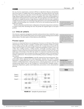
4. Consider the product structure given in Figure 5.21 per-
taining to a product manufactured by Oriental Housings
& Seals. The numbers in parentheses in the figure indi-
cates the number of units of the item required to assem-
ble one unit of its parent. Use the information available in
the product structure to answer the following questions:
(a) How many units of C are required to manufacture
one unit of Product A? Did you make any
assumption in computing this value?
(b) How much inventory of each component is
required for satisfying a demand of 100 units of
the final product if: (i) there is no stock of finished
goods (ii) there is a stock of 30 units of the final
product?
(c) Consider Problem (a). Will the computations change
if there is some stock of Item B? Why and by how
much? (Hint: Assume that you have x units of Item B
to proceed with the analysis)
5. In Problem 4, the lead times for manufacture/assembly
of the components are as follows:
Product A 2 weeks
Component B 1 week
Component C 2 weeks
Component D 2 weeks
Component E 1 week
(a) How early can Oriental deliver an order of 100 units
of the product to the customer if (i) there is no stock
of Item B (ii) there is a stock of 220 units of Item B?
(b) Will the results change if there is a stock of Product
A?
6. Given in Table 5.12 is a partially completed MRP work-
ing for Component X. Using the information provided,
complete the table.
7. Consider Component XX, for which the MRP exercise
needs to be done. The relevant information pertaining
to the component has been extracted from the com-
pany records and reproduced in Table 5.13. Currently,
E(2)
B(2)
C(2) C(4)
A
D(3)
FIGURE 5.21 Product structure for
Oriental Housings & Seals product
TABLE 5.12 Incomplete Table for Problem 6
Component X Lot Size: 2 Periods
BOM Quantity: 1 Lead Time: 1
0 1 2 3 4 5 6
Gross requirement 200 150 100 200 120 200
On-hand inventory 300
Net requirement
Planned receipts
TABLE 5.13 Data about Component XX (Problem 7)
Component XX Lot Size: ?
0 1 2 3 4 5 6
On-hand inventory 600
Net requirement
Planned receipts
Planned order
releases

160 Chapter 5
no decision has been made about the lot-sizing rule.
Company estimates suggest that the cost of carrying
inventory is `10 per unit per period and the cost of sched-
uling an order is `500 per order. The economic order
quantity is 150 units.
Use this information to analyse the following five lot-size
rules and suggest an appropriate lot-sizing rule for the
component.
(a) Lot for lot
(b) POQ = 3 periods
(c) POQ based on the economic order quantity
(d) FOQ = 500
(e) FOQ = 1,000
8. Consider the product structure of a manufacturing firm,
as shown in Figure 5.22. The company is interested in
performing an MRP exercise for the next eight weeks to
cover the requirements indicated in the MPS. The MPS
requirements for the next eight weeks are 20, 80, 100,
200, 100, 0, 120, and 150.
The relevant information on lead time, inventory status
and lot sizing are available in Table 5.14. Develop the
MRP schedule for the final product as well as for all the
components and answer the following questions:
(a) Do we need to schedule order releases for
Component B? If so, when and how much?
(b) How long will the on-hand inventory of Item D
satisfy the requirement?
(c) How many orders need to be placed for
Component F?
(d) If the cost of scheduling an order is `2,000, what is
the total cost of ordering for the MRP plan?
9. Figure 5.23 shows the product structure for a manu-
facturing firm. In addition to the final product (Product
A), Component B is sold as a spare in the market. The
MPS for Product A and Component B and other relevant
information for the problem are given in Tables 5.15 and
5.16.
Perform an MRP exercise to cover the requirements of
the MPS and answer the following questions:
(a) What is the gross requirement for Component B
during the six periods?
TABLE 5.14 Lead Time, Inventory Status, and
Lot-sizing Rules for Problem 8
Item Lead Time
(Weeks)
Inventory
Status
Lot-sizing
Rule
A 1 100 Lot for lot
B 2 200 Lot for lot
C 1 400 2 periods
D 2 1,000 3 periods
E 2 2,000 2 periods
F 2 1,200 500
G 1 2,000 1,000
TABLE 5.15 MPS for the Next Six Periods
Period 1 2 3 4 5 6
Product A 100 80 220 140 70 160
Component B 40 30 70 60 50
A
B(2)
D(2) E(2) D(4) F(2) G(2)
C(3)
FIGURE 5.23 Product structure for Problem 9
TABLE 5.16 Lead Time, Inventory Status, and
Lot-sizing Rule for Problem 9
Item Lead time
(Weeks)
Inventory
Status
Lot-sizing
Rule
A 2 200 Lot for lot
B 2 900 Lot for lot
C 1 750 Lot for lot
D 2 2,500 2 periods
E 1 300 3 periods
F 2 1,000 500
G 1 600 1,000
A
E(2) G(2)
D(3)
C(2)
F(2)
E(2)
B(2)
FIGURE 5.22 Product structure for Problem 8

(b) How many orders do we have to place for
Component C and in what quantities?
(c) Suppose the lead time for Component G is two
weeks instead of one week, what will its impact be
on the planning process?
(d) Suppose that the economic order quantity for
Component C is 320 units. What will the appropriate
POQ lot-sizing rule be for Component C?
10. Consider the following MRP (Table 5.17) for Component
C, which is used in a product manufactured by an
organization.
Of late, the organization has been experiencing frequent
shortages of this component. It has been estimated that
on an average, the company loses `5,000 by way of lost
business and goodwill due to these shortages in a six-week
period. Therefore, it has been decided to include a safety
stock of 100 units. Rework the planning details for this
component by incorporating the safety stock requirement.
11. In Problem 10, assume that the organization decided
to implement a safety lead time of one week instead of
safety stock.
(a) Rework the planning details for this component by
incorporating the safety lead time requirement.
(b) Compare the two results and list two significant
observations that you have made.
TABLE 5.17 MRP for Component C
Component C Lot Size: LFL
0 1 2 3 4 5 6
On-hand inventory 400 300 50 0 0 0 0
Net requirement 0 110 0 200 70
Planned receipts 0 110 0 200 70
Planned order
releases
110 0 200 70 0
1. Visit the Web sites of the major ERP vendors (SAP,
PeopleSoft, Oracle, Ramco, J.D. Edwards). Study the prod-
uct offerings of all these vendors and prepare a detailed
report to answer the following questions:
(a) What are the key components of the ERP system
offered by the major vendors?
(b) How do these vendors differentiate differ their
offerings?
(c) If an organization wishes to choose one of the
four vendors, what factors will you suggest to the
organization to enable appropriate selection?
(d) Are there industry-specific offerings of ERP by these
vendors? If so, which sectors of the industry are
covered and how well?
E
N E X
T E
- R
W I S E C I S E S
1. Take a simple household gadget or appliance such as a din-
ing table set or a sofa set with a centre table. Carefully ana-
lyse the assembly of the appliance and identify the parts that
make up the appliance. Identify the major assemblies and
sub-assemblies of the appliance.
(a) Using this information prepare a complete BOM
and a product structure for the appliance
(b) What are the various ways by which you think
product varieties can be created for this appliance?
Identify them and prepare an indented BOM for the
entire set of product offerings.
(c) Assume an MPS and other relevant data for the
components that you have identified for the
appliance. Can you set up a standard table for
performing the MRP exercise for the appliance?
2. Set up the table created in Problem 1 in a Microsoft Excel
worksheet (assume a planning horizon of 6 periods). Use
the worksheet to accomplish the following tasks:
(a) Perform the MRP exercise for the appliance that you
have chosen.
(b) Assume that the MPS is wrong. Quantities have been
underestimated to the extent of 10 per cent during
Periods 4 and 5 and overestimated to the extent of 5
per cent during Period 6. What is the likely impact of
this on customer commitment?
R
N J
I O
I E C
P T
M S

162 Chapter 5
5-1. Operating inventories are dependent on:
A. Supply
B. Demand
C. Production
D. Procurement
5-2. What are the two types of inventories exist in an
operating system?
A. Operating and distribution inventories
B. Product and operating inventories
C. Distribution and product inventories
5-3. A structured approach that develops schedules for
launching orders for materials in any manufacturing
system and ensures the availability of these at the
right time and the right place is:
A. Capacity requirement planning
B. Inventory requirement planning
C. Material requirement planning
D. Production requirement planning
5-4. Regeneration is one method to update:
A. Service requirements planning schedule
B. Inventory requirement planning schedule
C. Capacity requirement planning schedule
D. Material requirements planning schedule
5-5. What is the technique that applies the MRP logic to
address the capacity issues in an organization?
A. Capacity Requirements Planning
B. Material Requirements Planning
C. Distribution Requirement Planning
D. Energy Requirement Planning
5-6. To plan distribution inventories in the downstream
supply chain, consisting of depots and stocking
points at the dealer level is termed as:
C. Energy Requirements Planning
D. Distribution Requirements Planning
5-7. The iterative process of computing all requirements
at a particular level and then moving down one level
is known as:
A. Level by level analysis
B. Top to bottom approach
C. Scheduling
D. Explosion
5-8. Which is that organization-wide planning system
that utilizes some common software and an inte-
grated database for planning and control purposes?
C. Energy Requirements Planning
D. Distribution Requirements Planning
5-9. In which of the below, planning is based on resources?
B. Resources Planning in Services
C. Distribution Requirements Planning
D. Service Requirements Planning
5-10. What are the two types of inventories exist in an
operating systems?
A. Operating inventory and distribution inventory
B. Fixed inventory and fluctuation inventory
C. Physical inventory and computerized inventory
D. First in First out and Last in Last out
Answer Keys: 5-1. B 5-2. A 5-3. C 5-4. D 5-5. A 5-6. D 5-7. D 5-8. C 5-9. B 5-10. A
Notes

Notes

164
C H A P T E R
CRITICAL
QUESTIONS
6
Inventory Management
and Models
• What are the various types of inventory found in an organization?
• What are the costs and decisions related to inventory management?
• How is economic order quantity computed?
• How can one model demand uncertainty and compute appropriate levels of investment
to be made in inventory?
• What are the alternative inventory management systems in use in organizations?
• What are the alternative approaches available for selective control of inventories?
• How is inventory planning done in the case of a single-period demand?
Organizations need to spend a
considerable amount of money to
carry inventory. The cost of stores and
warehousing and the administrative
costs related to maintaining inventory
and accounting for it form a significant
part of this cost.
Source: MTR Foods Pvt. Ltd.

Inventory Management and Models 165
Inventory Management in a Consumer Products Company
A consumer products company dealing in
cosmetics and other personal-care products
was exploring ways to reduce inventory levels across
their outbound supply chain and improve inventory
record accuracy at their storage points. The company
had a supply chain network of three factories with
bonded stock rooms (BSRs) attached for dispatch to the
depots and 35 depots for servicing distributors. Goods
moved from the factory to the BSRs. The BSRs dis-
patched stocks to one centralized depot. Other depots
received stocks from this depot and sold them to dis-
tributors.
These depots were holding high levels of inven-
tory of old/withdrawn stocks and damaged stocks for a
long time (over three months). The total average inven-
tory holding at the BSRs was 8.2 weeks of sales and at
the depots was 6.5 weeks of sales. There were several
reasons for high levels of inventory. Some of them are
discussed here.
Sales and dispatch forecasts were not in line with
actual sales. Furthermore, there was no process to peri-
odically review and refine the annual forecasts utilizing
market feedback. Stocking across all points in the dis-
tribution chain was driven by a push-oriented system
that did not have any provision for factoring in market
requirements. Actual safety stocks maintained at depots
were significantly higher than the target safety stocks
agreed on at the beginning of the operating year. No
system was in place to monitor and correct this prac-
tice. There was also a high level of old/damaged/slow-
moving stocks. Dead stock was allowed to accumulate
in the system mainly because there was an absence of
visibility into inventory details across stocking points.
The process to monitor and act on dead stock was not
adhered to and records of slow-moving/old/damaged
stocks were not maintained methodically at the stock-
ing points.
A study was conducted focusing on the inven-
tory-related issues at the BSRs and depots. This
included inventory holding as a proportion of sales,
practices employed for tracking goods in the ware-
house, and the proportion of fast- and slow-moving
stocks to the total inventory. The study also looked at
the inventory planning process pertaining to forecast
accuracy, the process of reviewing and revising fore-
casts, the level of safety stock at each location, com-
bined with the process to review and reset the same
An IT solution was implemented for computing
the forecast using consolidated orders, with factoring
for promotions and seasonality. The IT solution also
enabled the organization to calculate safety stock levels
based on the number of weeks of sales target. Demand
planning and forecasting were made a periodic activity
using the IT solution to align forecasting with market
orders and actual sales. The process of setting safety
stocks at depots was made periodic and dynamic, based
on updated sales data. Furthermore, norms were set to
act on damaged/old and other dead stocks. Clear steps
were laid down regarding the liquidation or destruction
of these stocks. An accountability chain was set up in
the organization to monitor and authorize activities in
this regard, based on the visibility provided by the IT
solution.
The overall benefit of the exercise was that the
organization was able to ensure availability of fresh
stocks in the market. This was achieved mainly by reduc-
ing inventory levels across the chain and also through
better stock management at the depots. The company
achieved a stock-level reduction from 8.2 weeks to
5.5 weeks at the BSRs and from 6.5 weeks to 4 weeks
at the depots. Transparency of saleable and damaged
stocks quantities across the supply chain resulted in
more accurate demand planning, stock allocation, and
production.
Source: K. Ravichandran and Debjyoti Paul, “Best Practices in
Inventory Management,” http://forumcentral.sify.com/athena/
login/casestudyinventory.pdf. Last accessed on 15 December 2008.
ideas
at Work
6.1
Notes

166 Chapter 6
T
he term inventory refers to any idle resource that can be put to some future use.
Manufacturing and several service organizations have significantly invested in inven-
tory. Often, investment in inventory has a direct bearing on the profitability of a
firm. Experiences in the last twenty years suggest that the world-class performance of a firm
hinges on the firm’s ability to cut investment in inventory to very low levels. Automobile
assembly plants and component manufacturers are known to carry very little inventory
and yet provide good quality finished goods at the right time. In addition to cutting down
cost, reduced inventory levels help an organization improve quality, planning systems,
and supply chain coordination. They also reduce wastage and obsolescence. Hence, inven-
tory planning and control continues to derive considerable attention of the management in
organizations.
6.1 INVENTORY PLANNING FOR INDEPENDENT DEMAND ITEMS
In manufacturing organizations, finished goods and spare parts typically belong to the category
of independent demand items. While planning for a dependent demand item is done to meet
manufacturing requirements, in the case of independent demand items, it is done to meet cus-
tomer requirements. Two attributes characterize and distinguish independent demand items:
They are in continuous demand, and there is an element of considerable uncertainty in the
demand for such items.
Continuous Demand
Independent demand items are in continuous demand. Consider the sale of consumer appliances
of manufacturers such as Videocon or LG. The demand for 32” LCD colour television panels in
a particular city will be continuous. When there is a continuous demand for an item, constant
availability of items and periodic replenishment of stock are important elements of the planning
process. Non-availability of items translates into lost sales, poor customer goodwill, and addi-
tional costs in servicing the promised deliveries.
Uncertainty of Demand
There is an element of considerable uncertainty of demand in the case of independent demand
items. On the other hand, in the case of dependent demand items, the demand is always derived
and hence known with certainty. For example, the number of tyres required per month for new
vehicles is known accurately once the monthly production is finalized. However, the number
of spark plugs required for sale as spare parts needs to be estimated on some basis. Therefore,
inventory planning for independent demand items should include some cushion for handling
uncertainties whenever they are significant.
Given these requirements, inventory planning of independent demand items must address
the following two key questions:
(a) How much? Good inventory planning must devise means by which the planner can contin-
uously replenish the stock as it depletes over time. The replenishment could be of a fixed
quantity or variable. It could be based on the costs associated with inventory. It could
also satisfy certain practical considerations such as truck capacity, quantity discounts,
and minimum order quantity restrictions posed by the supplier.
(b) When? The other issue is the timing of replenishment. Since demand is continuous and
uncertain, the timing of replenishment is equally crucial. There are numerous ways of
addressing the timing. It could be based on consumption patterns, the value of the item,
managerial preferences for review, and other practical considerations.
The term inventory denotes
any idle resource that could be
put to some future use.
In manufacturing organizations,
finished goods and spare parts
typically belong to the category
of independent demand items.
Inventory planning of
independent demand items
must address the two key
questions: how much, and
when?
Notes

6.2 TYPES OF INVENTORY
Before planning for inventory, it is important to know why organizations carry inventory and
what factors influence the level of investment. Five types of inventory are normally found in
most organizations.
Seasonal Inventory
Organizations carry inventory to meet fluctuations in demand arising out of seasonality. During
festival periods, the demand for consumer durables may be high due to an increase in dispos-
able income in the hands of consumers. In order to meet this surge in demand, there is inven-
tory build-up during non-peak periods. Similarly, in a fast-food restaurant, a certain amount of
inventory build-up happens during non-peak hours to handle the increase in demand during
peak hours. In both these cases, inventory plays the crucial role of addressing short-term capac-
ity issues in an organization.
Decoupling Inventory
Manufacturing systems typically involve a series of production and assembly workstations.
Raw material passes through these stages before it is converted into finished goods. Each stage
behaves idiosyncratically on account of varying process times, downtimes, and resource avail-
ability. Therefore, the planning and control of such multi-stage production processes becomes
very complex. One way to simplify the production planning and control problem is to decou-
ple successive stages using inventory at some intermediate points. Each stage will have an input
buffer and an output buffer. The output buffer of the preceding stage becomes the input buffer of
the succeeding stage. Inventory decisions in this case require analysis of workstation capacities,
resource availability, and bottlenecks.
Figure 6.1 illustrates the use of decoupling inventory. In the first case, there is no decoupling
inventory. In this case, all the ten stations of production are to be closely monitored and flow
balance is to be ensured on a continuous basis. If there is a problem in one of the stations, it will
affect all upstream and downstream stations. Further, the vagaries of demand uncertainty will
directly affect the system’s performance. Planning and control is challenging, especially when
the number of stations is very large. On the other hand, the second case in Figure 6.1 has decom-
posed the production into three major stages. Each stage is linked to the other using decoupling
inventory. This enables each stage to work with reasonable levels of independence. Further, the
adverse impact of one stage will not immediately affect the others. Therefore, a certain amount
of decentralized planning and control is possible.
Five types of inventory
are normally found in
organizations: seasonal
inventory, decoupling inventory,
cyclic inventory, pipeline
inventory, and safety stock.
Production system without any decoupling inventory
Decoupling inventory
Stage 1 Stage 2 Stage 3
1 2 3 4 5 6 7 8 9 10
1
2
3
4 5
6 7
8 9
10
FIGURE 6.1 An illustration of the use of decoupling inventory
Notes

168 Chapter 6
Cyclic Inventory
It is customary for organizations to order inventory in repeated cycles and con-
sume them over time. For example, a hospital may order disposable syringes
in quantities of 10,000. If the average consumption rate is 500 per day, then it
takes 20 days to deplete one order. On the twenty-first day, another order of
10,000 will arrive and it will be consumed over the next 20 days, and so on.
Cyclic inventory goes through a saw-toothed pattern as shown in Figure 6.2.
Each cycle begins with replenishment and ends with complete depletion of the
inventory.
If Q is the order quantity per cycle,
The average cyclic inventory =
Q Q
+
=
0
2 2
(6.1)
Pipeline Inventory
Pipeline inventory pertains to the level of inventory that organizations carry in the long run due
to non-zero lead time for order, transport, and receipt of material from the suppliers. Because of
the geographical distances between the buyers and the suppliers and the host of business pro-
cesses involved in ordering and receiving material, there is a time delay between order place-
ment and order receipt. The inventory carried to take care of these delays is known as pipeline
inventory.
Consider the example of the hospital. Suppose it takes three days to supply disposable syringes.
Then the hospital should place an order at the end of Day 17 in order to replenish the stock to
10,000. This means that an order will be placed when the inventory level reaches 1,500 (3 days at
the rate of 500 syringes per day). In general, if the lead time for supply is L, and the mean demand
per unit time is m, then the pipeline inventory is L × m.
In the long run, the system will always have this inventory in order to take care of lead time
for supply. The only way organizations can reduce this inventory is to cut down lead time for
procurement, production, and distribution. Locating suppliers nearby, re-engineering the busi-
ness processes related to procurement and distribution of materials, and
using efficient alternatives for logistics are some of the ways in which an
organization can reduce lead time and pipeline inventory.
Safety Stock
Organizations also have additional investment in inventory to buffer
against uncertainties in demand and supply of raw material and compo-
nents. We know from the elementary theory of probability distributions
that when demand is stochastic, carrying average inventory will ensure
that the demand is met only 50 per cent of the time (in the long run).
However, in order to improve the availability to meet uncertain demand,
an additional quantity known as safety stock is kept. Greater investment
in safety stock leads to a lower probability of inventory going out of stock.
Similarly, the higher the uncertainty, the greater is the need for safety stock.
Safety stock only serves to prevent shortages in the short run. However, in
the long run, the demand will tend toward an average value and the safety
stock will not be consumed. Figure 6.3 represents an inventory system
with safety stock and other types of inventory.
Reducing safety stock calls for reducing uncertainty in the system.
Investment in superior planning and forecasting systems and good
Time
Quantity
FIGURE 6.2 Cyclic inventory
Cyclic
inventory
Lead
time
Pipeline inventory
Safety stock
Time
Quantity
FIGURE 6.3 Cyclic inventory, pipeline
inventory, and safety stock

supplier development practices will help organizations reduce uncertainty in the system. In the
case of components manufactured in-house, better production planning and improved mainte-
nance of resources will help reduce uncertainty in the system.
Cyclic inventory, pipeline inventory, and safety stock are critically linked to both the “how
much” and “when” questions in inventory planning. Lead time influences the “when” decision
directly and determines the level of pipeline inventory in the system. Similarly, cyclic inventory
is the outcome of the “how much” decision that an inventory planner makes. Safety stock influ-
ences both “how much” and “when” in an indirect sense. However, in order to understand how
these decisions are made, one needs to understand various costs associated with inventory plan-
ning and control.
6.3 INVENTORY COSTS
There are several costs associated with inventory planning and control. These costs could be clas-
sified under three broad categories:
➱ The cost of carrying inventory. All costs related to maintaining inventory in organizations
will be classified under this.
➱ The cost associated with ordering material and replenishing it in cyclic intervals.
➱ The cost arising out of shortages.
Inventory control models should take these into consideration and aim at minimizing the sum of
all these costs. Sometimes, the unit cost of the item for which inventory planning is done is also a
relevant cost for decision making. This is because when large quantities are ordered, there could
be some discount in the unit cost of the item.
Inventory-carrying Cost
Organizations need to spend a considerable amount of money to carry inventory. The most sig-
nificant component is the interest for the short-term borrowals for the working capital required
for inventory investment. The second significant cost relates to the cost of stores and warehous-
ing and the administrative costs related to maintaining inventory and accounting for it. The ele-
ments of storing and warehousing costs include the following:
➱ Investment in store space and storage and retrieval systems
➱ Software for maintaining the inventory status
➱ Managerial and other administrative manpower to discharge various activities related to
stores
➱ Insurance costs
➱ Cost of obsolescence, pilferage, damages, and wastage
Reducing safety stock calls for
reducing uncertainty in the
system.
Cyclic inventory, pipeline
inventory, and safety stock are
critically linked to the “how
much” and “when” questions in
inventory planning.
A manufacturer of transformers requires copper (both
in plate and wire form) as a key ingredient. The average
weekly requirement of copper is 200 tonnes. The lead time
for the supply of copper is two weeks. If the manufacturer
places monthly orders of copper, analyse the various types
of inventory in the system.
Solution
Order quantity Q=1 month requirement=800 tonnes.
Cyclic inventory in the system=
Q
2
800
2
400
= = tonnes.
Lead time L = 2 weeks
Average weekly demand m = 200 tonnes
Pipeline inventory=L×m = 200 × 2 = 400 tonnes.
EXAMPLE 6.1
Notes

170 Chapter 6
In the case of high-tech electron-
ics and short-shelf-life items, such
as active chemical compounds,
food items, and pharmaceutical
formulations, obsolescence costs
could be significant. Table 6.1
shows a sample computation of
carrying cost for a company. The
components of inventory-carry-
ing costs exert considerable pres-
sure on an organization to keep
inventory levels low. However,
the ability of an organization to
reduce inventory depends on the
nature of business processes in
place, the lead time for procure-
ment, and the quality of plan-
ning, as pointed out in the earlier
section.
Note that all the costs related
to carrying inventory are directly
related to the level of inventory.
Graphically, it can be shown as a
simple linear relationship (Figure
6.4). Let Cc denote the inventory-
carrying cost per unit per unit time. Since the interest component is the predominant part of Cc,
the usual practice is to represent Cc as a percentage of the unit cost of the item. Thus, if Cu is the
unit cost of the item, then Cc = iCu, where i is in percentage. For example, if the unit cost of an
item is `5,000, the annual interest charges are 12 per cent, and the other annual costs related to
carrying inventory are 3 per cent, then the inventory-carrying cost is 15 per cent of the unit cost,
that is, `750 per unit per year.
For an order quantity of Q, the average inventory carried by an organization is Q/2. Therefore,
Cost associated with carrying inventory
=
Q
Cc
2
×
⎛
⎝
⎛
⎛
⎛
⎛
⎝
⎝
⎛
⎛
⎛
⎛ ⎞
⎠
⎞
⎞
⎞
⎞
⎠
⎠
⎞
⎞
⎞
⎞ (6.2)
Cost of Ordering
Replenishment of cyclic inventory is achieved by ordering material with the suppliers.
Organizations perform a series of tasks related to ordering material. These include search
and identification of appropriate sources of supply, price nego-
tiation, contracting and purchase-order generation, follow-up
and receipt of material, and eventual stocking in the stores after
necessary accounting and verification. In Chapter 7, we have dis-
cussed several aspects pertaining to this in some detail. All these
tasks involve manpower, resources, and time that can be classi-
fied under cost of ordering. Since several of these costs are fixed in
nature, ordering a larger quantity could reduce the total costs of
ordering. A larger order quantity Q will require fewer orders to
meet a known demand D, and vice versa. The relationship between
Q and the total cost of ordering is graphically shown in Figure
6.4. Table 6.2 shows a sample computation of ordering cost for a
company.
The number of orders to be placed to satisfy a demand of D =
D/Q. If C0 denotes the cost of ordering per order, then:
Total ordering cost =
D
Q
C
×
⎛
⎝
⎜
⎛
⎛
⎝
⎝
⎞
⎠
⎟
⎞
⎞
⎠
⎠
0 (12.3)
TABLE 6.1 Computation of Carrying Cost: An
Illustration
Sl. No. Item of Expenditure (Annual) Amount (`)
1 Stationary 75,000.00
2 Insurance premium 375,000.00
3 Establishment expenses and
overheads
275,000.00
4 Salary of stores personnel 1,100,000.00
Total expenditure 1,750,000.00
Average value of the inventory
in stores
35,000,000.00
Warehousing cost (in %
inventory value)
5.00%
a Cost of warehousing 5.00%
b Cost of capital (assumed) 15.00%
c Obsolescence (estimated
historically)
2.00%
d Damages, spoilage, etc.
(estimated historically)
1.00%
Carrying cost (%) 23.00%
Sum of the costs
Total cost of carrying
Total cost of ordering
Minimum cost
Level of inventory
Economic
order quantity
Total
cost
FIGURE 6.4 Behaviour of ordering and carrying
costs of inventory
Notes

Sometimes, components required for
use in an organization are sourced
from within. A division or a depart-
ment of the organization may be
specially manufacturing the required
componentsforinternalconsumption.
In such situations, the costs associated
with setting up the required machin-
ery will represent the cost of order-
ing. For example, let us assume that a
component is produced in-house. In
order to manufacture the component,
two machines are to be set up and it
takes 60 minutes and 120 minutes
respectively in these machines. It also
requires consumables and tools for
the purpose of setting up the machine.
Finally, direct labour time and super-
visor time needs to be devoted for the
activity. By estimating the cost of all
these factors, we can arrive at the cost
of set-up.
The cost of carrying and the cost of ordering are fundamentally two opposing cost struc-
tures in inventory planning. For instance, when the order quantity becomes smaller, the total
cost of carrying inventory decreases. On the other hand, since a large number of orders are to
be placed to satisfy the demand, the total ordering costs will go up. Conversely, when the order
quantity is increased, while the total cost of ordering will come down owing to fewer orders
being placed, the total cost of carrying inventory will increase due to an increase in the average
cyclic inventory in the system. Balancing these two opposing costs will be central to inventory
planning and control in any organization. Figure 6.4 gives a graphical representation of the
sum of these two costs.
Cost of Shortages
Despite careful planning, organizations are likely to run out of stock for several reasons. There
could be a sudden surge in demand. Alternatively, the suppliers might not have delivered the mate-
rial as per schedule, or a lot could have been rejected because of defective components. Such events
disrupt production and have a cascading effect down the supply chain. Delivery schedules are
missed, leading to customer dissatisfaction and loss of goodwill. It also introduces additional costs
arising out of pushing the order back and rescheduling the production system to accommodate
these changes. Rush purchases, uneven utilization of available resources, and lower capacity utili-
zation further escalate the costs in the system. All these form part of the cost of shortage.
The cost of shortage per unit is denoted by Cs. Since the effects of shortage are vastly intan-
gible, it is difficult to accurately estimate Cs. In practice, managers tend to use other measures to
incorporate the cost of shortage if estimation of Cs proves to be futile.
6.4 INVENTORY CONTROL FOR DETERMINISTIC DEMAND ITEMS
Let us consider a situation in which the demand for an item is continuous and is known with cer-
tainty. Since the demand is known, we exclude the possibility of having shortages. Better inven-
tory control requires that we answer the “how much” and “when” questions by balancing the
total costs of carrying inventory and ordering. For an order quantity of Q, we can compute the
total cost of carrying and ordering from Eqs. 6.2 and 6.3.
Total cost of the plan = Total cost of carrying inventory + Total cost of ordering
TC Q
Q
C
D
Q
C
c
( )
Q = +
Q
Cc
2
0
⎛
⎝
⎛
⎛
⎝
⎝
⎞
⎠
⎞
⎞
⎠
⎠
×
⎛
⎝
⎜
⎛
⎛
⎝
⎝
⎞
⎠
⎟
⎞
⎞
⎠
⎠
(6.4)
When the total cost is minimum, we obtain the most economic order quantity (EOQ).
The cost of carrying and
the cost of ordering are
fundamentally two opposing
cost structures in inventory
planning.
TABLE 6.2 Computation of Ordering Cost: An
IIustration
Sl. No. Item of Expenditure
(Annual)
Amount (`)
1 Stationary 80,000.00
2 Telephone 40,000.00
3 Other communication
expenses
60,000.00
4 Salary of purchase
department personnel
1,100,000.00
5 Inwards goods inspection
section expenses
350,000.00
6 Other expenses and
overheads
200,000.00
Total expenditure 1,830,000.00
No. of purchase orders
generated
600.00
Average cost of ordering 3,050.00
Notes

172 Chapter 6
By taking the first derivative of Eq. 6.4 with respect to Q and equating it to zero, we can obtain the
EOQ. Differentiating Eq. 6.4 with respect to Q we obtain:
dTC Q
dQ
C C D
Q
c
( )
Q
= −
2
0
2
⎛
⎝
⎛
⎛
⎝
⎝
⎞
⎠
⎞
⎞
⎠
⎠
Note that the second derivative is positive and hence we obtain the minimum cost by equating
the first derivative to zero. Equating the first derivative to zero and rearranging the terms, we
obtain Eq. 6.5.
Denoting EOQ by Q*
, we obtain the expression of Q* as:
Q
C D
Cc
* =
2 0
(6.5)
Optimal number of orders =
D
Q* (6.6)
Time between orders =
Q
D
*
(6.7)
Q*
answers the “how much” question directly. Every time the inventory depletes to zero, it is
economical to place an order equal to Q*
. Similarly, time between orders answers the “when”
question. Since the demand is continuous, the demand rate will determine “when” to place an
order. For instance, if the annual demand for an item is 2,500 units and if there are 250 working
days, the daily demand is 10. If Q*
is 300, then it is implied that an order needs to be placed every
30 days.
A two-wheeler component manufacturing unit uses large
quantities of a component made of steel. Although these
are production items, the demand is continuous and
inventory planning could be done independent of the
production plan. The annual demand for the component is
2,500 boxes. The company procures the item from a sup-
plier at the rate of `750 per box. The company estimates
the cost of carrying inventory to be 18 per cent per unit
per annum and the cost of ordering as `1,080 per order.
The company works for 250 days in a year. How should the
company design an inventory control system for this item?
What is the overall cost of the plan?
Solution
Annual demand for the item (D) = 2,500 boxes
Number of working days = 250
The average daily demand =
2500
250
= 10 boxes
Unit cost of the item (Cu) = `750.00 per box
Inventory-carrying cost = iCu = 0.18 × 750.00 =
`135.00 per unit per year
Cost of ordering (C0) = `1,080.00 per order
The “how much” decision:
Economic order quantity(Q*
)
= =
× ×
=
2 2 1080 2500
135
200
0
C D
0
Cc
Boxes
Number of orders to be placed
= = =
D
Q*
.
2500
200
12 5 1
≅ 33
The “when” decision:
Time between orders
= = = × =
Q
D
250
2500
0 08 0
= 08 250 20
.
0
.08 .
yea days
Total cost of the plan
Hence, the manufacturer will place an order for 200
boxes of the component once in every 20 days and will
incur a total cost of `27,000 for the plan. Any quantity
above or below will increase the cost of the plan.
EXAMPLE 6.2
Notes

Problems in the EOQ model
We have made several assumptions while deriving Q*
. The salient among these include the
following:
(a) The demand is known with certainty and is continuous over time.
(b) There is an instantaneous replenishment of items.
(c) The items are sourced from an external supplier.
(d) There are no restrictions on the quantity that we can order.
(e) There are no preferred order quantities for the items.
(f) No price discount is offered when the order size is large.
In practice, several of these assumptions do not hold. Despite this, the EOQ model can be applied
with suitable modifications because it is robust. Because of the square root in the formula, changes
in model parameters, such as demand and cost, have less impact on the solution. If demand is not
known accurately, one can use representative figures for D and assess the impact of changes on the
total cost of the plan (see Problem 4 at the end of the chapter). The assumption of instantaneous
replacement can be easily taken care of by placing an order ahead. If the lead time is L, then by
placing an order L periods ahead of depletion of inventory, one can ensure availability of mate-
rial. Similarly, if the items are manufactured in-house, it is possible to estimate the economic run
length by a simple modification to Eq. 6.5.
Assumptions (d), (e), and (f) indicate the need for examining the suitability of utilizing order
quantities different from Q*
. Large order sizes result in price discounts. There are other rea-
sons for placing a larger order than what the EOQ suggests. Sometimes, it will be economical
to transport a truckload of items and save on transportation cost. In other cases, the supplier
may impose a minimum order quantity. In all these cases, the relevant cost for analysis includes
cost elements other than carrying and ordering. An analysis of these relevant costs will help the
inventory planner make an appropriate choice in order quantity. See Example 6.3 for an illustra-
tion of this.
The EOQ model is robust
and can be applied in several
real-life settings with some
modifications.
Consider Example 6.2. Assume that the carrying cost of the
component remains `135 per unit per year and that the
supplier is willing to offer a discount on the unit price as
per the following structure:
Up to 399 boxes = No discount
400 − 799 boxes = 2 per cent discount
800 − 1,000 boxes = 3 per cent discount
What should the company do in this case?
Solution
The economic order quantity is 200 boxes and the unit
price of the item is `750.
There are two other order quantities at which the unit
price changes on account of discount.
At Q1 = 400, unit price of the item = 0.98 × 750 =
`735.00
At Q2 = 800, unit price of the item = 0.97 × 750 =
`727.50
Since there is a discount on the price as the order quan-
tity is varied, the total cost comparison between alternatives
can be made only after incorporating the purchase price.
Total cost for Q*
Total cost for Q1
Total cost for Q2
cost for Q2
Since TC(Q1) is the lowest among the alternatives, the firm
can make use of the discount offered and reset the order
quantity to 400 boxes.
EXAMPLE 6.3

174 Chapter 6
6.5 HANDLING UNCERTAINTY IN DEMAND
With some modifications, the EOQ model can accommodate several practical considerations.
However, when the demand is uncertain, instances of shortages occur while operating the sys-
tem with EOQ. There are two ways of handling the issue of shortages. One is to incorporate
shortage cost in the model. The other is to use the concept of service level. Service level is the
desired probability of not running out of stock between the time an order is placed with a sup-
plier and the order is received. For example, if an organization wants to operate with a 90 per cent
service level, it means that in the long run, the organization is able to meet the demand on 90 per
cent of all occasions.
Consider an item with uncertain demand. When the item is available in stock, there is no risk
of shortage. However, when an order is placed, the demand can be met only with the available
stock until the stock is replenished by an order. Hence, if an organization is protected from the
risks of shortage during the supply lead time, then inventory planning is better. The concept
of service levels seeks to achieve this objective. Let us understand the concept of service level
through a simple example.
Consider an item with uncertain demand that has a lead time of one week. Based on observed
consumption patterns one can estimate the weekly demand. Table 6.3 has illustrative data for
the item. The last two columns show the cumulative frequency of demand exceeding the lower
class. For example, the weekly demand exceeded 30 units during 98.25 per cent of the observed
occasions and exceeded 180 units during 18.42 per cent of the occasions. The information in the
table can also be plotted as a frequency ogave (see Figure 6.5).
From the data, one can compute the average demand during lead time to be 143 units. If the
organization stocks 143 units at the time of placing the order with the supplier, then in the long
run, it will be able to meet the demand during lead time only on 50 per cent of the occasions.
In other words, the organization has a 50 per cent service level if it operates with this inventory
level. Clearly, this will be an undesirable situation and managers would want to offer better ser-
vice. From the data, we can compute the number of units to be stocked to offer 90 per cent and
95 per cent service levels to be 203 and 224 units, respectively. By stocking 60 more units (203–
143), the organization can improve the service level from 50 per cent to 90 per cent. Similarly,
by investing an additional 21 units, it can further increase the service level to 95 per cent. This
additional stock is known as “safety stock” because it provides the needed safety to an organiza-
tion to handle uncertain demand during lead time.
Service level is the desired
probability of not running out
of stock between the time an
order is placed with a supplier
and the order is received.
TABLE 6.3 The Service Level Concept: An Illustration
Demand Exceeding Lower Class
Demand During Lead Time Frequency of Occurrence Cumulative Frequency Cumulative Percentage
0–30 2 114 100.00%
31–60 5 112 98.25%
61–90 11 107 93.86%
91–120 20 96 84.21%
121–150 25 76 66.67%
151–180 30 51 44.74%
181–210 13 21 18.42%
211–240 5 8 7.02%
241–270 2 3 2.63%
271–300 1 1 0.88%
Notes

The concept of service levels permits managers to sidestep problems related to estimating
shortage cost per unit. Using this concept, it is possible for managers to relate the amount of
additional investment required and the improvement in service and strike appropriate trade-
offs between additional investment and service. In the example we just discussed, a 5 per cent
increase in service level from 90 per cent to 95 per cent entails an additional investment of 21
units. Depending on the unit cost of the item in question, the cost of carrying and the competi-
tive scenario, managers can strike a better trade-off in their choice towards the appropriate level
of service that needs to be offered.
These computations can be generalized by using a few notations and replacing the empirical
distribution for demand by a theoretical distribution such as normal distribution.
Let the demand during lead time follow a normal distribution with:
m(L), the mean demand during lead time and
s(L), the standard deviation of demand during lead time
Let (1 – a) denote the desired service level, where a denotes the probability
of a stockout.
Za is the standard normal variate corresponding to an area of (1 –a) cov-
ered on the left side of the normal curve.
An expression for safety stock (SS) is given by SS = Za × s(L).
Figure 6.6 represents the principle of safety stock and service level.
Due to the introduction of safety stock, the total cost of the plan will change.
The total cost for an order quantity equal to Q*
is given by:
Total cost of the plan = Cost of ordering + Cost of carrying cyclic inven-
tory + Cost of carrying safety stock
TC Q
D
Q
C
Q
Cc
( *
Q )
*
*
×
=
⎛
⎝
⎛
⎛
⎝
⎝
⎞
⎠
⎟
⎞
⎞
⎠
⎠
×
Q
+
⎛
⎝
⎛
⎛
⎝
⎝
⎞
⎠
⎞
⎞
⎠
⎠
( )
C
a c
C
( )
Za
Z ( )
L
L
Za
Z ×
0
2
(6.8)
The concept of service level
permits managers to sidestep
problems related to estimating
shortage cost per unit.
100%
95%
90%
85%
80%
75%
70%
65%
60%
55%
50%
45%
40%
35%
30%
25%
20%
15%
10%
5%
0%
0 30 60 90 120 150 180 210 240 270 300
Cumulative
percentage
Demand for the item
FIGURE 6.5 Frequency ogave of weekly demand
m(L)
a = 10%
Za
× s(L)
Mean demand
during
lead time
Safety stock for
90% service level
FIGURE 6.6 Illustration of service level
and the safety stock concept
Notes

176 Chapter 6
If the organization places an order when the stock on hand is equal to the sum of mean demand
during lead time and safety stock, then it will be able to provide a service level of (1 – a) in the
long run. Therefore, an expression for reorder point (ROP) for systems with uncertain demand
is given by:
ROP = m(L) + Za × s(L) (6.9)
6.6 INVENTORY CONTROL SYSTEMS
The previous sections provide organizations with the necessary building blocks to put inven-
tory control systems in place. In practice, organizations employ some methods to manage and
control inventory. Prominent among them include the use of continuous review of inventory
and periodic review of inventory. Let us understand the working of these two systems, and also
how various decision parameters of these systems can be estimated using the building blocks
provided in previous sections.
The Continuous Review (Q) System
Organizations widely use a continuous review system called a two-bin system. In operation, the
available inventory is stocked in two bins, first in a smaller bin and the balance in a larger bin. As
the material is consumed, the larger bin is emptied first. As soon as the larger bin is empty, an
order is placed with a supplier for a predetermined quantity, Q, and until the material arrives in
the stores, the smaller bin is consumed. During replenishment, the smaller bin is filled in first and
the cycle continues. Can you guess what will be the capacity of the smaller bin? A little thought
will help you appreciate that the capacity of the smaller bin is indeed the reorder point as per the
calculations that we performed in the previous section.
Figure 6.7 shows the general working of a Q system. The inventory position in the system is
continuously monitored to check if it has reached the reorder point. Once it reaches the reorder
The daily demand for an item is stochastic and follows the
normal distribution with a mean of 100 and a standard
deviation of 20. The supplier of the item takes two weeks
to deliver the item from the date the order is placed. What
will be the appropriate reorder point for 90 per cent and
95 per cent service level? The cost of ordering is `1,000 per
order and the carrying cost is `250 per unit per year. There
are 250 working days in a year. If the organization places
orders in fixed quantities of 500, what will be the total cost
of the plan?
Solution
Mean daily demand = 100
Number of working days in a year = 250
Total annual demand = 25,000
Lead time for supply (L) = 2 weeks = 14 days
Therefore, mean demand during LT, m(L) = 14 × 100
= 1,400
Standard deviation of daily demand = 20
Variance of daily demand = 400
Variance of the demand during LT = 14 × 400 = 5,600
Standard deviation of demand during LT, s(L) = 74.83
For 90 per cent service level, a = 10 per cent and
(1 – a) = 90 per cent.
From standard normal tables (Za) = 1.28
Safety stock (SS)=Za×s(L)=1.28×74.83=95.78 ≈ 96
Therefore, ROP=m(L)+Za×s(L)=1,400+96=1,496
Total cost of the plan,
For 95 per cent service level, the corresponding values are:
a = 5 per cent, (1 – a) = 95 per cent and Za = 1.645, SS
= 123.09 ≈ 124 and ROP = 1,400 + 124 = 1,524.
Total cost of the plan
EXAMPLE 6.4
Notes

point, an order is placed for a fixed quantity of Q. Due to this design choice of ordering fixed
quantities, Q systems are also known as fixed order quantity systems. After a lead time of L, the
inventory arrives in the system and the physical inventory increases. In Figure 6.7, the continuous
line indicates the on-hand inventory in the system. When there is a pending order, the physical
inventory in the system is less but the total inventory in the system must take into consideration
scheduled receipts in the future. This is shown by the dotted line of inventory movement. The
two constant dotted lines in the bottom of the figure represent the safety stock built into the
system and the average demand during lead time (LT). The summation of these two quantities is
the reorder point for the system.
The “when” decision is answered by ROP. We can employ the computations in the previous
section to arrive at ROP. The “how much” decision is answered by our choice of Q. Several
alternatives are available to fix Q.
➱ One is to compute EOQ and fix Q at this value.
➱ The other is to fix Q to be the minimum order quantity that the supplier insists, if EOQ value
is lesser than this.
➱ The third option is to have any other preferred quantity arising out of practical considera-
tions such as full truckload requirement, quantity discounts, savings in transportation costs,
economies of scale, or any other consideration.
The total cost of using a Q system can be computed using Eq. 6.8 for a chosen value of Q.
The Periodic Review (P) System
An alternative model for inventory control, known as the periodic review system, operates dif-
ferently from the Q system. In a periodic review system, the inventory level in the system is
reviewed at fixed intervals of time. Therefore, these systems are also known as fixed order interval
systems. At the time of review, an order is placed to replenish the inventory to a predetermined
level, S. The parameter S, known as the order up to level, dictates the order quantity. If at any time
R, a review is made and if the inventory position in the system is IR, then order quantity QR =
S – IR. Figure 6.8 illustrates the working of the P system.
The two decisions “when” and “how much” are made in a different fashion compared to the
Q system. The review period R determines when to order. There are several alternatives available
for determining R. One way is to use the EOQ model, derive the time between orders, and use
it for R. Managers tend to review the performance of departments on a periodic basis. R can be
linked to such intervals. Alternatively, the MRP system used in some organizations has some
time buckets and it is possible to fix R on this basis. In a petrochemical manufacturing unit in
The “when” decision in a Q
system is answered by reorder
point.
In a periodic review system, the
inventory level in the system
is reviewed at fixed intervals
of time.
Safety stock
Mean demand during lead time
Inventory position
Time
L
Physical inventory
Inventory
level
SS
ROP
Q
FIGURE 6.7 Continuous review (Q) system
Notes

178 Chapter 6
western India, the review period is linked to the value of items under inventory control. In the
case of low-value items, the review is once in 60 days, and in the case of medium-value items,
there is a monthly review. In the case of high-value items, there is a fortnightly review of inven-
tory and ordering decisions are taken.
The order up to level S determines how much to order. Hence, it is important to derive an
appropriate expression for S. Let us consider an instant of time t, when a review is taken and an
order is placed with the supplier. The organization gets the next opportunity to review the inven-
tory R periods later. An order placed at that point in time will reach the organization only after L
time periods, which is the lead time for supply. Hence, at every review, the organization needs to
protect itself from the risks of shortages for a period of (R + L) periods. Therefore, an expression
for S can be derived by modifying Eq. 6.9 as follows:
Order up to level S = Mean demand during (L + R) + Safety stock for the period (L + R) .
S = m(L + R) + Za × s(L + R) (6.10)
Where, m(L + R) = Mean demand during (L + R) and s(L + R) = Standard deviation of demand
during (L + R)
Issues in the P and Q Systems of Inventory Control
The Q system is based on perpetual monitoring of the inventory level in the system. This calls for
elaborate methods of keeping track of available inventory. To overcome this problem, organiza-
tions use the two-bin system. In recent years, several manufacturing firms have used a variety of
visual control systems to manage the Q system. For instance, an automobile component manu-
facturer in South India stocks steel ingots in its stores with three colour-coded level indicators.
When the stock level depletes from the green zone to yellow zone, an order is placed. When the
stock level depletes further down to the red zone, close follow-up and monitoring of supply is
done to avoid shortage. In other words, the yellow zone corresponds to the reorder point in the
Q system and the red zone to the safety stock.
The Q system is less responsive to changes in demand. When there is a decline in demand,
the ROPs move to the right. Moreover, the system will continue to order Q even when there is a
decline in demand, leading to a situation of keeping the inventory for a longer period. Therefore,
ordering high-value components using the Q system during periods of falling demand could
increase the risk of excessive stocking of inventory for longer periods and resultant obsolescence.
Similarly, if there is an increase in demand, the ROPs shift to the left, necessitating frequent orders
and increasing both the ordering cost and the risks of shortages. One way of addressing this prob-
lem is to order variable quantities depending on the demand.
The order-up-to-level S
determines how much to order
in a P system.
The Q system is less responsive
to changes in demand and
poses greater difficulty in
ordering multiple items from
the same supplier.
R 2R
L
3R
Time
Safety stock
Inventory position
Physical inventory
Order up to level
QR Q2R Q3R
S
SS
Inventory
level
FIGURE 6.8 Periodic review (P) system
Notes

Another issue in using the Q system is the difficulty of ordering multiple items from the same
supplier. Consider three items—A, B, and C—purchased from a supplier using the Q system
of inventory control. Since demand attributes can vary between the three, the three items can
reach the reorder point on different days. This will call for multiple orders being placed with
the same supplier within a short span of time. In addition to increasingthe costs of ordering, the
administrative mechanisms related to follow-up and receipt of material against each order is also
increased. On the other hand, the organization could have benefited from placing a single order
clubbing the requirements for Items A, B, and C. This would have resulted in significant reduc-
tion in ordering costs, monitoring and follow-up costs.
However, the P system overcomes several of these limitations of the Q system and offers many
advantages over the Q system. This includes more responsiveness to demand, the ability to order
multiple items from the same supplier at the same time, ease of planning and control, greater
chances for linkages with MRP, and other planning systems in the organization. Table 6.4 com-
pares the salient features of P and Q systems of inventory control. The safety stock investment
in the P system, however, is more than that of the Q system because it requires protection from
shortage for a longer period of time.
The P system is responsive to
demand and enables ordering
multiple items from the same
supplier at the same time.
The safety stock investment
in the P system is more than
that of the Q system because
it requires protection from
shortage for a longer period
of time.
TABLE 6.4 Comparison of the Q and P Systems of Inventory Control
Criterion Continuous Review (Q) System Periodic Review (P) System
How much to order Fixed order quantity: Q S = m(L + R) + Z × s(L + R)
QR = S – IR
When to order ROP = m(L) + Za × s(L) Every R periods
Safety stock SS = Za × s(L) SS = Za × s(L + R)
Salient aspects Implemented using two-bin system More safety stock
More responsive to demand
Suited for medium and low value items Ease of implementation
A manufacturing organization is using a certain raw mate-
rial, which is consumed in large quantities by various prod-
ucts. The raw material is procured from a local supplier. An
extract of the relevant records from the stores indicate the
following details about the component:
Mean of weekly demand: 200
Standard deviation of weekly demand: 40
Unit cost of the raw material: `300
Ordering cost: `460 per order
Carrying cost percentage: 20 per cent per annum
The purchase department has indicated that the
lead time for procurement of this raw material is two
weeks. Past experience with the supplier suggests that
there is no uncertainty with respect to the lead time.
The organization has been using EOQ for the purpose
of scheduling orders. However, there is a general feeling
that it is not working satisfactorily. It is not uncommon
for the organization to experience stock-outs. Work
out the parameters of the P and Q systems of inventory
control.
Solution
EOQ Model
Weekly demand = 200
Number of weeks per year = 52
Annual demand, D = 200 × 52 = 10,400
Ordering cost, C0 = `460 per order
Unit cost of the item = `300
Carrying cost, Cc = `60 per unit per year
Economic order quantity
= =
× ×
= ≈
2 2 460 10400
54
399 33 400
0
C D
0
Cc
.
EXAMPLE 6.5

180 Chapter 6
Time between orders weeks
400
10400
2
52
2
Since there is a two-week lead time, an order needs to
be placed two weeks ahead of complete depletion of the
inventory, that is, by the time the inventory position in the
system reaches 400 units. The order quantity is 400. There
isnosafetystocktoprotectthesystemfromshortagesaris-
ing out of uncertain demand. The system can be improved
either by using a Q system or a P system, as shown here.
Q System
Standard deviation of weekly demand = 40
Lead time, L = 2 weeks
Mean demand during L, m(L) = 2 × 200 = 400
Standard deviation of demand during L, s(L)= 2×40
=56.57
For a service level of 95 per cent,
SS = Za × s(L) = 1.645 × 56.57 = 93.05 ≈ 93
ROP = m(L) + Za × s(L) = 400 + 93 = 493
Using EOQ as the fixed order quantity, the Q system
can be designed such that, as the inventory position in
the system reaches 493, an order is placed for 400 units.
In the long run this will ensure a service level of 95
per cent.
P System
Using the time between orders derived from the EOQ
model as the basis for review period
Review period, R = 2 weeks
Mean demand during (L+R), m(L + R)=200×(2+2)=800
Standard deviation of demand during (L + R), s(L + R) =
( ) × 40 = 80
For a service level of 95 per cent,
SS = Za × s(L + R) = 1.645 × 80 = 131.6 ≈ 132
Order up to position, S = s(L + R) + s(L + R) = 800 +
132 = 932
The P system can be designed such that the inventory
position in the system is reviewed every two weeks
and an order is placed to restore the inventory position
back to 932 units. This will ensure a service level of 95
per cent.
6.7 SELECTIVE CONTROL OF INVENTORY
Managing inventory invariably amounts to handling a large number and variety of items. For
instance, an automobile manufacturer such as Ashok Leyland may have an inventory of about
50,000 items in their stores. A vast majority of them will be consumed (albeit in varying rates)
and will require a mechanism for monitoring inventory on-hand, establishing reorder points,
order quantity, and the type of inventory control system that needs to be adopted. Clearly, estab-
lishing the same level of monitoring and control for all the items may not be practically feasible.
Therefore, organizations devise suitable ways of categorizing the items and adopt mechanisms
that have variable levels of control on the different categories of items.
Consider two items in inventory, a simple fastener that costs less than a rupee and a special-
ized electronic sub-assembly that costs several thousands of rupees. Managing the latter item
with close monitoring and tighter control will benefit the organization more than exercising
greater managerial attention and control on fasteners. If there were errors in judging the demand
for the item, or if extra items were ordered, the impact of these factors will be minimal in the case
of fasteners. Also, if there were shortages, the response time to procure fasteners will be very low.
On the other hand, in the case of the electronics sub-assembly, the impact will be significant. It
is therefore obvious that managers need alternative methods and levels of control while dealing
with a multitude of items in the inventory. Selective control of inventory achieves this objective.
ABC Classification
It is clear from the arguments outlined earlier that the unit cost or total cost of items consumed
could be one basis on which items could be classified. The ABC classification of inventories is
based on the cost (or value) of items consumed. Very high-value items are “A-class items” and
may require tighter control. Medium-value items are categorized as “B class” and low-value items
as “C class”.
Notes

Let us consider an example of twenty items in inventory, as shown in Table 6.5. For the twenty
items, the unit value and annual consumption are available. Using this, it is possible to compute
the cumulative percentage of items and cumulative value of consumption (see the last two col-
umns of Table 6.5) and rank them in the descending order of cumulative value. Figure 6.9 shows
a graphical representation of this data.
As shown in Table 6.5, 5–10 per cent of the items typically contributes to 70–80 per cent of the
value and constitutes A-class items. These items require greater control and close monitoring.
By virtue of constituting a small percentage of the total in terms of volume, it will be practically
feasible to exercise close monitoring and greater control. At the other extreme, about 60–70 per
cent of items constitute about 5–10 per cent of the total value. These are the C-class items. These
items require simple control mechanisms such as level-based reordering. The middle portion of
about 10–25 per cent by value and about 20–30 per cent by number of items constitute B-class
items. These items require a moderate level of control.
The periodic review and the continuous review systems of inventory control can be linked to
the category of items. Since A-class items require closer control and better response to changes in
the demand pattern, periodic review systems are more appropriate. In the case of “B” class items,
continuous review systems are appropriate. “C” class items can have simple level-based rules for
inventory control. C-class items are often available readily off the shelf and it is possible to obtain
them by ordering over the phone. Hence, issuing blanket purchase orders for a year and follow-
ing up with specific requests for supply against the purchase order is often practiced in the case
of C-class items.
TABLE 6.5 Sample Data for ABC Classiﬁcation
Item No. Unit Value (`) Annual
Consumption
Cumulative Value (`) Cumulative Number
of Items (%)
Consumption Value (%)
1 30,000 80 2,400,000 5.00% 62.96%
2 450 1,200 540,000 10.00% 77.12%
3 590 400 236,000 15.00% 83.32%
4 25,000 9 225,000 20.00% 89.22%
5 600 200 120,000 25.00% 92.37%
6 4,500 15 67,500 30.00% 94.14%
7 400 100 40,000 35.00% 95.19%
8 30 1,000 30,000 40.00% 95.97%
9 145 200 29,000 45.00% 96.73%
10 2,300 12 27,600 50.00% 97.46%
11 9 1,500 13,500 55.00% 97.81%
12 11 1,000 11,000 60.00% 98.10%
13 2,000 5 10,000 65.00% 98.36%
14 4 4,000 16,000 70.00% 98.78%
15 120 120 14,400 75.00% 99.16%
16 20 500 10,000 80.00% 99.42%
17 10 1,000 10,000 85.00% 99.69%
18 80 100 8,000 90.00% 99.90%
19 25 100 2,500 95.00% 99.96%
20 1 1,500 1,500 100.00% 100.00%
Total 3,812,000
Notes

182 Chapter 6
Class B
Class C
100%
90%
80%
70%
60%
50%
30%
20%
10%
40%
0%
0
%
1
0
%
2
0
%
3
0
%
4
0
%
5
0
%
6
0
%
7
0
%
8
0
%
9
0
%
1
0
0
%
Number of items (%)
Consumption
value
(%)
Class A
FIGURE 6.9 ABC classiﬁcation of inventories
Other Classification Schemes for Selective Control
Using the consumption value as the basis for categorizing inventory is just one method. In prac-
tice, organizations use a wide variety of measures for selective control. Each of these has rel-
evance in specific contexts. Let us look at a few alternative categorization schemes:
1. Onthebasisofunitcostoftheitem(XYZclassification):(a)highunitcost(X-classitem);(b)medium
unit cost (Y-class item); (c) low unit cost (Z-class item)
This classification is based only on the unit cost, whereas ABC classification, takes the
consumption pattern also into account. A very high-value item often turns out to be spe-
cially made to order, complex, and may call for lengthy supply identification procedures. If
the item is consumed in small quantities, it may be classified as a “B-class item” and may be
denied adequate managerial attention.
2. On the basis of movement of inventory (FSN classification): (a) fast-moving, (b) slow-moving,
(c) non-moving.
This method of classification is ex-post, as opposed to ABC classification, which is future
oriented. Items that have not been moving for sometime incur carrying costs and may call
for managerial attention for disposal decisions. On the other hand, fast-moving items can be
controlled using available inventory control systems.
3. On the basis of criticality of items (VED classification): (a) vital, (b) essential, (c) desirable.
This classification is relevant in the case of maintenance items. In several cases a vital item
for maintenance may not be very expensive. For instance, a wide variety of oil seals are used
in hydraulic systems. If the oil seals are not available, the entire equipment becomes inopera-
tive and has a ripple effect on the entire system. However, by virtue of having smaller unit
value or lower consumption value, these items may escape the attention of the management
without this classification scheme in place.
4. On the basis of sources of supply: (a) imported, (b) indigenous (national suppliers), (c) indigenous (local
suppliers).
Imported items are usually of high value. Moreover, they have long lead times owing to
several statutory and procedural complexities involved in the buying process. Therefore,
they may require tighter control. On the other hand, items procured from the local suppliers
are available “off the shelf”.
It is often possible to combine more than one classification scheme and make use of them
to further sub-categorize the inventory and devise an appropriate inventory control system for
each of them. In practice, organizations have utilized a variety of these combinations to imple-
ment appropriate inventory control systems for the items.
XYZ classification is based
only on the unit cost, whereas
ABC classification takes into
account the consumption
pattern as well.
VED classification is relevant in
the case of maintenance items.
It is often possible to combine
more than one classification
scheme and make
use of them to further sub-
categorize the inventory and
devise appropriate inventory
control system for each of
them.
Notes

6.8 INVENTORY PLANNING FOR SINGLE-PERIOD DEMAND
So far we have considered the problem of inventory planning in the case of recurring demand
that requires continuous replenishment. However, there are a number of situations that require
inventory planning for a single-period demand. In a single-period demand, the unfulfilled
demand cannot be back-ordered to the next period because the demand ceases to exist after the
period for which planning is done. In other cases, even though demand exists in the future, what
is ordered for a period cannot be used for future periods due to the perishable nature of the item.
Examples include the demand for morning newspapers, tickets for journeys, advertising space
for a mega entertainment event, and expensive maintenance spares. This type of inventory mod-
els are referred to us news vendor model. Often, there is a high degree of uncertainty involved in
estimating the demand for a single period.
Planning for appropriate levels of inventory in such situations requires careful balancing of
two opposing costs. The main driver of costs in this inventory planning is the fact that uncertain
demand manifests only for a period. Therefore, carrying lesser inventory than demand directly
results in lost opportunity to make profit. This represents the cost of understocking. In the same way,
any excessive inventory cannot be consumed afterwards. At the most, the unused inventory may
fetch some salvage value and the resulting loss on account of this could be termed as the cost of
overstocking.
Let Cos = Cost of overstocking per unit
Cus = Cost of understocking per unit
Q = Optimal number of units to be stocked
d = Single-period demand
P(d ≤ Q) = The probability of the single-period demand being at most Q units
If d > Q, then we incur costs on account of cost of understocking. On the other hand, if d <
Q, then we incur the cost of overstocking. At a very low value of Q, we tend to experience costs
arising out of understocking and as we increase Q incrementally we will approach optimal Q.
At very high values of Q, we will incur overstocking costs. By incremental analysis, we find that
while taking a decision to stock Q units, we would like to ensure that:
The expected cost of overstocking ≤ The expected cost of understocking
In a single-period demand,
the unfulfilled demand cannot
be back-ordered to the next
period.
The Inventory Control System of a Petrochemical Manufacturer
A few years ago, a well-known petrochemical
manufacturer in the country devised a simple
yet effective system of inventory control in one of its
manufacturing locations. It adopted a two-dimensional
classification scheme to classify its inventory. Based on
the consumption value, the items were classified as A-,
B-, or C-class items using the ABC classification. Simi-
larly, based on the unit value, items were classified as X,
Y, or Z using XYZ classification.
The management adopted a periodic review
control system for the AX items. The review period
was weekly, fortnightly, or monthly. The BY items
were controlled using continuous review (reorder-
level based) methods. The system parameters for the
BY items were as follows:
Maximum inventory = Reorder level + Order quantity
Reorder level = Safety stock + Lead time consumption
Safety stock = 1 month consumption for indigenous
items and 2 months for imported items
The CZ items had no specific control mechanism
in place. It was customary to have one blanket purchase
order per year and request for 3 or 4 deliveries in a year.
Source: Based on data gathered from the author’s own research.
ideas
at Work
6.2
Notes

184 Chapter 6
P d Q C P d Q C
P d Q C P d Q C
P d Q C
os us
os us
os
( )
d Q ( )
d Q
( )
d Q { (
P )}
( )
d Q (
Q ≤ P d
Q ≤ { ≤ Q
Q + C C
C
C
P d Q
C
C C
us us
uc
us os
)
( )
d Q ≤
)
Q (6.11)
Therefore, we choose that largest value of Q that satisfies Eq. 6.11 as the optimal value.
Navratri is a popular festival in India. In South India, beauti-
fully painted dolls made of clay are bought by customers
during this festival. After the festival, there is no demand
for these dolls. A manufacturer of dolls needs to decide
on the optimal stock of dolls that he needs to carry in his
inventory to satisfy the demand during the festival time.
The item fetches a sales value of `1,300 per box. The cost
of production is `1,000 per box. After the festival is over,
the items at best can be salvaged at a value of `800 per box.
Table 6.6 presents the distribution of demand for the item
during the festival time. What is the optimal quantity to
stock?
Solution
Since each unfulfilled demand results in a foregone profit,
the cost of understocking is the profit per box. Similarly, by
salvagingeachunsoldboxafterthefestival,themanufacturer
loses an amount equal to the difference between the cost of
manufactureandsalvagevalue,whichrepresentsthecostof
overstocking.
Selling price per box of the item: `1,300.00
Cost of production: `1,000.00
Cost of understocking, Cus: `300.00
Salvage value: `800.00
Cost of overstocking, Cos: `200.00
As per Eq. 6.11, the optimal quantity to stock is:
P d Q
C
C C
P d Q
us
us os
( )
d Q ( )
d Q
≤
)
Q = P d ≤ ≤
300
200
0 6
. 0
On examination of the cumulative probability values in
the last column of the demand table, we notice that Q lies
between 200 and 300. We round up the value of Q to 300.
Therefore, the manufacturer should plan for an inventory
of 300 boxes for sale during the festival.
EXAMPLE 6.6
6.9 OTHER ISSUES IN INVENTORY PLANNING AND CONTROL
In practice, inventory control systems vary from theoretical formulations in many ways.
Moreover, there is a lack of understanding of certain critical issues that influence inventory man-
agement. One serious drawback of inventory control systems in practice is that they tend to stand
aloof from reality. Any inventory control system should have provisions for linking key param-
eters such as reorder level and safety stock to actual changes in consumption pattern, measured
in terms of mean and standard deviation of demand. In the absence of this linkage, the model
parameters become outdated and result in either piling up of inventory or in frequent shortages.
With the installed base of ERP systems and other MIS systems for transactional data capture,
it is possible to upgrade computerized inventory control systems from an ordinary MIS system
generating a host of shortage reports and accurate inventory status records to one of a decision-
support system. On a periodic basis, these computerized systems could analyse the consumption
patterns of items, detect impending changes, and adjust the model parameters of the inventory
control system.
TABLE 6.6 Distribution of demand for
Example 6.6
Number of units
demanded
Probability Cumulative
probability
0 0.05 0.05
100 0.15 0.20
200 0.20 0.40
300 0.25 0.65
400 0.20 0.85
500 0.15 1.00

Better management of inventory does not happen only because of good inventory planning
tools. Organizations need to take several other measures to bring down inventory. A frequently
encountered issue is part number proliferation. Over the years, an organization creates a vast
number of part numbers and managing such a large variety of parts in inventory could be a
herculean task. Efforts to reduce part numbers by variety reduction measures are an important
aspect of better inventory management. Similarly, an organization having several manufactur-
ing/service divisions must engage in inter-divisional joint planning efforts towards standardiza-
tion of classification and coding systems and stock holding of expensive items such as capital
spares. These efforts go a long way in better inventory control.
Opportunities for better inventory control and management often exists outside of the mate-
rials management function in organizations. For example, alternative methods of launching
material onto the shop floor, such as kit launching, helps reduce inventory mismatch and non-
moving inventory. In a kit launching system, items required for manufacture and assembly are
always launched into the system in exact quantities of ship sets or assembly sets. This reduces
the chances of ending up with excess and unwanted work in progress at the end of the plan-
ning period. Another example relates to performance measurement systems in organizations.
Management control systems that emphasize on utilization-based measures for rewards and
incentives tend to promote inventory build-up in the system. As shown in Chapter 13, better
structures and systems also contribute positively to reducing inventory build up in the system.
An inventory planning manager should take all these into consideration while actively pursu-
ing the models suggested in this chapter. Such an approach will ensure greater chances of reduc-
ing inventory in the system.
Opportunities for better
inventory control and
management
often exist outside
of the materials management
function in organizations.
• Every organization carries five different types of inven-
tory. This includes cyclic stock, pipeline inventory, safety
stock, decoupling inventory, and seasonal inventory. The
purpose of carrying these types and the manner to assess
the level of investment required in each of these vary.
• Inventory planning is done in order to minimize the total
cost of the plan. The costs include the unit cost of the
item for which planning is done, the cost of carrying
inventory, the cost of ordering, and the cost of shortages.
• The key decisions in any inventory planning scenario is to
answer the “how much” and the “when” questions. These
decisions are made by balancing various costs associated
with inventory.
• The EOQ model is useful for inventory planning
in the case of multi-period deterministic demand situa-
tions. The EOQ model is robust to model parameters and
could be suitably modified to incorporate some real-life
situations such as quantity discounts and non-zero lead
time for supply.
• Service level is a useful concept for modelling inventory
planning in the case of stochastic demand. Safety stocks
can be built commensurate to the desired service level.
• A fixed order quantity (Q system) or continuous review
system of inventory planning and control is useful for
B-class and C-class items of inventory. A popular appli-
cation of the continuous review system in organizations
is the two-bin system.
• A fixed order interval or a periodic review system (P sys-
tem) is useful for planning and control of high-value
or A-class items. The P system is more responsive to
changes in demand patterns than the Q system.
• Selective control of inventories is achieved through alter-
native classification methodologies. The ABC, VED, and
XYZ classifications are often used by organizations.
S U M M A R Y
Total cost associated with carrying inventory =
Q
Cc
2
×
⎛
⎝
⎜
⎛
⎛
⎝
⎝
⎞
⎠
⎟
⎞
⎞
⎠
⎠
Total ordering cost = D
Q
Co
×
⎛
⎝
⎜
⎛
⎛
⎝
⎝
⎞
⎠
⎟
⎞
⎞
⎠
⎠
Total cost of inventory, TC
Q
C
D
Q
C
C O
Q
C
( )
Q ×
Q
=
⎛
⎝
⎛
⎛
⎝
⎝
⎞
⎠
⎟
⎞
⎞
⎠
⎠
×
+
⎛
⎝
⎛
⎛
⎝
⎝
⎞
⎠
⎟
⎞
⎞
⎠
⎠
2
Economic Order Quantity (EOQ), Q
C D
C
o
c
* =
2
Optimal number of orders =
D
Q *
Time between orders = Q
D
*
For the perpetual review inventory system
Re-order Point (ROP) = μ σ
( ) ( )
σ
α
) (
Z ×
+ Z
Totalcost, TC
D
Q
C
Q
C
o c
C
( *
Q )
*
*
×
=
⎛
⎝
⎛
⎛
⎝
⎝
⎞
⎠
⎟
⎞
⎞
⎠
⎠
×
Q
+
⎛
⎝
⎛
⎛
⎝
⎝
⎞
⎠
⎞
⎞
⎠
⎠
( )
Cc
( )
Z ( )
L
L
Z ×
2
Z
Z
R
R V
O E
M I
U E
L A W
F

186 Chapter 6
1. Which of the following constitutes independent demand
items?
(a) Maintenance spares for machine tools in a
manufacturing firm
(b) Carburettors for a petrol engine manufacturer
(c) Fresh linen in a five-star hotel
(d) Radiography services in a multi-specialty hospital
(e) Number of tyres for an automobile manufacturer
(f) Replacement clutch cables for two-wheelers
(g) Halogen lamps for automotive headlights
(h) Number of operations management text books in a
business school
(i) Number of bottles of mineral water in a restaurant
(j) Number of lunches for the mid-day Chennai–
Mumbai flight
2. How is inventory planning for independent demand
items different from that for dependant demand items?
3. Do organizations need to carry inventory? Why?
4. What is the relationship between inventory investment
and profitability in an organization?
5. Consider the inventory planning problem. Write down
the relevant total cost equation in each of the following
situations:
(a) The organization can fetch a discount on the
purchase price if large quantities are ordered
(b) There is a benefit in transportation costs if ordered in
full truckloads
(c) The supplier is willing to set up elaborate systems for
easy ordering, monitoring, and follow-up of orders if
the order quantity is large
(d) There is uncertainty in demand and the organization
wishes to carry safety stock
6. What are the difficulties in using shortage cost measures
in inventory planning models?
7. Can you identify four alternatives that organizations use
as a basis for fixing the order quantity?
8. On what basis would you recommend the periodic
review system of inventory control?
9. Why should organizations adopt a selective system of
inventory control? If you were asked to recommend a
suitable classification scheme, how would you go about
the task?
10. What is the relationship between the service level and
safety stock?
11. There are N locations at which an organization faces
demand for an item. The demand for the item is uncertain
and hence the organization needs to carry safety stock. If
it were to make the choice between centralized storage
of the item and localized storage of the item in each of
the location, which alternative will result in lower invest-
ment in inventory? (Hint: Assume that all locations have
the same mean and standard deviation for demand).
12. What is the effect of the cost parameters on the eco-
nomic order quantity? Perform a “what if” analysis using
a spreadsheet by varying these cost parameters. What
did you deduce from the results?
13. When is it appropriate to use the ABC classification
scheme and the FSN classification scheme?
14. Suppose you develop a classification scheme for selec-
tive control of inventories using ABC and VED classifica-
tion as two dimensions. Relate the discussions pertaining
to service level to this two-dimensional classification
scheme.
Q
R V
E U
I E
E S
W T I O N S
1. Consider an item that is ordered once per month. The
daily requirement is 200 and the lead time for supply is
two days. There are 25 working days in a month. The cost
of ordering is `300 per order and the cost of carrying is
`150 per unit per year.
(a) Draw a sketch showing the cyclic and pipeline
inventory in the system
(b) What is the reorder point for this item?
(c) What will the cost of this plan be?
2. An auto-component manufacturer requires a certain steel
forging in large quantities. The annual requirement is
40,000 pieces, each costing `450. The ordering cost is `600
per order and the carrying cost is `100 per unit per year.
(a) What is the optimal order quantity?
(b) How frequently should the manufacturer place the
order with the supplier?
(c) Compute the total ordering cost and total carrying
cost. Do you notice anything?
S
O
R B L E M
P
For the periodic review inventory system
Order up to level, μ σ
Z
( )
L
L ( )
L R
σ
Zα
Z
)
R
R (L
×
Optimal quantity (Q) to order in a single period inventory
system is given as P
C
C C
us
us os
( )
d Q ≤
)
Q

3. Consider Problem 2. Perform a “what if” analysis for the
following scenarios and compute the total cost of the
plan for ordering an optimal order quantity:
(a) The actual demand is –12 per cent, –8 per cent, –4
per cent, 0 per cent, 4 per cent, 8 per cent, and 12
per cent of the demand mentioned in the previous
problem.
(b) The actual ordering cost has a similar variation as
that of the demand
(c) The actual carrying cost has a similar variation as that
of the demand
Plot the total cost in each of the three scenarios and
make your observations.
4. Excel Toys, a manufacturer of plastic toys for children,
requires constant supply of high-density polyethylene
(HDPE) in the resin form. HDPE is available in the resin
form and one tonne costs approximately `2,000. The
manufacturer runs his factory for 250 days a year and
the daily consumption rate for HDPE is four tonnes. The
suppliers normally take a week to replenish an order. The
ordering cost is `2,000 per order and the carrying cost is
20 per cent.
(a) Estimate the cyclic and pipeline inventory in the
system at Excel Toys.
(b) What is the total cost of the plan?
(c) Suppose if the supplier insists on a minimum order
quantity of 75 tonnes, what is your recommendation
to Excel? Will the recommendation change if the
minimum order quantity is 150 tonnes?
(d) Suppose Excel launches some improvement
initiatives in the company and brings down the
ordering cost by 20 per cent. Recompute the
economic order quantity.
(e) IfExcelspentasumof`10,000towardsimprovements
in the system, when will the improvement efforts
bring payback? (Hint: Estimate the savings in costs
due to reduced ordering cost)
5. Consider Example 6.2 in this chapter. If the com-
pany continues with the same plan even when there
is an increase in the demand by 10 per cent, what
will the impact be? What do you infer from the
result?
6. A manufacturing organization has been consuming a
certain item in large quantities and is currently procur-
ing the item from Supplier A. The price offered by the
supplier is `400 per piece. The ordering cost is `2,800
per order and the carrying cost is `350. The annual
demand for the item is 10,000. The supplier is currently
not offering any discount. However, another supplier,
Supplier B, is willing to offer the following discount
structure:
Up to an order size of 999 = No discount
For an order size of 1,000 –1,999 = 2 per cent discount
in price
For an order size of 2,000 and above = 5 per cent dis-
count in price
Switching over to this supplier means incurring an ini-
tial cost of `15,000. This cost is primarily to set-up
new communication systems with the new supplier.
What should the company do in the light of the new
offer?
7. Siemens India Limited manufactures switchgears
at their Kalwa plant. One of the key components,
Kombishraube (contacts), is manufactured in-house. If
the machine producing these contacts manufactures at
the rate of 800 pieces per hour and the demand rate is
450 pieces per hour, what is the economic run length
for this production process? How often should they
set up the machine if the factory works for 250 days
in a year on a single shift (of 8 hours) basis? The cost
of setting up the machine is `3,000 per set-up and the
cost of carrying the components is `400 per unit per
year.
8. Consider an item with the following demand attributes:
Mean daily demand = 20; Standard deviation of daily
demand = 8.
Compute the safety stock required for a continu-
ous review system in each of the situations given in
Table 6.7:
What do you infer from these calculations?
9. For Problem 8, compute the order up to levels and safety
stock for a periodic review system with a two-week
review period.
10. The weekly requirement of furnace oil in a foundry
has a mean of 3,000 litres and a standard devia-
tion of 900 litres. A litre of furnace oil costs `400 and
the carrying costs are estimated at 25 per cent. If the
foundry uses a continuous review system of inven-
tory control with a desired service level of 90 per cent,
then
TABLE 6.7 Situations for Problem 8
Lead Time Service Level
1 week 90%, 95%, 99%
10 days 90%, 95%, 99%
2 weeks 90%, 95%, 99%
3 weeks 90%, 95%, 99%

188 Chapter 6
(a) What will the reorder point and safety stock
for furnace oil be if the lead time for supply is 1
week?
(b) What will the service level be if the reorder point is
changed to 3,100 litres?
(c) If the reorder point is left unchanged when there is a
5 per cent increase in the mean demand, how will it
affect the service level?
(d) If the foundry estimates that the monetary value
of the beneﬁt that it may obtain is `3,000 when
increasing the service level from 90 per cent to 95
per cent, what is the appropriate service level for the
item?
11. The demand for springs in the coil form for an auto com-
ponent manufacturer is continuous and uncertain. The
manufacturer places orders for the springs with a local
supplier who takes two weeks to deliver. The cost of the
spring is `400. The weekly demand for the springs has a
mean of 500 and a standard deviation of 100. The cost
of ordering is `2,000 per order and the cost of carrying
is 18 per cent. The supplier speciﬁes a minimum order
quantity of 2,000. Assume a service level of 90 per cent.
(a) Is it feasible to operate an EOQ based system for this
item?
(b) Design periodic and continuous review systems of
inventory control.
(c) What is the total cost of the plan in each of these
cases?
12. Oriental Healthcare is a multi-specialty hospital cater-
ing to a variety of illnesses connected to the heart and
respiratory system. The demand for a class of medical
consumable is generally random. Initially, Oriental fol-
lowed a practice of ordering 200 boxes every two weeks.
This practice was not found to be satisfactory. After some
review, they resorted to ordering 300 boxes every two
weeks. Even this practice was not found satisfactory.
Recently, an examination of the stores records over a
period of 10 weeks revealed the following weekly con-
sumption pattern (Table 6.8):
The supplier of the item takes (on an average) two weeks
to deliver once the order is placed. The item costs `450
per box. The ordering cost is `2,000 per order and the
carrying cost is 20 per cent. What should Oriental do in
the light of this information? Will they be better off with
the new recommendation? Assume a service level of 90
per cent.
13. A pharmacy needs to decide on monthly procure-
ment quantity of a critical yet a highly perishable drug
that has a shelf-life of just one month. The unit price of
drug is ` 7,000 and its cost is `6,000. As per the histori-
cal data, the monthly demand for the drug is random
with a certain distribution. The details are given in Table
6.9. Since the drug is an emergency drug, the associated
hospital offered to reimburse `3,000 for each unit of
drug left unsold. At the same time, the store would be
penalized `2,000 per unit by the hospital for any unmet
demand.
What should be the monthly order size the pharmacy
must plan for?
14. In problem number 13 consider the following. The hos-
pital is contemplating a change in the contractual terms
with the pharmacy. Suppose the hospital is willing to
make an offer of either withdrawing the reimbursement
or penalty. What should the pharmacy owner do now?
15. A manufacturer of electric ovens has made an esti-
mate (shown in Table 6.10) for annual consump-
tion and unit cost of the components that are used
for manufacture. Perform an ABC analysis and advise
how the manufacturer should plan and control for
inventory.
TABLE 6.8 Weekly Consumption Pattern
Week no. Consumption (Units)
1 120
2 109
3 142
4 140
TABLE 6.9 Historical Data on Demand Distribution
Demand 22 24 26 28 30 32 34 36
Proba-
bility
0.05 0.10 0.10 0.15 0.20 0.20 0.12 0.08
Week no. Consumption (Units)
5 110
6 145
7 144
8 120
9 160
10 110

TABLE 6.10 Annual Consumption and Unit Cost of Components
Item No. Item Name Unit of Measurement Annual Consumption Unit Value (`)
1 Copper wire/plate tonnes 200 7,000.00
2 Steel plate tonnes 400 5,000.00
3 Ceramic insulators pieces 40,000 30.00
4 Brass fasteners pieces 60,000 1.00
5 Steel fasteners pieces 40,000 1.25
6 Ceramic bushes pieces 20,000 10.00
7 Paint litre 400 200.00
8 Electrical cable metre 20,000 3.00
9 Power sockets pieces 10,000 7.00
10 Plugs pieces 10,000 8.00
11 Brass washers pieces 80,000 0.50
12 Plastic components pieces 60,000 1.25
1. Identify a sector of industry of your choice and select
three companies operating in that sector. Analyse their
annual report and identify portions of the annual report
that have a direct impact on inventory-related issues.
(a) Prepare a report highlighting your understanding
of the performance of the companies with respect
to inventory planning and control. Can you identify
some possible explanations for your observations
pertaining to the inventory data?
(b) Among the three, which one is better in managing
their inventory? How do these firms compare with
the industry average?
(c) Can you make some comparisons with similar firms
elsewhere (outside the country)?
(d) What are your key inferences from this exercise?
2. Study the reports produced by ICICI (Financial
Performance of Companies) and the Centre for
Monitoring Indian Economy on performance of corpo-
rate sector.
(a) Identify the inventory investment across different
sectors of our industry. Do you see any significant
trends in these movements?
(b) How has the performance been in the last five years?
What factors do you think might have contributed to
this?
(c) Which sectors have performed better and which have
performed the worst? Can you identify some reasons
for these?
3. Analyse the multiplier effect of inventory using the Du
Pont equation for return on investment for a pair of close
competitors. What are your key inferences from this
exercise?
R
N J
I O
I E C
P T S
M
MML Limited
The Background
MML Limited was incorporated as a private limited com-
pany and later converted into a public limited company in
1988. Though the company started with the manufacture of
soaps and perfumes, it has added a variety of products to
diversify its product line. Today, it is a conglomerate with
businesses in soaps, perfumes, plastics, petrochemicals,
paints, industrial electronics, and agro-business. Their unit
at Hosur manufactures electronic components. The inven-
tory position has been deteriorating over the last few years.
The year-end inventory position, as revealed by the annual
S
C A T
S U
E D Y

190 Chapter 6
reports of the conglomerate, showed an increase from
`1,230 million as on 30 June 2004 to `2,490 million as on
31 March 2007.
The conglomerate has been operating in a highly cen-
tralized fashion. All major planning activities were done at
the corporate office. However, many inputs for this decision
making were made available by all the operating units. The
headquarters sent the tentative monthly production plan two
months prior to the commencement of production. The final
production plan arrived 5 days prior to start of the produc-
tion. It was not unusual for the corporate office to change the
production plans while production was progressing. This was
communicated through telephone, telex, fax, or mail. Once
the production plan was made, the requirement of each item
was also computed using the bill of materials. Table 6.11 pre-
sents the tentative and final plans, and the actual production
of the Hosur unit for 2005–06 and Table 6.12 presents the
consumption pattern of the “A-class” item.
The Existing Buying Process
The company has been following a centralized ordering
system, which was operated from its headquarters. The
advantages of this system according to the organization were:
1. Better control over inventory-related costs.
2. Since the corporate office compiled the net requirements
of all operating units, the order quantities for the suppliers
were large, sometimes inducing them to offer generous
quantity discounts.
TABLE 6.11 Tentative Plan, Final Plan, and Actual Production for Some Products
Month Production Product A Product B Product C Product D Product E Product F
Apr 2005 Tentative 6,000 2,500 19,000 19,000 33,500 2,500
Final 6,500 2,500 17,000 15,000 30,000 5,000
Actual 7,370 2,427 14,145 13,249 24,206 2,370
May 2005 Tentative 6,500 2,500 21,000 NA 35,000 5,000
Final 6,500 2,000 14,500 4,000 38,000 5,000
Actual 5,438 2,078 16,897 10,177 35,899 4,840
Jun 2005 Tentative 6,500 2,500 21,000 NA 35,000 5,000
Final 6,500 2,000 14,500 10,500 35,000 7,500
Actual 5,882 2,123 13,145 14,671 35,936 9,230
Jul 2005 Tentative 6,000 2,500 13,500 14,000 35,000 5,000
Final 5,000 2,500 24,500 12,000 35,000 5,000
Actual 9,137 2,661 28,287 11,960 34,567 2,491
Aug 2005 Tentative 4,000 2,500 6,000 16,000 33,500 5,000
Final 6,000 2,500 5,000 12,500 30,000 5,000
Actual 9,170 2,688 7,883 13,631 31,984 2,340
Sep 2005 Tentative 6,000 3,000 9,500 15,000 35,000 5,000
Final 8,000 4,000 8,000 12,000 36,000 9,000
Actual 7,042 4,018 8,262 15,825 31,281 3,933
Oct 2005 Tentative 4,000 4,000 7,500 10,000 36,000 2,500
Final 4,000 4,000 7,500 19,000 35,000 2,500
Actual 3,060 4,320 13,246 18,111 36,204 872
Nov 2005 Tentative 3,000 4,000 10,000 12,000 31,500 5,000
Final 3,500 3,500 14,500 10,000 38,000 5,000
Actual 7,351 3,448 16,406 12,006 39,679 3,392
Dec 2005 Tentative 7,500 2,000 7,000 13,000 38,000 5,000
(Continued)

TABLE 6.11 (Continued)
Month Production Product A Product B Product C Product D Product E Product F
Final 7,500 3,500 12,000 13,000 40,000 5,000
Actual 8,938 2,214 12,828 14,320 37,762 8,330
Jan 2006 Tentative 5,000 2,500 6,500 20,000 37,000 5,000
Final NA 2,500 2,500 33,500 38,000 2,500
Actual 1,634 2,983 4,149 25,376 34,133 5,040
Feb 2006 Tentative 7,500 2,500 11,000 19,500 30,000 2,500
Final 4,500 2,500 4,000 22,945 36,000 NA
Actual 3,504 2,660 4,032 23,790 35,978 2,301
Mar 2006 Tentative 7,000 3,000 6,000 20,000 32,500 5,000
Final 4,000 3,000 6,000 27,000 36,000 5,000
Actual 2,004 3,101 6,079 26,138 39,393 5,070
TABLE 6.12 Consumption Pattern for A-Class Items
Item 1 Item 2 Item 3 Item 4 Item 5 Item 6 Item 7 Item 8 Item 9 Item 10
Apr 2005 11,058 2,180 — 3,499 2,675 131 4,608 3,024 743 2,345
May 2005 12,899 2,854 — 5,931 5,484 287 4,582 1,768 537 2,867
Jun 2005 12,595 2,937 — 4,474 2,627 270 9,204 — 891 1,489
Jul 2005 15,532 3,071 28 5,595 2,445 311 9,727 4,563 522 3,187
Aug 2005 12,786 1,585 4,253 3,606 2,044 148 6,077 2,078 719 2,150
Sep 2005 13,021 1,390 12,683 3,505 2,071 232 8,016 677 834 2,722
Oct 2005 14,260 2,433 7,153 4,435 2,737 314 10,104 2,989 1,238 1,867
Nov 2005 14,864 3,233 11,160 5,016 2,567 268 10,220 1,754 947 2,439
Dec 2005 15,067 2,868 15,621 4,349 2,702 223 6,973 2,456 — 1,196
Jan 2006 12,914 2,970 19,131 3,404 3,590 306 10,795 2,278 459 2,380
Feb 2006 13,365 2,202 921 3,656 3,199 200 6,679 3,219 855 2,100
Mar 2006 15,338 2,234 2,705 3,812 3,051 276 10,504 2,345 1,167 1,939
Unit cost (`) 98.00 395.00 154.00 216.00 271.00 3,180.80 95.80 160.00 340.00 112.50
Lead time (days)* 30 38 30 45 60 50 20 15 37 30
Notes:
*The lead time is an average ﬁgure based on six months’ data.
• The consumption details are expressed in units of items. The units of measurement are different for the items. For example, the unit of
measurement for Item 3 is boxes (each box contains 250 items) whereas the unit of measurement for Item 8 is kg.
• Item 6 is sold by all the suppliers in integral units of 250 only. This has been attributed to the fact that once the seal is broken it should
be used within three days.
• Items 7 and 10 are supplied by the same supplier, who is the only available domestic source.

192 Chapter 6
3. In case of sudden shortages of an item at a location, the
corporate ofﬁce could advise another location to transfer
stocks because it knew the safety stocks at each location.
The corporate office advises the purchase depart-
ments at the units on the following:
1. What to order?
2. How much to order?
3. When to order?
4. On whom to place the order?
5. What should be the delivery date?
6. What will be the price?
On receipt of this, the purchase department at the operating
units took the responsibility for the procurement of items on
the basis of the advice and subsequently made the payment
to suppliers.
For the corporate office to take decisions on these items,
it needed the following:
1. Stock levels of each item under inventory
management.
2. The production plan for the following month.
3. The maximum and the minimum stock levels to be
maintained for each item.
4. The previous month’s consumption.
The operating unit provided the information pertaining to
Item 1. Items 3 and 4 were policy decisions made at the
corporate office based on historical data and future plans
and Item 2 was market-related information that was fore-
cast.
The Hosur Unit
The unit manufactures electronic components that form
part of the control devices of a variety of equipment. Basi-
cally, there are minor variations in the basic configuration,
which result in 13 different products as they roll out of the
assembly. The variations are mainly due to the differences in
the rating and the number of various electronic components
used to build the product and the variations in the electronic
circuit design.
The Purchase Department
A senior manager (purchase) assisted by a manager (pur-
chase) headed the purchase department of the Hosur unit.
There were four buyers attached to the department. The
buyers were given responsibility to procure materials of spe-
cific groups of materials. There was one buyer for semicon-
ductor components, another for raw materials and a third
buyer for imported components. Another buyer was looking
after consumables, office equipment, and capital equipment.
Although imported components formed a small percent-
age of the total purchase, the procedure and modalities
were different, necessitating an exclusive buyer to handle
them. Two clerical staff undertook the responsibility for all
the typing, data preparation and entry into the computer,
preparation of purchase orders, and other such support
activities. The purchase department was provided with a
desktop computer, which was connected to a local area
network.
The senior manager was interacting with the corporate
office concerning matters such as source development, sup-
plier rating, and preparation of purchase budgets. In addi-
tion, he was liaising with other departments such as stores,
quality control, finance, production planning, and design.
This was an ongoing activity to help take many decisions on
issues such as value engineering, make or buy, new material
development, import substitution, etc.
Recently, there was an exercise carried out by the pur-
chase personnel to collect data useful for making certain
policy decisions. On analysing the past three years’ records
it was found that on an average, 450 purchase orders were
sent out per year. An ABC analysis was carried out and the
average lead time taken by the vendors for the supply of
such items were computed. Table 6.12 presents the rel-
evant data on the unit price, lead time, and consumption
patterns of “A-class” items. It was also found that the cur-
rently the average investment in inventory is to the tune of
`35 million.
Inward Goods Stores and Inspection Section
The Hosur unit had an inward goods stores and inspec-
tion section that performed the task of receiving consign-
ments of supplies, conducting inspections, and initiating
the necessary follow-up action. The section employed two
load/ unload workers on a temporary basis each for
a monthly wage of `1,200. As soon as a consignment
arrived, a goods received note (GRN) was prepared after
inspecting the materials for any damages. If there were
damages, the insurance details were verified and the con-
signment sent to the claims section. The claims section
liaised with either the supplier or the insurance company for
claims.
Those consignments that were free of damage were set
aside for marking codes and placing at the desired location.
Simultaneously, the details were filled in the GRN. The GRN
details were used to update the stock position and copies
of it were sent to other departments such as finance and
purchase.
The stores employed a clerk, an inspector and an assis-
tant manager. In addition one forklift truck operator was
employed.

Recent Developments
Recently, the company took a decision to decentralize
most of the decision-making processes. Under this scheme,
each unit was focused on certain areas of the business. The
individual unit heads entered into an agreement with the
corporate office regarding the target for sales turnover, prof-
itability, and a few other broad parameters. The unit took all
operational decisions with the required autonomy.
A study group was constituted at the Hosur unit to analyse
the various expenditures incurred at the plant level. The unit
head initiated this as soon as decentralization was put into
effect. Until recently, such statistics was not compiled and
analysed at the unit level. The units would merely send a host
of weekly and monthly reports to the corporate office. The
corporate staff performed the task of analysing the data and
informing the various unit heads regarding the variances from
budgetary provisions. A portion of the cost data gathered so
far by the study group is given in Table 6.13. Certain service
items such as forklift truck maintenance, insurance premiums
freight, and demurrage were allocated to specific departments
using the basis developed for costing purposes. Table 6.13
also shows the apportionment details for the items.
1. What are the reasons for high levels of inventory at MML
Ltd.? Can you offer suggestions for bringing down the
level of inventory?
2. Based on the data provided, compute the cost of carry-
ing inventory at the Hosur unit of MML Ltd.
3. Design an appropriate inventory control system for the
A-class items identiﬁed by MML Ltd.
TABLE 6.13 Some Cost Details Extracted from the Study Group Report and Apportionment Details
No Item Expenditure* Purchase
and
Stores**
Marketing** Production** Design** Finance** General
Administration
and Others**
1 Stationery
expenses
1,854,000 9 20 17 15 15 24
2 Telephone bills,
telex, etc.
1,095,600 16 25 9 7 10 33
3 Taxi, auto (travel
expenditure)
1,145,000 8 45 4 3 12 28
4 Postage, etc. 330,000 9 18 — 5 14 54
5 Courier expenses 380,000 10 20 3 — 5 62
6 Freight, demurrage 655,400 40 — — — — 60
7 Insurance
premium for
stores
742,500 100 — — — — —
8 Handling costs:
fork-lift truck
maintenance
(depreciation)
765,000 35 — 54 — — 11
9 Batteries
replacement
1,224,500 40 — 50 — — 10
10 Maintenance
of tractors and
trailers
149,000 75 5 — — 20
11 Air conditioning 645,000 10 2 7 1 3 77
12 Utilities 2,235,400 7 4 41 3 4 41
Notes: * All values are yearly expenditure in rupees; ** All numbers are expressed as percentages. For limited purposes many departments
have been combined with general administration.

194 Chapter 6
Answer Keys: 6-1. B 6-2. D 6-3. A 6-4. B 6-5. A 6-6. C 6-7. D 6-8. B 6-9. A 6-10. A
6-1. In manufacturing organizations, finished goods and
spare parts typically belong to the category of:
A. Dependent demand
B. Independent demand
C. Continuous demand
D. Uncertainty of demand
6-2. How many types of Inventory are normally found in
organizations? What are they?
A. One type of inventory: Physical inventory
B. Two types of inventory: First in First out inven-
tory, Last in First out inventory
C. Three types of inventory: Discriminant inventory,
Transit inventory, Buffer inventory
D. Five types of inventory: Seasonal inventory,
Decoupling inventory, Cyclic inventory, Pipeline
inventory and safety stock
6-3. What are the several costs associated with inventory
planning and control?
A. Inventory-carrying Cost, Cost of Ordering, Cost
of Shortages
B. Storing Cost, Opportunity Cost, Purchase Cost
C. Transportation Cost, Deterioration Cost,
Obsolescence Cost
D. Stock Out Cost, Holding Cost, Shrinkage Cost
6-4. When the total cost is minimum, we obtain the most
economic?
A. Resource utilization
B. order quantity
C. And effective process flow
6-5. When the item is available in stock, there is:
A. No risk of shortage
B. Risk of maintaining the stock
C. Production line can be shut down
6-6. What are the Inventory Control Systems?
A. Perpetual, Periodic
B. Inventory Management, Technology
C. Continuous Review, Periodic Review
D. Barcode, Radio Frequency
6-7. Selective control of Inventories are:
A. Re-ordering level, Maximum level and Economic
Order Quantity
B. HML Analysis, SDE Analysis and Golf Analysis
C. SOS Analysis, FSN Analysis, XYZ Analysis
D. ABC Classification, XYZ Classification, VED
Classification and Combination of more than
one classification
6-8. In a single-period demand the unfilled demand
cannot be:
A. Pre-ordered to the next period
B. Back-ordered to the next period
C. Post-ordered to the next period
6-9. What is the problem in inventory planning and
control?
A. Opportunities for better inventory control and
management often exist outside of the materials
management function in organization
B. Low Product Turnover Failure to track demand
can lead to a lower than expected product turn-
over due to low demand
C. Excess Inventory
D. Failure to keep track of stock
6-10. Despite their simplicity and initial success,
which installation faces several problems after
implementations:
A. MRP B. SAP
C. ERP D. DTP
Notes

Notes

196
C H A P T E R
7
CRITICAL
QUESTIONS
Total Quality Management
• Who were the well-known quality gurus and what did they advocate for better quality
management?
• How can we define quality? Are there implications for quality management when we
change our definition of quality?
• What do we mean by total quality management (TQM)? What are the major compo-
nents of a TQM system?
• What are the quality control tools used by organizations today?
• What are the well-known quality certification organizations and awards instituted today?
• What do you understand by the term “service quality”?
• What are the elements of a quality assurance system?
The fishbone diagram
(also known as the
cause–effect diagram)
is one of Karou
Ishikawa’s several
contributions to
the field of quality
management. It is
widely used in several
manufacturing and
service organizations
worldwide for
continuous quality
improvement.

Total Quality Management 197
Poka Yoke for Defect Prevention
Brakes India Limited (BIL) is a well-known
manufacturer of automotive braking sys-
tems. BIL’s commitment to quality is evident from the
fact that they won the Deming Award in 2003, as well as
the other quality certifications that they have obtained.
One of the methods they use for defect prevention and
attaining parts per million (ppm) quality levels is poka
yoke.
In their Sholingur plant, it was observed that the
defect percentage in a particular process was higher
than what was normally expected. The operators
collected weekly data and used a simple system to
classify the defects into various categories. Every
week, an analysis of the data was done to identify
high-defect areas. Wrong loading of the com-
ponent for the second operation was the source of
the problem (see Figure 7.1). After careful observa-
tion of the process, it was found that the existing
operating procedure involved loading the component
onto a chuck and using a hammer to gently hit the
component to ensure that the chuck had firmly gripped
the component. In the process, the worker was occa-
sionally damaging one edge of the component due to
fatigue.
Once this problem was identified, the process plan-
ning department developed a hydraulic mechanism that
would perform the hammering. In the revised process,
workers had to merely press a button which would
activate the hydraulic mechanism to securely locate the
component by hammering. By implementing this revised
procedure, they eliminated defects arising out of the
wrong loading of components.
Implementing this improvement brought down
the defect levels significantly. Later, the group went on
to identify more areas for defect prevention to bring the
quality to the desired ppm levels.
Source: K. Sundar, “Poka Yoke and Continuous Improvement
at Brakes India, Sholingur” (MPT Project Report. IIM Bangalore,
1995).
ideas
at Work
7.1
250
200
150
100
50
0
Type of defect
Wrong loading (Operation 2)
Major diameter defect
Setting
Wrong loading (Operation 1)
Seating damage
Air cylinder Locator
Basic jaw
Proximity switch
(a b)
FIGURE 7.1 Wrong loading of the component for the second operation
M
odern-day quality management is characterized by the use of several simple yet power-
ful tools such as those used by Brakes India Limited. It also requires that the employees
participate in the improvement process and take initiatives that help the organization
achieve superior quality in the long run. In this chapter, we shall look at various aspects of
quality management. Globally, several organizations have adopted new quality management
practices to compete effectively in the market.
Notes

198 Chapter 7
The resounding success of several manufacturing and service firms in recent times has invar-
iably been linked to excellent practices pertaining to quality management. If you consider the
auto-component manufacturers in India, many of them have won the Deming Award for qual-
ity, the largest number outside Japan. Similarly, India has the largest number of CMM Level
5-certified software companies in the world. With such international recognition in quality,
these two sectors of our industry were able to compete globally. In the past, firms such as Harley
Davidson faced critical trade-offs while they made an effort to improve quality. For instance,
providing a high-quality product would have meant higher cost, or compromising on flexibility
or delivery commitments to the customer. However, successful firms like Kawasaki demon-
strated that they need not make any trade-offs with cost or other performance attributes such as
delivery and flexibility to offer better quality. On the other hand, they showed that it was pos-
sible to make significant improvements in quality and at the same time make the products or
services available at a lower cost than that offered by the competition. Much of the success
enjoyed by Japanese manufacturers during the 1970s and the 1980s is attributed to this
phenomenon.
In this chapter, we shall see how traditional thinking on quality management has given way
for an alternative known as total quality management (TQM). We will also see various compo-
nents of a good TQM programme and the enabling mechanisms required for implementing a
TQM programme.
7.1 THE QUALITY REVOLUTION
The success of Japanese manufacturing firms in the 1970s and the 1980s is largely attributed to a
quality revolution sweeping across these firms. Japanese manufacturing firms penetrated estab-
lished markets in the West by the sheer performance gaps that they created through the quality of
the products that they brought to the market. Based on a study of air-conditioner manufacturers
in both Japan and the United States during the early 1980s, David Garvin concluded that the best
air-conditioner manufacturer in Japan brought the product to the market at a quality level 1000
times better than the worst manufacturer in the United States. He further showed that the extra
cost of making good-quality Japanese goods was much lower than the cost of fixing defective
products made by the American manufacturers.
The quality revolution was possible because of new thinking on what constituted good
quality and methods. Several new tools were utilized to assess the performance of an organi-
zation with respect to quality. Over time, several other tools helped organizations make sus-
tained improvements in quality. At the same time, the top management realized the need for
addressing certain mindset issues and providing a leadership role. The roles of middle manag-
ers and supervisors underwent a change from control to facilitation of the process of build-
ing quality into products and services. Workers were responsible for not only output but also
quality.
Such improvements and wide-ranging changes did not happen all of a sudden. A rich repository
of knowledge developed by several influential thinkers facilitated this process. Alternative defini-
tions were coined for quality and people in organizations were trained in the new scheme of things.
All these eventually led to the quality revolution.
7.2 QUALITY GURUS
The progress made in quality and productivity by organizations is mainly due to the teachings of
quality gurus. Between 1950 and 1980, several people suggested alternative approaches to raise
quality standards. Therefore, without knowing the salient aspects of these teachings, we may not
be able to understand the current best practices in quality management. We shall focus on the
teachings of some of the well-known quality gurus.
William Edwards Deming
William Edwards Deming is considered to be the father of the Japanese quality management
systems. The Japanese owe much of their success in manufacturing to the teachings of Deming
when he was in Japan from 1949–1958. In recognition of his contributions, the highest honour
The resounding success of
several manufacturing and
service firms in recent times was
invariably linked to excellent
quality management practices.
Notes

for excellence in quality management, the Deming Prize, is named after him. The Emperor of
Japan hands over the Deming Prize to the winners of this award. Several TVS Group companies
from India are Deming award winners.
Deming’s basic premise regarding quality management was that it is possible to provide
good-quality products and services to customers at a much lower price and firms can operate
profitably in the long run. He believed, however, that only good firms know this and the others
were ignorant of this simple fact. In order to have a systematic approach to quality management,
Deming proposed a four-step process, plan–do–check–act, popularly known as the PDCA
cycle. He believed that every successful quality improvement and management programme
would invariably follow the plan–do–check–act cycle of events. He proposed a 14-point agenda
for quality improvement.
Joseph M. Juran
Juran visited Japan immediately after Deming and imparted to Japanese business executives
the key principles behind quality management. Juran’s approach to quality management
complements that of Deming’s. He believed that the quality problems faced by most compa-
nies are due the constraints imposed by the top management rather than by those at the opera-
tional level. Juran proposed a simple definition of quality—“fitness for use”. This definition
suggests that quality be viewed from both external and internal perspectives. The interdepend-
ency of these functions emphasizes the need for company-wide quality management. Juran
also insisted that the senior management play an active role in the quality management
process.
Juran emphasized the need for investing in superior quality systems, including a sound qual-
ity planning infrastructure. His approach to quality management focuses on three important
aspects, known as Juran’s trilogy:
➱ Quality planning: The process of preparing to meet quality goals
➱ Quality control: The process of making quality goals during operations
➱ Quality improvement: The process of breaking through to unprecedented levels of performance
Philip B. Crosby
Philip B. Crosby was the corporate vice-president for quality at International Telephone and
Telegraph (ITT) in Japan for 14 years, after working his way up from the position of a line inspec-
tor. The essence of Crosby’s quality philosophy is embodied in what he calls the “absolutes of
quality management”. The absolutes are:
➱ Absolute I: Definition of quality is conformance to standards
➱ Absolute II: The system of quality is prevention
➱ Absolute III: The performance standard is zero defects
➱ Absolute IV: Measurement of quality is the price of non-conformance
➱ Absolute V: There is no such thing as a quality problem
The five absolutes of quality provide a refreshingly different view on the issue of quality manage-
ment. Crosby believed that the performance standard should be zero defects and hence popular-
ized the phrase “do it right the first time”. “Zero defects” implies that errors should not be expected
or accepted as inevitable. Through a system of quality costing, Crosby provided a practical applica-
tion of his absolute that measurement of quality is the price of non-conformance. Quality cost data
are useful to draw the top management’s attention to the problem, to select opportunities for cor-
rective action, and to track quality improvement over time. We shall see in a later section of this
chapter how the concept of quality costing can help organizations improve quality management
practices.
Karou Ishikawa
Karou Ishikawa was the most prominent figure in Japanese quality management until his
death in 1989. Dr Ishikawa influenced the development of a participative, bottom-up
approach to quality management. He promoted greater involvement of all employees, from
Deming proposed a four-step
process, plan–do–check–act,
popularly known as the PDCA
cycle.
Juran’s approach to quality
management focuses on three
important aspects known
as Juran’s trilogy: quality
planning, quality control, and
quality improvement.
Crosby introduced the notion
of zero-defect performance and
hence popularized the phrase
“do it right the first time”.
Notes

200 Chapter 7
the top management to the front-line staff, reducing reliance on quality professionals and
quality departments. He advocated collecting and analysing factual data using simple visual
tools, statistical techniques and teamwork as the foundation for implementing quality.
Amongst his several contributions, the fishbone diagram (also known as the cause–effect dia-
gram) is widely used in several manufacturing and service organizations worldwide for con-
tinuous quality improvement. In a later section of this chapter, we shall discuss several quality
control tools.
In a nutshell, Dr Ishikawa promoted the concept of company-wide quality. To help imple-
ment the philosophy of participation and to put the quality control tools to gainful exploitation
in the hands of everyone in the organization, he developed quality control (QC) circles.
Shigeo Shingo
Shigeo Shingo’s primary contribution to quality management is to suggest an approach for com-
plete elimination of errors. He developed a systematic approach to understand why errors creep
into any operation. Further, he devised a method to completely eliminate such errors over a
period of time. In this manner, Shingo provided an operational angle to achieving zero defects, as
proposed by Crosby. This method is called poka yoke or mistake-proofing. The idea is to handle
errors as they occur. Since identifying the errors is vital to the success of poka yoke, it must be
carried out rigorously and thoroughly. Once an error (or a defect) is found, a detailed analysis is
done to understand what caused the error. Based on the analysis, alternative methods are identi-
fied to eliminate the cause once and for all.
Genichi Taguchi
Taguchi’s focus was on achieving quality by reducing variations in processes. His approach is
based on the basic premise that variations in processes eventually manifest as variations in the
quality performance of the product or service. Therefore he advocated the need to keep the vari-
ations in the processes under control. A different method of measuring quality, the loss function,
is central to Taguchi’s approach. The loss function measures quality. A schematic representation
of the loss function is given in Figure 7.2.
As shown in the figure, the loss function establishes a financial measure of user dissatisfaction
with a product’s performance as it deviates from a target value. The loss function captures the
Ishikawa promoted the concept
of company-wide quality
through use of quality control
(QC) circles. He also proposed
the fishbone diagram to
analyse quality problems at the
workplace.
Shigeo Shingo proposed a
method called poka yoke or
mistake-proofing for eliminating
defects once and for all.
Taguchi proposed a three-stage
approach to the design process:
systems design, parameter
design, and tolerance design.
Customer tolerance
Manufacturer tolerance
Target
Performance characteristics
Loss
FIGURE 7.2 A schematic representation of Taguchi’s loss function
Notes

extent to which a process goes off target. Minimizing the loss calls for controlled experimen-
tation in the process and setting up of various process parameters. Taguchi proposed detailed
procedures for the design of experiments that must precede setting various process parameters.
7.3 DEFINITIONS OF QUALITY
The quality gurus provided alternative approaches to build quality into the products and services
that a company offers. The critical differences in their approaches stem from their definition of
quality. For instance, Deming’s emphasis on process improvements and use of statistical process
control charts (SPC) clearly point to a definition of quality that is linked to specifications. On the
other hand, Taguchi’s loss function or Juran’s notion of “fitness for use” extends the definition
of quality to a larger domain. Therefore, it is important to understand the various definitions of
quality and the implications of these alternative definitions.
Conformance to Specifications
The easiest definition of quality is conformance to specifications. This definition focuses on the
manufacturing process and motivates the quality manager to develop mechanisms for ensuring
that specifications are met with. Every component of a manufactured product has specifications.
As long as the specifications are met, it is assumed that quality objectives are met with. Such
a definition is very crucial for a manufacturing firm as it enables the management to develop
unambiguous instructions for the worker on the shop floor to maintain quality. Just as we have
specifications for products, specifications for services can also be developed. For instance, in a
hotel, one could set a specification that check-in of arriving guests should be done in 3 minutes
± 30 seconds. Or, in a bank, the time for servicing a customer at the teller’s counter could be
specified and the process monitored and controlled to meet this specification.
Fulfilling Customer Needs
In the previous definition of quality, we made an important assumption that the specifications
are right. Consider a two-wheeler such as the Kinetic Nova. Let us assume that the specifications
include an overall weight of 115 kg, a height of 42 inches, and so on. If the manufacturing process
is able to ensure that the scooters manufactured meet these specifications, have they met the qual-
ity objectives? The answer depends on whether they met the customer needs: If the customers
have felt a strong need for a lighter scooter (less than 95 kg), with moderate height (less than 40
inches) then perhaps the scooter is not of good quality. Therefore, this definition of quality focuses
not merely on the manufacturing process but also on the process of arriving at the specifications
themselves. It emphasizes the need to have a system of collecting information regarding custom-
ers’ perceptions about the product and preferences before the specifications are arrived at.
Fitness for Use
Quality can also be defined as “fitness for use”. Such a definition of quality demands that an
organization understands the preferred methods of use by prospective customers over an
extended period of time. In order to develop this understanding, an organization needs to
focus on customer relationships, the design, and the manufacturing processes. A variation of
this definition is minimizing the loss to society. This definition of quality emphasizes a life-
cycle approach to building quality. Ensuring quality in this manner also demands that consid-
erable efforts are made at the concept and design stages of a product.
An alternative method to define quality is to understand its various dimensions. Garvin pro-
posed eight dimensions for quality:
➱ Performance: The customer expects a certain level of performance from a product. It relates to
the operational characteristics of the product. An industrial cooling application, for instance,
requires that the fan be operational for a certain duration, without stopping at a particular
temperature.
An alternative method to define
quality is to understand the
various dimensions of quality.
Garvin proposed that quality
has eight dimensions.
Notes

202 Chapter 7
➱ Features: In addition to meeting the basic performance requirements of the product, features
provide additional attributes that enhance the quality.
➱ Reliability: The expectation that the product will perform satisfactorily for a period of time
is known as reliability. For instance, if a two-wheeler performs without any major repair or
maintenance for five years, it may indicate a certain level of reliability.
➱ Conformance: Meeting the specifications and standards of design.
➱ Durability: How long the product lasts before it requires a replacement. Clearly, durability and
reliability are related.
➱ Serviceability: The ease with which the product can be serviced.
➱ Aesthetics: Customers also value the aesthetics of the product. One can relate this idea to the
various feel-good factors that a customer evaluates before making a choice of, say, competing
brands of passenger cars.
➱ Safety: Safety aspects denote the assurance to the customer that there are no hazards in using
the product.
➱ Other perceptions: Customers may also have a host of subjective perceptions such as brand
name, image, impact of advertising, etc. in his/her assessment of quality.
Irrespective of the nature of definitions, there are some important implications for quality
managers:
➱ Quality is both qualitative and quantitative: Attributes of good quality are 100 per cent quan-
titative on the shop floor. A process engineer cannot ensure quality if the specifica-
tions of the product and the processes are ambiguous. On the contrary, on the ultimate
customer side, attributes of good quality are 100 per cent qualitative. Customers usu-
ally recognize good quality, not by a set of attributes, but by experience and intangible
issues. Thus, a customer using similar products from two competitors will find it much
easier to rate one to be of better quality than the other. However, if you ask the customer
to articulate clearly the attributes that made him/her conclude why one product was bet-
ter than the other, he/she may have difficulty. Therefore, a good quality management
system should enable the manager to understand the qualitative attributes that influ-
ence a customer, and have a method of translating these into unambiguous quantifiable
parameters for design and manufacturing. The critical success factor lies in handling this
challenge.
➱ Changing definitions: The definition of quality appears to be constantly changing over time.
While it reflects the need to keep up with changing ground realities, the implication for
organizations is to constantly invest in new capabilities and skills.
➱ Quality is a moving target: The operational aspects of the zero-defects measure of quality
clearly demonstrate that quality is a moving target. For instance in their journey towards
zero-defect status, organizations may change their measure of quality initially from per-
centage of defects to parts per million, and later to parts per billion. In such a scenario, how
are organizations going to keep up their employees’ enthusiasm in meeting the targeted
quality standards? The implications for organizations are that there are mindset issues to be
addressed in achieving a good quality management programme.
7.4 TOTAL QUALITY MANAGEMENT
The culmination of the discussions in the previous sections is the notion of total quality manage-
ment (TQM). Modern quality management systems are built on the concept of TQM. Total qual-
ity management can be defined as an organization-wide effort to develop the systems, tools,
techniques, skills, and mindset required to establish a quality assurance system that is responsive
to emerging market needs. Such an effort will provide distinctive advantages to a firm and will
enable it to compete effectively in the market. A good TQM programme consists of the following
important elements:
(a) Role of the top management
(b) Employee involvement for continuous improvement
(c) Addressing the training requirements of employees
(d) Tools and techniques for quality assurance and continuous improvement
Total quality management
(TQM) can be defined as an
organization-wide effort to
develop
the systems, tools, techniques,
skills, and mindset required to
establish a quality assurance
system
that is responsive to emerging
market needs.
Notes

Commitment of Top Management
Total quality management calls for radical changes in the thinking among employees. First, the
term “total” connotes “everyone”, “everywhere” and “every time”. Implementing this simple
slogan is not an easy task. Involving everyone means that right from the CEO down to the
lowest level employee in an organization, all must play their role in quality assurance. This
would require that all employees have role clarity with respect to quality matters. In the tradi-
tional method, production workers were not expected to worry about quality. Their job was
to engage in jobs allotted to them and take care of their productivity bonuses and earnings.
The quality control department would assess quality and initiate the required actions, should
there be a quality problem. In the TQM philosophy, the responsibility for quality shifts to the
production workers.
Similarly, in the past, middle managers and top managers played the role of controllers. They
directed improvement efforts and established tight controls and supervision to ensure that qual-
ity goals were met. On the contrary, in TQM, the focus shifts to one of facilitating the production
workers in their efforts towards producing quality goods and services. This calls for a certain
shifting of process ownership to the workers and their supervisors. The success of the TQM pro-
gramme depends on how well this transition is made.
The notion of “every time” puts a different pressure on the traditional methods of operations.
There is a greater degree of intangibility and uncertainty with respect to outcomes in the long
term. On the other hand, short-term goals and benefits are like low-hanging fruits. They are not
only easily reachable but also tangible. Managers are averse to working for long-term benefits
and tend to compromise on them in order to post impressive performances in meeting short-
term goals. If, for some reason, there is a quality problem in the production line, the manufactur-
ing managers will choose to ignore it and continue to produce. When quality control rejects the
components, they could be reworked later. Therefore, the top management has to play an impor-
tant role in ensuring that “every time” is followed in letter and spirit. This may call for leadership
and guidance in minimizing conflicts between short-term and the long-term goals.
Nothing is taken seriously when employees in organizations come to know that the changes
do not have the top management’s involvement and commitment. This is a significant aspect of
The term “total” in total
quality management connotes
“everyone”, “everywhere”, and
“every time”.
Quality Policy in Some Organizations
GE Healthcare
Quality and continuous improvement are
part of our culture, it is embedded in our processes, our
recruitment, and our training. We take responsibility
for the projects we execute, for maintaining the opera-
tion of the products we deliver, and for the traceability
required by the authorities.
Hero Honda
Excellence in quality is the core value of Hero Honda’s
philosophy. We are committed at all levels to achieve
high quality in whatever we do, particularly in our prod-
ucts and services that will meet and exceed customer’s
growing aspirations through:
➱ Innovation in products, processes, and services.
➱ Continuous improvement in our total quality man-
agement systems.
➱ Teamwork and responsibility.
Sasken
Achieve excellence through commitment and innova-
tion surpassing the expectations of our customers. In
this endeavor, we shall
➱ Set up and implement world-class systems and
processes
➱ Sensitize and raise our quality consciousness
➱ Continuously strive for improvements to make qual-
ity a way of life
➱ Meet all applicable environmental, health, and safety
standards and demonstrate corporate citizenship on
an ongoing basis
Sources: http://www.gehealthcare.com/euen/hospital_solutions/
quality_certification.html; http://www.herohonda.com/co_policy,
htm#qp; and http://www.sasken.com/aboutus/quality.html, accessed on
25 December 2008.
ideas
at Work
7.2
Notes

204 Chapter 7
the management of change. The top management also needs to play a vital role in communica-
tion. They should not miss even a single opportunity that comes their way to demonstrate their
support and involvement in the TQM implementation process. Moreover, issues pertaining to
“everyone” and “every time” require clear directions and a leadership role from the CEO of an
organization. Only then can the TQM process get a fair chance at success.
A well-defined quality policy serves to signal the seriousness of an organization and the nature
of its commitment to various stakeholders in the system. Therefore, the first step in launching a
TQM programme pertains to stating a quality policy. Many Indian organizations have recently
set forth their quality policies and have communicated it to all their stakeholders. It is not surpris-
ing that the top management takes a major responsibility in this process and thereby steers the
TQM programme. They help establish an unambiguous quality policy and communicate it to all
employees in the organization.
Employee Involvement
Shifting the responsibility of quality management to the workers must be accompanied by the
necessary organizational changes enabling the employee to take on the responsibility. The
important change is process ownership by the employee. Process ownership is the transforma-
tion of the role of employees from the function of merely accomplishing the assigned tasks
related to a process to one of thinking through the various aspects of the process and taking on a
conscious role in the overall management of the process.
Consider two alternative roles for employees. In the first case, the employee will be merely
focusing on producing a component using a machine. Maximizing production (and thereby the
productivity bonus) may be of interest to the employee. The employee may not be motivated to
maintain cleanliness in the working area or ensure good maintenance of the machine and other
resources. Further piling up of inventory and problems related to the quality of the component
are not his concern. There may be separate specialists to attend these problems.
In the second case, in addition to the production, the employee will have the ultimate respon-
sibility of maintaining all the aspects of the processss. He will be responsible and accountable
for all local issues pertaining to the process. This manner of relating to the entire process builds
a sense of ownership in the employee and makes him/her get involved more intimately in the
process. Employees eventually tend to take a greater interest in the overall improvement of the
process, leading to better quality of the product. Therefore, employee involvement is an impor-
tant aspect of TQM.
Employee involvement invariably requires employee empowerment. Employees must be
allowed to take decisions pertaining to stopping the line when quality problems surface and they
need mechanisms to work in small groups to make continuous improvements in the process.
Each employee must also be able to improve the housekeeping of the resources in his/her work
area and improve the upkeep and maintenance of machines and other resources. These require
several organizational and procedural changes in the organization.
The other aspect of empowerment pertains to equipping employees with the required
skills and tools for managing quality. Figure 7.3 shows the normal steps involved in quality
Process ownership is the
transformation
of the role of the employees
from a mere function of
accomplishing the assigned
tasks to one of taking a
conscious role in the overall
management of the process.
Identify the
quality problem
• Set the scope
• Measure the current status
Project 1 Project 2 Project 3 Project N
Small group improvement using quality control tools
Identify improvement
projects
FIGURE 7.3 Quality improvement through small group improvement projects
Notes

improvement through a series of projects done in small groups. In order to be problem solvers,
employees need problem-solving tools. They need to be trained in the required quality control
tools. Small group improvement projects are the basic building blocks of a TQM programme for
improving the quality over a period of time. This calls for a set of skills oriented towards work-
ing in a team; in other words, interpersonal skills to work with fellow employees. Moreover,
employees need better communication skills to deal with one another in a group and with their
subordinates and supervisors. Therefore, addressing these training needs is an important com-
ponent of the TQM implementation process.
Addressing Training Requirements
Successful TQM programmes demand substantial investment in communication. The top man-
agement is first educated regarding the need, the required changes and the potential benefits.
The process then continues, until the lowest level in the organizational hierarchy is reached. The
top management should be aware of the impending changes and the benefits. Only out of such
an understanding can there be involvement and support in resolving conflicts that arise during
the implementation stage. Middle-level managers often form part of the team of change agents.
Moreover, changes may result in some of them giving up their traditional role of control over
their subordinates. They need adequate exposure and clarity in the required changes, failing
which they become insecure and try to stonewall the efforts. The workforce, the union, and the
supervisors as well as the staff and managers belonging to the manufacturing-support and non-
manufacturing areas should be appraised of the nature of changes and the potential benefits.
Communicating the need for alternative procedures, new methods of empowerment,
and the benefits that are likely to accrue to the organization is just one aspect of train-
ing. The other aspect relates to educating all the employees in using the new quality con-
trol tools and techniques to be adopted for quality management. At the operational level,
several new quality control tools are available. Employees need to be trained in using
these tools. Supervisors require training in problem-solving approaches and working in
small group improvement teams. Supervisors and the middle managers require several
new skills for setting up a good quality management system at work. These include the
following:
➱ Identifying problem areas
➱ Setting targets for improvement
➱ Participating in the improvement process
➱ Facilitating the process owners and monitoring and guiding them over time
7.5 QUALITY MANAGEMENT TOOLS
The greatest strength of a quality management system such as TQM is the emphasis laid on using
simple yet powerful tools for tracking various aspects related to quality management. Over the
years, several QC tools have been developed. These tools are widely applied in practice too. The
QC tools fall under five broad categories. Table 7.1 has a description of these categories and the
tools available in each category.
Let us take a look at the categories of tools discussed in the table:
➱ Tools for highlighting quality problems: These tools bring impending quality problems in a pro-
cess to the attention of the operational personnel and alert him/her to the issue. The most
commonly used tool is the process control chart. By carefully selecting a set of important
process parameters, it is possible to set up a continuous monitoring system using statistical
principles to identify when the process is likely to go out of control. An out-of-control situ-
ation points to deteriorating quality in the process. It triggers closer observation and further
analysis to nip the problem in the bud. A detailed description of process control charts is
available in Chapter 18.
➱ Tools for identifying specific improvement opportunities: Once an impending quality problem is
brought to the attention of the concerned supervisor, manager and the employees involved
Quality management tools
available tools fall under five
broad categories:
➱ Tools for highlighting
quality problems
➱ Tools for identifying specific
improvement opportunities
➱ Tools for analysing
problems and their root
causes
➱ Tools for operational
planning
➱ Tools for strategic planning
Notes

206 Chapter 7
TABLE 7.1 Tools and Techniques for TQM
Purpose of the Tool Quality Control Tools Management Tools
Highlighting problems ➱ Control charts
Identifying speciﬁc improvement
opportunities
➱ Histograms
➱ Check sheets
➱ Pareto diagrams
➱ Scatter diagrams
➱ Graphs
Analysing problems and their root causes ➱ Cause and effect (Fishbone) diagram ➱ Afﬁnity diagram
➱ CEDAC ➱ Relationship diagram
Operational planning for building quality
into products/services
➱ Tree diagram
➱ Matrix diagram
➱ Matrix data analysis
➱ Process decision programme
chart (PDPC)
➱ Arrow diagram
➱ Poka yoke
Strategic planning ➱ Quality function deployment
(QFD)
➱ Quality costing
in the work area, additional tools are required to zero in on the exact problem. This could
be done by collecting some additional data, systematically plotting the data and analysing
it. Several tools are available to perform this task. The most popular among them include
check sheets, histograms, and pareto diagrams. Using these tools, it is possible to locate
exactly where the problem lies.
➱ Tools for analysing problems and their root causes: The next step in quality assurance is to conduct
a systematic analysis of the problems and their root causes. Only when the root causes are
known can solutions be found for the elimination of the problem. The most popular tool used
in this category is the cause and effect diagram (also known as fishbone diagram) and a varia-
tion of it known as the cause and effect diagram with action card (CEDAC).
These categories are tools for operational control. Once a quality problem manifests, these
tools help in recognizing it and identifying the root causes. Once the causes and remedies are
identified, it is possible to rectify the problem. However, a good quality management system
also requires tools for planning purposes. Some of the improvement methods discovered
while using the quality control tools can be permanently incorporated into operations in
the future. Therefore, the use of quality tools that help prior planning minimizes the occur-
rence of quality problems during operations. Two categories of planning tools are advocated
in TQM.
➱ Tools for operational planning: Operational planning tools pertain to prior planning done to
minimize quality problems in operations. For instance, if some mistake-proof methods are
incorporated in the system, it results in complete elimination of the problem.
➱ Tools for strategic planning: The strategic tools help an organization link the quality man-
agement initiatives to the requirements in the market place and provide overall direction
for operational planning and improvement activities. Two popular tools in this category
include the quality function deployment (QFD) and quality costing.
We shall now at some of these tools in greater detail.
Notes

Histograms
The histogram is a simple method of graphically representing the frequency distribution of multi-
ple attributes of interest. Based on a simple count of the number of occurrences of each attribute, a
histogram can be constructed. In a manufacturer of earth moving equipment a study revealed that
poor quality resulted in various snags in the assembly plant. Due to a large number of adjustment
snags, the throughput time was much higher. The data and the accompanying graph in Figure 7.4
shows the various causes for adjustment snags.
The value of a histogram lies in its ability to graphically portray the various causes pertaining
to the problem as well as the magnitude of these causes. Clearly, employees would like to focus
on major problem areas and initiate further data collection to understand why problems occur in
those areas. For instance, in this example, problems due to reworking are very significant. Therefore,
employees would like to know more about the causes of such problems.
Pareto Diagrams
The process of data collection helps to understand where the problem lies and what the
nature of the problem is. Using this information, it is easy to identify which aspects need
improvement. The difficulty, however, is deciding where to start the improvement process.
A pareto diagram is a method by which clear-cut priorities are established for directing the
improvement efforts. Moreover, it helps organize the basic data in a systematic manner such that
the improvement team detects the significant aspects of improvement and initiates necessary
corrective actions.
Let us look at the histogram shown in Figure 7.4 in an alternative fashion by plotting the
data in decreasing order of occurrence. The revised histogram is presented in Figure 7.5. The
revised representation of the histograms clearly establishes priorities for improvement. In the
case of adjustment, snags, reworks, leakages and missing components are important elements
that require immediate attention.
Cause and Effect (Fishbone) Diagrams
The earlier tools help to decide where to focus the improvement efforts for reducing defects.
However, they do not point to the root causes of the problem. The cause and effect diagram,
or the fishbone diagram, is a generic methodology developed to trace problems to their root
causes. Since a total elimination of the problem requires understanding the root causes of the
problem, this technique is vital for quality improvement.
A histogram is a simple
method of graphically
representing the frequency
distribution of multiple
attributes of interest.
A pareto diagram is a method
by which clear-cut priorities
are established for directing the
improvement efforts.
The cause and effect
diagram, or the fishbone
diagram, is a generic
methodology developed to
trace the problems to their root
causes.
Causes for adjustment
snags
Number of
occurences
Leakage
Missing components
Fouling
Reworks
Poor routing
Loose filling
250
240
50
260
50
150
Poor
routing
Loose
fitting
Reworks
Fouling
Missing
components
Leakage
Categories of problems
Number
of
occurences
30.0
25.0
20.0
15.0
10.0
5.0
0.0
FIGURE 7.4 Histogram for the causes of adjustment snags
Notes

208 Chapter 7
At a more general level, a cause and effect diagram has a structure similar to that shown in
Figure 7.6. The technique is based on the assumption that good or bad quality is on account of
various causes pertaining to the process. Typically, the causes are due to the choice of material,
work method, and equipment used as well as the impact of labour practices. A fishbone diagram
helps the quality improvement team to analyse problems in a structured manner and identify the
root causes.
The cause and effect diagram is a very useful tool for problem solving in the small group
improvement efforts that an organization wants to pursue. The tool enables members of the
group to engage in a group discussion. Based on the discussion on each component of the fish-
bone diagram, it is possible to identify a set of potential causes for the problem. Organizations
typically use the right side of the fishbone diagram to set the target for improvement. For exam-
ple, in the case of Figure 7.6, we may like to set a target of 100 parts per million defects as the
objective for the exercise and direct improvement efforts towards this.
CEDAC
A variation of the cause and effect diagram is CEDAC. In this, the “AC” stands for “action cards”.
In the cause and effect diagram, there is a fishbone structure and the members of the small group
improvement activity need to discuss on the problem, causes and solutions. On the other hand, in
the case of CEDAC, this entire process is left open to all employees of the organization by adding
two sets of cards to the fishbone. One set of cards is known as the problem cards and another set is
known as the solution cards. By placing a visual board with the fishbone structure and problem and
solution cards in two separate bins alongside the board, CEDAC enables any employee to con-
tribute to problem solving. Normally, the problem and solution cards are colour-coded for easy
identification. Figure 7.7 shows one such CEDAC system that was implemented as part of a study
in an automobile braking system manufacturing plant in India.
A variation of the cause and
effect diagram is CEDAC. In this,
“AC” stands for “action cards”.
30.0
25.0
20.0
15.0
10.0
5.0
0.0
Number
of
occurrences
100.0
90.0
80.0
70.0
60.0
50.0
40.0
30.0
20.0
10.0
0.0
Cumulative
occurrences
(%)
Fouling
Poor
routing
Loose
fitting
Missing
components
Leakage
Reworks
Categories of problems
FIGURE 7.5 A pareto diagram for the causes of adjustment snags
Materials Work methods
Labour
Equipment
Quality
Cause Effect
FIGURE 7.6 A generic representation of a cause-and-effect diagram
Notes
Notes

The implementation works as follows. Any employee who thinks that he/she knows what
the problem or solution to the problem could be will pick up an appropriate card. He/she will
then write his/her suggestions and affix it at the appropriate leg of the fishbone. Figure 7.7 is a
snapshot of the status of the board after a week of its installation. Even in such a short period of
time, nearly a dozen problem cards and another dozen solution cards have already been affixed
to the board. It is clear from this example that the CEDAC system establishes an atmosphere of
continuous improvement. It enables all the employees in an organization to make full use of their
accumulated knowledge and experience. Furthermore, it helps change the organizational culture
by empowering people to fully participate in the continuous improvement process.
Poka Yoke
Poka yoke is a Japanese term for “mistake-proofing of operations”. Shingo proposed this method
while he improved the Toyota Production System. The basic principle behind this method is that
several defects that creep into an operation are usually avoidable. Errors and defects have a cause
and effect relationship. If inadvertent errors in any process are not recognized and methods are not
established to eliminate them, they will eventually manifest as defects. Only by a careful scrutiny
of the process is it possible to identify the root causes of the defects. The root causes could then
be completely eliminated by redesigning the operations and incorporating methods by which the
process will not allow the errors to happen in the future.
Poka yoke is best explained with an actual example. Consider a component manufactured by
an automobile component manufacturer that requires a through hole to be drilled using a hand-
operated drilling machine. If the worker operated the hand drill imperfectly, it is likely that he/she
would not have traversed the drilling tool till the very end. Consequently, a through hole is not
drilled. It may appear as though such errors are unlikely to creep into a manufacturing system.
However, in reality, when a large number of pieces are produced, workers tend to commit such
mistakes out of sheer mental and physical fatigue. In the auto-component manufacturing firm,
the defect was found at a much later stage, during assembly.
When the worker at the assembly section wanted to insert another component he found that
there was no hole (since the component is not drilled right through). Discovering this at this stage
meant tearing down the assembly to remove the component and replacing it with a good-quality
component. This resulted in considerable loss in productivity and added to the cost. One way to
avoid this simple quality problem is to undertake mistake-proofing in the drilling process so that
imperfect drilling of a component is completely avoided. Figure 7.8 shows the new arrangement.
FIGURE 7.7 An example of CEDAC implementation
Notes

210 Chapter 7
FIGURE 7.8 Defect prevention through operations planning
ideas
at Work
7.3
Matrix Diagram for Enhancing the Competitiveness of a Product
The matrix diagram is one of the quality
management tools used in operational plan-
ning and for building quality into products and services.
In a typical matrix diagram method, a two-dimensional
matrix is constructed to analyse the quality problem
and identify areas that require further improvement.
Once the two dimensions of the matrix are identified,
the relevant data is collected and represented in the
matrix diagram. The visual method helps the manage-
ment to easily identify areas that require improvement
and to focus their efforts.
Several years ago, Hindustan Motors, a manu-
facturer of earth-moving equipment, undertook an
improvement project to enhance the competitiveness
of one of its products, the Hindustan 1035N dumper.
The first step in this process was to identify key areas
that it needed to improve vis-à-vis its competitors.
Once Hindustan Motors was clear about the areas that
required improvement, it was easier to focus improve-
ment efforts through a small group “project-by-project”
approach. The use of the matrix method came in handy
for this purpose. To construct the matrix diagram, the
two dimensions were first identified. On one dimension,
the product attributes valued by the market were cat-
egorized as less important, order-qualifying, and order-
winning. On the other dimension, the performance of
1035N Dumper vis-à-vis the competing products was
classified as worst, same and better. Ten attributes were
identified and for each attribute a 9-point scale was
developed to rate the 1035N dumper along both these
dimensions. Using this scheme, a matrix diagram was
constructed (see Figure 7.9 for details).
Based on this analysis, it was found that four attrib-
utes required immediate action. These included enquiry
lead time, manufacturing lead time, delivery reliability
and volume flexibility. Further analysis clearly showed
Notes

In the new arrangement, there is a pair of sensors controlling the hand drilling process.
While the sensor at the top activates the forward movement of the handle, the sensor at the bot-
tom activates the return path for the handle. Once the worker begins the forward movement of
the spindle, there is no way he can retract the spindle, except by the activation of the lower sen-
sor. In this process, it is ensured that a through hole is drilled. By incorporating these features in
the process through prior planning, quality is built into the product.
Quality Function Deployment
Quality function deployment (QFD) is a tool developed to address these requirements. It is a
technique introduced in Japan by Yoji Akao in 1966 and used extensively by Toyota. According
to Akao, QFD “is a method for developing a design quality aimed at satisfying the consumer and
then translating the consumer’s demand into design targets and major quality assurance points
to be used throughout the production phase.” The technique aims to capture what the customer
needs, and link it to operations to ensure that it is achieved.
Based on a set of structured information-gathering processes, QFD helps an organization to
capture the qualitative attributes of the quality as perceived by customers, and translate them
Based on a set of structured
information gathering,
QFD helps an organization
to capture the qualitative
attributes of the quality as
perceived by the customers and
translate them into meaningful
quantitative measures.
that in order to enhance the competitiveness of the
product, throughput time reduction was very important.
Based on this analysis, some throughput-time reduction
exercises were taken up.
Source: N. Ravichandran, “A Framework for Creating Competitive
Advantage Through Throughput Time Reduction” (MPT Report, Indian
Institute of Management, Bangalore, 1996).
9 8 7 6 5 4 3 2 1
G
H
B
D, E, F
Urgent action zone
Appropriate zone
Improve zone
Excess zone
1
2
3
4
5
6
7
8
9
Better
Same
Worst
8 7 6 5 4 3 2 1
Less important Qualifying Order winning
A
C
A Product cost
B Product quality
C Engineering quality
D Enquiry lead time
E Manufacturing lead time
F Delivery reliability
G Design flexibility
H Delivery flexibility
I Volume flexibility
J Service support
FIGURE 7.9 A matrix diagram to identify improvement opportunities

212 Chapter 7
into meaningful quantitative measures. Once this transition is made, their functional aspects
are deployed at various levels and control systems are established to monitor the extent to which
these are effectively deployed.
QFD utilizes a set of four “houses of quality”. Each house of quality captures certain infor-
mation and uses a structured methodology to translate customer needs to actionable ideas and
quantifiable attributes pertaining to the product/service. Figure 7.10 is a broad representation
of the four houses. As is clear from the figure, during each stage of the process, specific details
are culled out of the basic understanding of customer needs. In the first stage, design attributes
are arrived at. During the second stage, the design attributes are linked to actionable items. The
actions identified in the second stage are the basis for the third stage in aiming at specific deci-
sions to be implemented. Finally, in the last stage, specific details pertaining to each process
parameter are arrived at. The four houses are sequentially linked to one another. Therefore, the
outcome of each preceding stage becomes the input for the next stage. Each stage is known as a
“house of quality” simply because it is constructed in the shape of a house.
Quality Costing
A useful tool for quality management is quality costing. Quality costing is a technique by
which all the costs related to the delivering of a certain level of quality are captured and appro-
priately classified for the purpose of evaluating the quality management efforts in an organiza-
tion. By translating the quality performance into monetary terms, quality costing captures the
attention of the top management. Furthermore, it enables firms to prioritize various spending
opportunities in the area of quality improvement. Juran advocated the notion of quality cost-
ing and Crosby encouraged firms to put a good quality costing system in place. According to
Crosby, firms that begin measuring quality costs will first realize that nearly 25 per cent of
their sales turnover is spent on quality management.
Quality costs in any organization fall under four categories (Figure 7.11). Prevention costs include
all costs incurred to prevent, reduce, or eliminate the occurrence of defects. Expenses incurred
towards training of employees in better methods, vendor development and small group improve-
ment projects are some of the examples in the category. On the other hand, appraisal costs pertain
to all expenses incurred in ascertaining the quality of a product, component or a service. The third
category of costs relates to costs of internal failures. An appraisal activity may reveal defects and may
call for scrapping components altogether or necessitate rework in several situations. This results in
lost productivity and added costs for rectification. All these costs are classified as internal failure
costs. The final category is the external failure costs. All costs related to rectifying the defects after the
product is shipped out of a manufacturer’s premises will be classified as external failure costs. The
costs include warranty, cost of product returns and replacement, on-field maintenance, and any
compensation for the damages incurred. It also includes the cost of lost customer goodwill.
Quality costing is a technique
by which all the costs related
to the delivering of quality
are captured and classified
for evaluation of the quality
management efforts in an
organization.
Links customer
needs to design
attributes
Links design
attributes to actions
firms can take
Links actions to
implementation
decisions
Links implementation
to process plans
FIGURE 7.10 The four houses of quality
Notes

Quality costing has several useful purposes. First, by translating quality parameters into
monetary terms, it promotes quality as an important business parameter and helps capture the
attention of the top management of an organization. Quality costs can be used for motivational
purposes with regard to improvement at all levels in the organization. It is often found that many
organizations are unclear about how to improve. In such cases, the use of quality costs could
very well provide some direction. This is so as it enables an organization to set targets and budg-
ets pertaining to quality improvement.
7.6 QUALITY CERTIFICATIONS AND AWARDS
Benchmarking exercises are an important component of good quality management. In the
absence of these, an organization may not know how well it performs in quality management
vis-à-vis its competitors. Amongst the several alternatives for benchmarking, one useful method
is to make use of third-party quality rating services to assess the status of an organization’s
quality management practices. Use of third-party rating systems offers several advantages to an
organization. It provides a neutral, unbiased, and fair method of evaluating its quality manage-
ment practices. With such a rating, an organization may find it much easier to convince its pro-
spective customers about its performance in quality management. This is especially true if the
organization needs to tap overseas markets. Moreover, quality certifications and awards provide
additional reputation effects to an organization and help the organization increase its market
share and profitability in the long run.
The second advantage is that a third party rating provides a uniform nomenclature and helps
understand the status of quality management cutting across geographical and sectoral domains.
Finally, a third party will be better equipped to constantly invest in newer and better methods of
measurement and it would be wasteful for every organization to individually invest in skill and
expertise building in these areas. Therefore, quality certification and awards have become not
only popular but also important for every organization to compete in a globalized market.
Quality Awards
Different countries have instituted quality awards to motivate business organizations towards
achieving excellent performance. Table 7.2 has a list of awards and awarding agencies. The
Deming Prize was one of the earliest awards instituted for excellence in quality management.
Although only a few companies outside Japan have bagged the award, a majority of them are
from India (Table 7.3). Although these awards differ from one another in the manner in which
winners are selected, all of them have a system of identifying key components and a scoring sys-
tem to rate the performance of each applicant against each parameter. Visits to applicant organi-
zations and scrutinizing an extensive number of documents submitted in support of each
component of the award form part of the process of selecting winners.
Sixteen companies belonging
to the automobile and other
sectors such as steel have so far
won the Deming application
prize. A few Indian companies
have won the Japan quality
medal as well.
Quality costs
Control costs Failure costs
Prevention Appraisal Internal External
FIGURE 7.11 Classiﬁcation of quality costs
Notes

214 Chapter 7
There two quality awards in India: the Rajiv Gandhi National Quality Award given by the
Bureau of Indian Standards, and an award for business excellence instituted by the Confederation
of Indian Industries along with the Export-Import (EXIM) Bank of India. Figure 7.12 shows the
model utilized for the CII–EXIM Business Excellence Award. The model closely follows the one
proposed by the European Foundation for Quality Management (EFQM). Out of a total 1000
points, 500 points each are awarded for enablers and results.
Quality Certifications
Every country has a national standards body that is mandated by the government to establish stand-
ards and certify quality. The Bureau of Indian Standards is the Indian body for quality certification.
However, over the years there has been a considerable convergence of alternative standards towards
the International Organization for Standardization (ISO). ISO 9000 is a generic set of standards that
enables organizations to build quality management and assurance systems. Individual sectors of
industry have added more components to the basic ISO 9000 system to obtain their own standards
for quality management. For example, automobile majors developed QS 9000. Similarly, the players
in the telecommunications industry developed TL 9000. Growing concerns about environmental
issues and occupational safety have necessitated the development of newer standards such as ISO
14000 and OHSAS 18000.
In India, two quality awards are
given; the Rajiv Gandhi National
Quality award and the CII-EXIM
Business Excellence Award.
ISO 9000 is a generic set
of standards that enable
organizations to build a quality
management and assurance
systems.
TABLE 7.2 A List of Important Quality Certifications and Awards
Name of the Award/
Certification
Awarding Agency Applicable to Whom Remarks
Some well-known quality awards
The Deming Prize Union of Japanese Scientists and Engineers
(JUSE)
No geographical
restrictions for
applicants
More than one may be selected
for the prize
The Malcom Baldrige
National Quality Award
National Institute of Standards and
Technology (NIST), U.S.
Open only to
corporations based in
the United States
Only one winner is selected for
each category
European Quality Award European Foundation for Quality
Management (EFQM)
Open only to European
companies
Only one winner selected for each
category
The CII-EXIM Business
Excellence Award
Confederation of Indian Industries (CII) Any company in India
can apply
Only one winner is selected for
each category
The Rajiv Gandhi
National Quality Award
Bureau of Indian Standards (BIS) Indian companies can
apply
Four categories (large-scale
manufacturing, small-scale
manufacturing, service sector, best
of all)
Some well-known quality certifications
ISO 9000 series,
ISO 14000 series
(Environmental
issues), QS 9000
series (Automotive
sector), TL 9000 series
(Telecommunication
Sector)
International Organization for
Standardization
Any company can apply
for the certification
Rating agencies assess and
recommend certification.
Certificates valid for three years
OHSAS 18001 An association of national standards
bodies
Companies can apply to
the respective national
standards bodies
Deals with occupational health
and safety management

Enablers (500 Points) Results (500 Points)
Leadership
100 Points
(10%)
People
100 Points
(10%)
Strategy
100 Points
(10%)
Partnerships and
resources
100 Points (10%)
People Results
100 Points
(10%)
Customer Results
150 Points
(15%)
Society Results
100 Points (10%)
Processes,
Products and
Services
100 Points
(10%)
Key Results
150 Points
(15%)
FIGURE 7.12 The CII-EXIM business excellence award model
Source: Adapted from http://www.cII.in/ uploads/SMB899.pdf
TABLE 7.3 List of Deming Prize Winners (Indian Companies)
Year Name of the Company
1998 Sundaram-Clayton Limited, Brakes Division
2001 Sundaram Brake Linings Limited (India)
2002 TVS Motor Company Limited (India)
2003 Brakes India Limited, Foundry Division (India)
Mahindra and Mahindra Limited, Farm Equipment Sector (India)
Rane Brake Linings Limited (India)
Sona Koyo Steering Systems Limited (India)
2004 SRF Limited - Industrial Synthetics Business Lucas-TVS
Indo-Gulf Fertilizers Limited
2005 Krishna Maruti Limited, Seat Division (India)
Rane Engine Valves Limited (India)
Rane TRW Steering Systems Limited,
Steering Gear Division (India)
2007 Asahi India Glass Limited, Auto Glass Division (India)
Rane (Madras) Limited (India)
Reliance Industries Limited, Hazira Manufacturing Division
2008 Tata Steels Limited
2010 National Engineering Industries Limited
2011 Sandan Vikas Limited (India)
2012 SRF Limited, Chemicals Business
Mahindra and Mahindra Limited, Farm Equipment Sector, Swaraj Division
2013 RSB Transmissions (India) Limited, Auto Division (Jamshedpur Unit 1, Pune, Pant Nagar
Plants)
Notes

216 Chapter 7
ideas
at Work
7.4
SRF’s TQM Journey Towards the Deming Prize
SRF’s journey towards the Deming Prize
started many years ago. SRF had a joint
venture with a Japanese company called Denso—a
motor component manufacturer—in the early 1980s.
In several interactions with them, the top manage-
ment realized that the real catalyst behind the Japanese
revolution in quality was total quality management.
SRF started experimenting at that point of time with
QC circles. However, it was a dismal failure because
there was no preparation, no groundwork done for
actually introducing QC circles—it was just something
the management tried to push down and impose on its
employees. SRF gave up on this effort after trying it for
a few years.
The motivation to return to the quality move-
ment seriously happened in the early 1990s. SRF sent
eight or ten of their top executives to Japan to attend a
programme organized by JUSE, the Union of Japanese
Scientists and Engineers, which gives away the Deming
Awards in Japan. When they returned, they resolved
that the only way to make a change in their organiza-
tion was to anchor it to TQM. In 1995, SRF engaged
Professor Kume—one of the doyens of the TQM move-
ment in Japan, an individual Deming Prize winner and a
former chairman of the Deming examination commit-
tee—to help with the TQM initiative.
SRF faced credibility issues. Restarting something
that has failed once is like going in on a losing wicket.
There were many doubters, even at the higher levels of
management, who believed it was not going to work,
and that, being a Japanese technique, TQM was cultur-
ally unsuited to India. In 1994, SRF went through major
industrial strife, and for almost four and a half months,
the factory was not working optimally. The workers
were not ready to listen to the management. However,
there was a possibility that this would prove a catalyst
to enthuse the workers, because the TQM movement
was ultimately all about involvement, from the top
right down to the lowest levels. Therefore, while SRF
was determined to go ahead with TQM movement, the
management did not push anything with the workers.
SRF first started with a massive communication
drive explaining how it would be in the interest of the
workers to return to normal working conditions, and
how imbibing the TQM methodology and the con-
cepts of TQM would provide them opportunities for
growth. Simultaneously, an intensive education and
training programme was started for top-level and then
for middle-level executives on the philosophy of TQM,
the training required, and the kind of changes that they
would have to make in their mindsets.
When SRF started the plant in Chennai in
1974–75, 60 per cent to 70 per cent of the work-
ers were illiterate. The TQM programme helped them
to become literate so that they could start partici-
pating in the new culture and gave them immense
satisfaction. They can understand what a histo-
gram is, what a pareto diagram is, what the seven
tools of QC are, and they actively participate in QC
circles and put forward ideas through the kaizen
movement.
The TQM journey facilitated SRF to put in place
better workplace management systems. SRF imple-
mented Daily Management, a rigorous system of ten
elements, cutting across both manufacturing and
non-manufacturing. This was deployed in all the units
with a diagnosis score on a 100-point scale (see Figure
7.13 for an illustration). These are increasing levels of
difficulty. At each level of capability of the organiza-
tion, it helped the SRF executives learn more and
understand the entire aspect of management better, as
relevant to TQM. In later years they devised a system
of “management diagnosis”, which included many
elements that did not exist in the earlier framework,
like leadership, strategy and technology development.
This is a much more robust system of measuring the
capability of the organization, and the management
sets targets around these.
The SRF journey offers several interesting lessons
for launching a successful TQM movement. One can-
not expect to transform a company in two or three
years. Organizations are likely to face a situation where
people will start losing interest. Perseverance is very
important, not just at the top, but at all levels; and com-
munication is very important too. Organizations must
not be looking merely for an end result; they must be

The software sector has adopted a unique quality certification programme developed by the
Software Engineering Institute (SEI) at the Carnegie Mellon University, known as the Capability
Maturity Model (CMM). CMM is a model used by many organizations to identify the best prac-
tices useful in helping them increase the maturity of their processes. In 2000, CMM was upgraded
to Capability Maturity Model Integration (CMMI). According to SEI, the goals in developing
CMMs include addressing software engineering and other disciplines that have an effect on soft-
ware development and maintenance and providing integrated process improvement reference
models. Moreover, the models will also enable efficient improvement across disciplines relevant
to software development and maintenance. Currently, six variations of CMM are available. These
include the following:
➱ Capability Maturity Model Integration (CMMI)
➱ People Capability Maturity Model (P-CMM)
➱ Software Acquisition Capability Maturity Model (SA-CMM)
➱ Capability Maturity Model for Software (SW-CMM)
➱ Systems Engineering Capability Maturity Model (SE-CMM)
➱ Integrated Product Development Capability Maturity Model (IPD-CMM)
The software sector has
adopted a unique quality
certification programme known
as the Capability Maturity
Model (CMM), used by
organizations to identify the
best practices useful in helping
them increase the maturity of
their processes.
looking for the journey. The moot question to keep ask-
ing all the time in a TQM journey is: are we continuously
improving?
Source: B. Mahadevan, “Journey to the Deming: Implications for Corpo-
rate Transformation and Competitiveness—In Conversation with Arun
Bharat Ram,” IIMB Management Review, Vol. 17, no. 2 (2005): 59–70.
DM 98
diagnosis
(till 2001)
Management
diagnosis
(2005)
Improved
diagnosis
(2004)
Mathodology:
• Process by process audits in all plants
• Self diagnosis by leadership team
26 Checklists: O-4 Scale
Learn
0 Technology is seen as some
technical department may be
cutting costs without there
tends to be in the nature of
1 Technical lab, activities and
costs cut and troubles
better understood.
3 Expansion pre configuration
Improvement points
Benchmarks are
set for the rest of
the world
Breakthrough
improvement and
upstream management
are institutionalized
Maintenance and
continuous
improvement
institutionalized
Basic conditions
established
Basic conditions
not present
5 Stage capability
model
0
1
2
3
4
Unique self-diagnosis system for
evaluation of management level
2 Tendency to expand
Troubleshooting in place.
FIGURE 7.13 An illustration of SRF’s daily management system

218 Chapter 7
7.7 DESIGN OF QUALITY ASSURANCE SYSTEMS
A quality assurance system is one that has all the components that promote total quality man-
agement in an organization. Based on the discussions in this chapter, we can clearly identify the
key elements of a robust quality assurance system. Figure 7.14 is a graphical representation of
such a system, the components of which are briefly here:
➱ Top management commitment: One of the important lessons of TQM is that the fundamental
building block of a quality assurance system is the top management’s commitment to quality.
➱ Employee involvement: The other pre-requisite for a robust quality assurance system is to
develop a good atmosphere for employee involvement. Appropriate choice of quality man-
agement tools could further promote group working and inculcate a sense of ownership of
the process.
➱ Understanding customer wants and translating them into meaningful measures: Without a good under-
standing of what the customer wants and what the market values, it is futile to establish a
good quality management system. It is equally important that we have methods by which
this is translated into meaningful measures at the workplace. Without this, all efforts directed
towards quality will fetch products and services that customers are not interested in. There-
fore, an important element of a good quality assurance system is to resolve this issue. Tools
such as QFD are very useful for this purpose.
➱ Identifying quality problems: A good quality assurance system requires a methodology by which
quality problems are brought to the attention of the employees and managers as quickly as
possible. Control charts and other such visual control techniques enable an organization to
achieve this requirement of a quality assurance system.
➱ Providing tools and techniques for problem solving: Lasting solutions to quality problems are found
only when the problems are traced to their root causes and corrective measures are initiated.
In the absence of this, organizations constantly face quality problems and incur high costs
in rectifying them. Therefore, a quality assurance system will provide alternative tools and
Employee involvement for
continuous focus on quality
improvement
Top management’s
commitment to quality
Quality assurance
system
• Understand customer
needs
Translate them to
meaningful measures for
the operating systems
•
Mechanisms for identifying
quality problems
Tools and techniques for employees:
(a) tracking problems to their root
causes
(b) identifying corrective measures
Methods for preventing
problem recurrence
Documentation of all
quality-related initiatives
for continuous learning
and improvement
Quality certifications and
benchmarking exercises
FIGURE 7.14 Elements of a quality assurance system
Notes

techniques, such as the fishbone diagram and CEDAC, to track the problems to their root
causes. It will also promote small group improvement projects for continuous improvement.
➱ Mistake-proofing of operations: Higher levels of performance in quality management are
attained when an organization rises to the level of avoiding quality problems by careful
redesign of its operations and standard operating procedures. Tools such as poka yoke are
valuable for such initiatives.
➱ Documentation for continuous learning and improvement: Organizations tend to benefit greatly
from learning curve effects. Revisions and changes in operating procedures that lead to bet-
ter practices need to be properly documented. Such practices build a strong knowledge base
of quality management and help face a variety of situations in the future. Quality certifica-
tion systems such as ISO 9000 equip an organization to perform this task very well.
➱ Benchmarking: The final aspect of a good quality assurance system lies in its ability to con-
stantly point to new areas of improvement that an organization needs to make to remain
competitive in the market. In addition to a firm-initiated internal benchmarking exercise,
rating by an independent third party helps this process a great deal. Therefore, every orga-
nization should endeavour to work towards obtaining quality awards and certifications.
Therein lies the ultimate test of the strength of its quality assurance system.
• The resounding success of Japanese manufacturing firms
has invariably been linked to excellent practices in qual-
ity management in the last 30 years.
• Much of the progress that organizations made in qual-
ity and productivity management is attributed to the
teachings of quality gurus such as Deming, Juran, Crosby,
Taguchi, Shingo and Ishikawa.
• A good quality management system must enable a man-
ager to understand the qualitative attributes that influ-
ence a customer and have a method of translating these
into unambiguous quantifiable parameters for design
and manufacturing.
• A total quality management programme consists of four
components: top management commitment, employee
involvementincontinuousimprovementinitiatives,training
and skill development, and investment in robust systems.
• Several tools and techniques are available that help in
highlighting problems, identifying specific improvement
opportunities, analysing problems and their root causes,
and operational and strategic planning for building qual-
ity into products and services.
• Alternative certification procedures and award mecha-
nisms are available to recognize excellent quality man-
agement systems in organizations.
S U M M A R Y
1. What is the relevance of quality in today’s competitive sce-
nario? Was it any different during the 1970s and the 1980s?
2. Enumerate the key benefits that an organization derives
by improving the quality of its products and services.
3. Compare the teachings of Deming and Juran and make
a critical report of your key inferences from them. Were
they advocating the same idea?
4. Identify three ways by which an organization can benefit
from the teachings of the following gurus:
(a) Philip Crosby
(b) Karou Ishikawa
(c) Genechi Taguchi
5. For each of the products/services mentioned here, define
quality from the customers’ perspective:
(a) A laptop computer
(b) A weekend holiday in a beach resort in Goa
(c) A motorbike
(d) Legal services obtained from a lawyer
(e) A day-care centre (crèche)
(f) An electric bulb
6. For each of the products/services in Review Question 5,
define quality from the perspective of the firm providing
the products/services. Are these definitions the same or
different? Explain your observations.
7. What are the challenges that an organization faces when
it attempts to define quality? Is it possible to overcome
these and if so how?
8. What is poka yoke? Can you identify one situation each
in your classroom, hostel, and college administrative
office that can potentially benefit from the application of
this concept?
9. What do you mean by the term total quality
management? Is there anything special about “total” in
TQM?
Q
R V
E U
I E
E S
W T I O N S
Notes

220 Chapter 7
S
O
R B L E M
P
1. A hospital buys medical consumables from several sup-
pliers. The bad quality of consumables sometimes affects
the hospital operations critically. Therefore, the hospital
follows a quality control routine. Based on a weekly analy-
sis of the quality of cotton and dressing material used in
large quantities in the surgery section of the hospital, the
following causes of defects were found out (see Table 7.4).
(a) Draw a histogram of the problem for further analysis.
(b) Draw a pareto diagram of the data in Table 7.4. Based
on the pareto diagram, what course of action would
you recommend?
2. A bank operating in a prominent residential area in the
metropolitan city of New Delhi is facing tough competi-
tion from several of its competitors. Improving the qual-
ity of services has become a necessary condition for the
branch to survive. One of the major problems is the
excessive delay that customers experience in the bank.
After a brainstorming exercise, a group of bank employ-
ees came up with the possible causes for poor quality of
the service. The following is the list:
(a) The number of employees are too few.
(b) The use of technology was minimal.
(c) Work distribution among employees is lopsided.
(d) Employees have not been trained properly in using
the system.
(e) There is a space constraint in the bank with the
result that the layout of the service counters is
inconvenient.
(f) There are procedural delays in the bank.
(g) The existing performance measures do not motivate
employees to provide faster service.
(h) Employees have varied patterns of service delivery,
leading to uneven service time.
(i) Nobody in the bank is aware of how much time a
customer waits.
(j) Customers are not realistic in their expectations.
(k) The number of accounts handled is far in excess of
capacity.
(l) There is too much variety in the services offered by
the branch.
(m) There is too much absenteeism among
employees.
Represent the problem using a fishbone diagram. What
future course of action should the group of employees
take with respect to the problem?
3. The quality of the food services in a students’ hostel mess
is a cause of great concern among the students. Use the
fishbone diagram and show how one should go about
studying this problem.
4. A manufacturing company is keen to understand the
notion of quality costing and its relevance to quality man-
agement. Based on one month’s work by a task force, the
following data have been collected from the accounts of
the company, pertaining to the last three years. Table 7.5
has various items of cost (in thousand `):
(a) Develop a quality costing system on the basis of the
given data.
TABLE 7.4 Causes of Defects
Sl. No. Description Number of
Occurrences
1 Soiled and dirty 23
2 Cuts and discontinuities 12
3 Improper specifications 19
4 Weight loss 31
5 Defective packing 21
10. If an organization practices employee involvement, how
is it likely to be benefited?
11. How can the top management of an organization influ-
ence the quality management process?
12. What is the use of the QC tools in quality management?
13. What are the elements of a quality costing system? How
does an organization benefit from a quality costing
system?
14. In an organization if the prevention and appraisal costs
are very low, what, according to you, will the magnitude
of the other components of the quality costs be? Explain
your answer with supporting arguments.
15. What is a quality house? What is the use of a quality
house?
16. An organization does not know if it needs to go for ISO
9000 certification or ISO 14000 certification. They are
also not aware why they should go for a certification.
Prepare a one-page report to resolve their confusion.
17. How does an organization benefit by working towards
obtaining a quality award? Explain with reference to the
CII-EXIM Business Excellence Award.

(b) What is the cost of quality as a percentage of turnover
if the total turnover for the three years were `200
million, `240 million and `300 million during 2002,
2003 and 2004, respectively?
(c) Plot the various components of the quality cost.
Do you see any trend in the behaviour of the
components of quality cost over time? Explain your
key observations of this exercise.
TABLE 7.5 The Items of Cost
Number Description of
Item of Cost
2002 2003 2004
1 Warranty costs 12,532 11,540 12,320
2 Cost of rework 9,348 18,540 17,439
3 Training costs 234 567 893
4 Supplier
development
costs
1,238 2,345 3,459
5 On-site repair of
products
8,345 7,934 7,839
6 Cost of testing 4,567 5,672 5,789
7 Loss from
product returns
4,562 4,234 2,389
E
N E X
T E
- R
W I S E C I S E S
1. To get an overview of the Malcolm Baldrige Quality
Award program, visit the URL: http://www.nist.gov/
baldrige. Click on ‘About Us’ and read about the history
of Malcom Baldrige National Quality Awards for back-
ground information about the award. Click on the ‘FAQs’.
There are several side bars in ‘FAQs’ menu. Go through
them to know more about the award.
Next, visit the URL
http://http://cii-iq.in/cii/sectors/BE/CII-Exim%20
Bank%20Award%20for%20Excellence.html. There are
details on various aspects of the award in several links in
this page. Go through these links.
(a) What do you think is the basic purpose of
the Malcolm Baldrige Award and the CII–
EXIM Bank Award? How do they achieve this
objective?
(b) Compare and contrast the two awards. Define
three criteria for comparison and use them for
answering this question.
Number Description of
Item of Cost
2002 2003 2004
8 Inspection costs 7,812 12,127 17,283
9 Calibration of
testing devices
1,678 1,482 2,093
10 Scrap 2,568 4,298 6,238
1. Form a small group improvement team of six students.
Visit the local branch of the bank or a hospital and get
their approval to study the quality problems that they
face for possible improvements and prepare a final
report based on the entire exercise. The project should
involve the following important steps:
(i) Develop an appropriate definition for quality
pertaining to the problem taken up for the study in
consultation with the employees in the organization.
(ii) Identify the metrics that needs improvement and set
realistic targets for the metrics.
(iii) Collect data and use the available QC tools to analyse
the problems, their root causes, and potential
improvements.
(a) Estimate the projected improvements and the
changes required in the system to improve the
quality
(b) Discuss your results with the organization
and understand the feasibility of your
recommendations. Make further refinements of
the proposed recommendations
(c) Writeadetailedreportbasedonyourexperiences
in the project
2. Consider the following three quality awards; the CII-
EXIM Business Excellence Award, the Deming Award, and
Malcom Baldrige Award. Make a detailed study of these
awards by visiting their respective websites and collecting
information from secondary data such as published litera-
ture and reports. Based on this study, prepare a report to
answer the following questions:
(a) What are the salient elements of each of these
awards? Is there an underlying philosophy that
governs selection of successful companies in each of
these awards?
R
N J
I O
I E C
P T
M S

222 Chapter 7
Bangalore Garment Expor ts Limited
Bangalore Garment Exports Limited (BGEL) is a garments
manufacturer in Bangalore primarily engaged in the manu-
facture of gents shirts against specific client orders. The
garment sector is a competitive one and competing merely
on price is an unsustainable strategy in the long run. The
company has been in operation for the last 12 years and
has earned a reputation for their delivery reliability and
cost. However, they have not been able to establish a robust
quality system. While they take care of the customer require-
ments through stringent inspection standards, they end up
with a much higher proportion of rejects (seconds) than the
industry average in the process. BGEL has made some initia-
tives in the recent past to address the issue of quality.
Operating Unit
BGEL has both manual and mechanized operations for shirt-
making. The current capacity is for a daily production of
6500 shirts. While cutting and basic stitching are done using
high-speed machines, there are portions of shirt-making that
involves skilled labour in addition to the machines. In all, there
are 65 machines and of there are 12 cutting machines, the rest
being stitching machines. BGEL employs over 400 people; of
these, 290 are engaged in production. The production workers
are functionally organized into four sections; laying and cutting
of cloth, body stitching, making slacks and attaching it to the
body of the shirt, and finally, attaching the collar to the shirt.
After this, it goes to the QC department for final checking and
QC clearance. After the QC clearance, it is sent for packaging
and dispatch. The production flows in this sequence, and each
section employs a number of production workers in order to
meet the daily demand.
There are separate sections for routine, preventive, and
breakdown maintenance of the machines; quality control;
and production planning. All these sections, as well as the
production sections, have supervisors who are responsible
for output and performance of the units. At the beginning of
each shift, the production supervisor in the section assigns
jobs to each worker based on the daily requirements. The
production workers receive incentive pay on a “piece rate”
basis, once they exceed the normal production in a shift.
Quality Management Issues
One of the major problems at BGEL has been the high propor-
tion of rejection of the final product. Last year, the QC section
initiated a system of recording daily rejects using a display
board. The display board also recorded some significant events
pertaining to the day along with the rejects data to help the
management take corrective actions. The snapshot of the data
on daily rejects for a period of ten days is given in Table 7.6.
Management Actions on Quality Management
The display board was primarily meant to highlight to the man-
agement the quality issues at BGEL. Every day, the management
reviews the status of the board and “instructs” the supervisors on
the nature of the actions to be taken to bring down the number
of rejects. The supervisors in turn modify the work practices
and/or the instructions to the workers working under them and
monitor compliance of the requirements. The management also
engaged an expert in textile technology to educate the supervi-
sorsonmodernmethodsintextilemanufacturingandthetrends
in usage of new machinery. On the other hand, the maintenance
workers were sent to one-week training programmes on bet-
ter maintenance practices. The management also appointed
an expert on quality assurance so that better methods would
be put in place to improve the quality. The display board
was one of the suggestions of the expert to improve quality.
According to the QC section, the skill levels of the employ-
ees and absence of a quality monitoring system are the two
major reasons for poor quality. The other issues are high levels
of absenteeism and a high turnover of the production workers.
S
C A T
S U
E D Y
(b) Select one award-winning firm for each of these
categories of awards and study them. Briefly
document the experience of one firm each that has
bagged these awards.
(c) What is the nature of the efforts required from a firm
to get these awards? Is there a time frame involved?
How do firms that qualify for these awards benefit
from the exercise?
(d) What is the status of firms that obtain these awards?
How do they perform after they obtain these awards?
Are there any significant disadvantages or problems
these firms go through in the process of obtaining
the award?
3. Quality certification is an important aspect in
quality management. Prepare a detailed report on
the basis of your own study to answer the following
questions:
(a) What are the emerging standards in the
area of quality management? Why are they
important?
(b) What are the industry specific initiatives in the area
of quality certification? How are they different from
generic standards?
(c) What benefits accrue to a firm that obtains a quality
certification? Are there any prior experiences that
confirm these findings?

Despite several efforts by the management in the past year,
there has not been much improvement in the quality standards
at BGEL. This is a major cause of concern for the MD of BGEL.
1. Comment on the current status of the quality manage-
ment system at BGEL. Why have they not been able to
make improvements in quality?
2. What are your observations based on the dis-
play board? Can you identify three areas that BGEL
need to address in order to improve their quality
standards?
Suggest a suitable quality management system and a
plan of action for BGEL for the next one year.
TABLE 7.6 A Snapshot of the Display Board at BGEL
Daily
Production
Daily
Rejects
Remarks on Significant Events
Day 1 5957 298 Stoppage of machines, shortage of material to work on, high absenteeism
Day 2 6043 423 Schedule and specification changes not properly communicated, skill inadequacies
Day 3 5450 600 Machine failure, work reassignment to handle high absenteeism
Day 4 5878 353 Machine failure, specifications not met
Day 5 6012 541 Coordination problems among production sections, worker skill issues
Day 6 6123 490 Coordination problems among production sections, specifications not met
Day 7 5875 764 Skills mismatch, defective and improper instructions given to workers, specifications
not met
Day 8 5367 590 Coordination delays, rework due to wrong assembly of pieces
Day 9 5590 839 Wrong specs used, malfunctioning of machines, missing instructions
Day 10 5670 510 Defects due to work reassignments, Too many rush orders squeezing capacity
Notes

224 Chapter 7
Answer Keys: 7-1. A 7-2. B 7-3. D 7-4. C 7-5. D 7-6. B 7-7. D 7-8. A 7-9. A 7-10. A
7-1. The quality revolution is possible because of:
A. New Thinking
B. Re-engineering
C. Radical Thinking
D. Discovering from the past
7-2. Who is the father of the Japanese quality manage-
ment systems?
A. Joseph M. Juran
B. William Edwards Deming
C. Philip B. Crosby
D. Karou Ishikawa
7-3. Definitions of quality and the implications of alterna-
tive definitions are:
A. Specified Performance Range, Design Standard,
Delivery Satisfaction
B. Improvement in Product Quality, Standard
Grade, Character Nature
C. Value Level, Meeting or Exceeding Customer
Expectations, Structured Methodology
D. Conformance to Specifications, Fulfilling
Customer Needs, Fitness for Use
7-4. A good Total Quality Management (TQM) programme
consist of the following important elements:
A. Management behavior, Recognition, Training
B. High standard of work, Permanent climate to
meet demand, Services to satisfy customers
C. Role of the top management, Employees in-
volvement, Addressing the training requirement
of employees and Tools/Techniques for quality
assurance and continuous improvement
D. Team work, Leadership, Communication
7-5. Under how many categories Quality management
tools available tools will fall and what are they?
A. One category: Quality Control
B. Two categories: Organizational structure, Check
Sheet to collect data
C. Three categories: Cause and Effect/Problems
and solutions, Information
D. Five categories: Tools for highlighting qual-
ity problems, Tools for identifying specific
Improvement opportunities, Tools for analyzing
problems and their root causes, Tools for opera-
tional planning, Tools for strategic planning
7-6. Which award is a generic set of standards that en-
able organizations to build a quality management
and assurance systems?
A. QS 9000
B. ISO 9000
C. ISO 14000
D. OHSAS 18000
7-7. What are the elements of a quality assurance
systems?
A. Process of verification, Confirmation of design,
Confirmation of development
B. Confirmation of production, Customer satisfac-
tion, Performance specification
C. Product testing, Failure testing, statistical control
D. Top management commitment, Employee in-
volvement, Understanding customer wants
and translating them into meaningful measures,
Identifying quality problems, Providing tools and
techniques for problem solving
7-8. The resounding success of several manufacturing
and service firms in recent times was invariably
linked to:
A. Excellent quality management practices
B. Excellent financial management practices
C. Excellent manpower management practices
D. Excellent Logistic management practices
7-9. An alternative method to define quality is to:
A. Understand the various dimensions of quality
B. Understand the various dimensions of quantity
C. Understand the various dimensions of supply
D. Understand the various dimensions of demand
7-10. What can be defined as an organization-wide effort
to develop the systems, tools, techniques, skills, and
mindset required to establish a quality assurance
system?
A. Total Quality Management
B. Total Logistic Management
C. Total Production Management
D. Total Quantity Management

Notes

226
C H A P T E R
8
CRITICAL
QUESTIONS
Theory of Constraints
• What is the importance of scheduling in operations management?
• How are operations scheduled in a ﬂow shop? What are the well-known algorithms used
for ﬂow-shop scheduling?
• How is the scheduling of a job shop done?
• What are the operational control issues in mass production systems?
• How is scheduling done using the principles of the theory of constraints?
“Shop configuration” refers to the
manner in which machines are
organized on the shop floor and
the flow pattern of the jobs utilizing
these machines. Two alternative
configurations—flow shop and job
shop—are available for configuring
machines in a manufacturing system.

Theory of Constraints 227
Scheduling the Order Processing Operation at Blockbuster
Distribution Center
Blockbuster Incorporation, a chain of VHS,
DVD, Blu-ray, and video game rental stores, has devel-
oped a highly specialized distribution network. The
company maintains a single distribution center in
which it receives products from suppliers, and pro-
cesses and packs them for shipping to stores across
United States. Because of a dynamic changes in prod-
uct mix, Blockbuster’s weekly aggregate demand can
experience a peak-to-average ratio of 4:1 or more. Fore-
casting this change in volume is difficult because each
new product is truly a new release with no history. To
accommodate the supply chain requirements, flexible
methods and processes are adopted in order to handle
the high level of volatility and to maintain sufficient
robustness to virtually eliminate late deliveries. At the
distribution center, processing and packing are sched-
uled through multiple processing departments that
compete for use of shared merge conveyors and shared
sortation systems. Blockbuster’s general processing and
packing goal is on-time delivery of products to stores
while controlling costs.
An order refers to a request to pick or process indi-
vidual pieces of a product (e.g., 1,000 pieces of a particu-
lar DVD title) for a retail store. A job is a collection of
orders for a set of stores. Once a job has been processed,
the completed pieces of products are placed in cartons
that proceed through a system of conveyors, merge,
and sortation points to a consolidation area, where the
contents from the individual cartons are combined with
other same-store cartons. When the consolidation has
taken place, cartons are shipped to retail stores using a
third-party logistics network. Figure 8.1 schematically
represents the consolidation process.
Typically, about 400 jobs must be processed in a
week. Cartons produced in these departments must
then compete for capacity in up to nine subsequent
shared resources (merge and sortation points). The
operating schedule consists of two 12-hour shifts per
day, six days per week. Approximately 10.5 produc-
tion hours are typically available per employee per
shift. The penalty for late shipments is very high in this
industry. Therefore scheduling the orders through the
distribution network and shipping them on time are
very important.
A feasible schedule would mean an assignment of
each job to a department such that the capacity at each
department and at each merge and sortation point is
respected. Due to high volatile demand, the previous
scheduling model often generated an unrealistic plan
that required excessive resources. A new scheduling
model was developed that can create a realistic sched-
ule, thus eliminating the need to maintain significant
additional staffing. The scheduling model was intro-
duced for testing in October 2006 and was implemented
in January 2007.
The cost savings resulting from implementing
the scheduling solution were mainly on account of
three reasons. Initially, it is cost savings due to reduced
staffing. The total number of employee shifts was
31,445. In comparison, using the new scheduling
approach, the actual staffing in 2007 was 23,229
employee shifts. Second, the capacity utilization
improved because of the balanced workload solu-
tions generated by the scheduling model. Prior to
implementing the scheduling model, Blockbuster had
to maintain capacity for wide fluctuations in peak vol-
umes. The use of the model has effectively smoothed
the fluctuations, resulting in improved capac-
ity utilization. Third, Blockbuster has experienced
savings because more cartons can flow through the
entire process. This significantly increased the volume
of cartons, thus reducing transportation costs.
Source: Adopted from Chung, C. Dawande, M., Rajamani, D. and
Sriskandarajah, C. (2011), ‘A Short-Range Scheduling Model
for Blockbuster’s Order-Processing Operation’, Interfaces,
41(5):466–484.
DVD Cartons
Store 1
Consolidation
Process
Consolidated Carton
Store 1
Games Cartons
Store 1
Supply Cartons
Store 1
FIGURE 8.1 The consolidation process at
Blockbuster distribution center
ideas
at Work
8.1

228 Chapter 8
8.1 THE NEED FOR SCHEDULING
Operations management requires planning and control at various levels and time horizons. So
far, we have discussed operations management issues in the long term and the medium term.
Configuration of an operations system at the right location and choice of appropriate pro-
cess and product designs are issues associated with the long term. On the other hand, aggre-
gate planning and material and capacity requirements planning are issues associated with the
medium term. In the same manner, there is a host of issues that one needs to address in short-
term planning. In this chapter, we focus on planning and control issues associated with the
short term. In the short term, there is more emphasis on operational control than on planning.
This, however, does not imply that there is no planning involved. In fact, planning does half
the job of control.
“Short term” denotes a time horizon close to real time. Typically, in a majority of manufactur-
ing and service organizations, this would imply a horizon ranging from a day to at most a week
or two. In some special cases, “short term” may mean a few hours or a shift, as in the case of a
power transmission firm or an event management firm. One question that comes to our mind is:
When we have exercised so much care in the previous stages of planning, why do we still need
to continue with the planning exercise? Before we proceed with the concepts and techniques of
operations scheduling, it is best to clarify this issue. Planning for the short term becomes inevi-
table for three important reasons:
1. As we approach real time, several kinds of additional information become available to an
organization. Use of this new information makes the plans far more robust and represent-
ative of reality. For instance, some customer orders could be cancelled, some new orders
booked, and the terms of the existing orders could be revised. Obviously, using this informa-
tion makes operations more accurate than choosing to simply ignore them.
2. The occurrence of random events is inevitable in business. These include the sudden break-
downofamachine,absenteeismofskilledlabour,delaysinthesupplyofkeyrawmaterial,anda
sudden revision of job priorities. It is not possible to include these details accurately while plan-
ning for the medium term. Broad assumptions andapproximations are made about these at that
timeofplanning.Therefore,weneedtorevisittheseassumptionsandfine-tuneourplanningand
decision-making methodology.
3. In the short term, we need to focus on micro-resources, a single machine, a set of workers,
and so on. Such a focus is neither possible nor warranted in medium or long-term planning.
In the short term, several questions need to be answered. How can jobs be assigned to vari-
ous work centres? Within each work centre, how can the jobs be rank-ordered? How can other
resources such as skilled workers and special gadgets be assigned to the operating system? How
do we react to a breakdown in the system? How can the performance of the operating system be
measured? All these questions are equally applicable to both manufacturing and service systems.
In this chapter, we address many of these questions and develop methodologies to address these
questions using a defined framework. We refer to the collective framework for addressing these
issues as scheduling of operations.
Operations scheduling has a direct linkage with MRP systems in an organization. Recall that
the function of an MRP exercise is to generate feasible production orders and procurement
notices. Production orders are nothing but specific sets of instructions to utilize a set of resources
for the manufacture and/or assembly of the components under question during a particular
period of time. Consider a sub-assembly, X. If the MRP schedule indicates that during Week 16
a designated shop, S1, should manufacture 200 units of X, then it is clear that during Week 16,
the planner needs to ensure that the job is assigned to Shop S1 and provide capacity for manu-
facturing 200 units of X. During the same week, there could be several jobs assigned to Shop
S1. Therefore, the shop planners also need to prioritize all such jobs in the shop with respect to
each machine they visit, and ensure completion of the job without delay. This example indi-
cates that the output of an MRP exercise becomes the input for job scheduling.
Operations scheduling
uses a defined framework to
address issues associated with
the use of available resources
and the delivery of products
and services as promised to the
customers.
Notes

8.2 SCHEDULING: ALTERNATIVE TERMS
In practice and in literature, several terms are used in scheduling. These terms convey important
concepts related to scheduling. Yet, those unfamiliar with the subject are often confused by these
terms and experience considerable difficulty in understanding their significance. We will, there-
fore, define these terms here and use them consistently in the rest of the chapter.
Planning-related Terms
Planners often use a pair of terms—loading and scheduling. Loading is defined as a planning
methodology that is used to assign an adequate number of jobs to the resources in an operat-
ing system during a planning horizon (of, say, a week). Loading is done to ensure that the
resources in an operating system are utilized in the best possible way. Moreover, loading also
ensures that the workload among competing resources is not lopsided, and hence does not
create an uneven strain on the operating system. In a dental hospital, let us assume that there
are three dental specialists visiting the outpatient department for four days. On each day, let us
assume that they spend three hours advising or treating patients. The loading function will
ensure that the specialists are adequately engaged and that no specialist is grossly over or
underutilized. (We make the important assumption here that the patients do not make the
choice of the consultant. If the patient has a choice, then the loading methodology will suggest
shifting appointments from a particular day to another day or that the patient consult another
specialist.)
Scheduling is defined as the process of rank-ordering the jobs in front of each resource with
a view to optimize some chosen performance measure. If there are n jobs waiting in front of a
machine, using scheduling, the planner could rank-order them for the purpose of processing.
Rank-ordering could be done to minimize the waiting time of all the jobs in the queue. In the
dental hospital example, if it is decided to allow 10 patients for consulting during a three-hour
schedule, some rules are utilized to schedule the ten patients one after the other. In service sys-
tems, the rule is often first-cum-first served. But in manufacturing systems, several other possi-
bilities exist.
Technological Constraints-related Terms
Two more terms are used in this field: routing and sequencing. These terms pertain to the
technological constraints of the jobs to be scheduled in the operating system. Routing is
defined as the order in which the resources available in a shop are used by the job for process-
ing. The order is a function of the technological constraint associated with the job. The infor-
mation is normally available in a routing file or a route card. In a manufacturing system, the
routing denotes the order in which operations are performed on a component. For example,
a spindle production may involve cutting the required length using a shearing operation,
rough machining using a turning operation, heat treatment for stress relief, grinding for fin-
ishing the operation, and, finally, chromium plating—in that order. Similarly, routing infor-
mation is utilized in a service system also. A person aspiring to obtain a U.S. visa from the
U.S. Consulate needs to go through three or four stages of the process—submission of papers
and drafts, initial verification of documents and basic clearance, interview by the visa officer,
and final clearance for the visa. There could be rejections as a candidate proceeds through the
system. This information is crucial for resource deployment and operations scheduling at the
U.S. Consulate.
Sequencing is the ordering of the operations of the jobs in the operating system. It combines
the routing and scheduling information to provide a basis for the planners to ensure that jobs are
processed in the shop without violating technological constraints.
Loading is a planning
methodology that is used to
assign an adequate number
of jobs to the resources in
an operating system during a
planning horizon.
Scheduling is the process of
rank-ordering the jobs in front
of each resource to maximize
some chosen performance
measure.
Routing is the order in which
the resources are used by jobs
for processing.
Sequencing is the ordering of
the operations of the jobs in the
operating system.

230 Chapter 8
Administration-related Terms
In organizations, dispatching and expediting are terms frequently associated with the scheduling
of operations. Dispatching is defined as the administrative process of authorizing the process-
ing of jobs by resources in the operating system, as identified by the scheduling system. The
authorization could be in the form of a shop order or information communicated electronically
to the respective work centre. Dispatching physically signals the assignment of jobs to work cen-
tres and places, and the onus for reviewing the progress is on the controllers. Expediting, on the
other hand, is the administrative process of reviewing the progress of the job in the operating
system and ensuring that it travels through various stages of the process as indicated in the rout-
ing, without harming the performance measure. If there are deviations and delays, it calls for
pushing the job forward through the system.
8.3 THE LOADING OF MACHINES
When there are multiple copies of the same machine type, the first step in scheduling is to assign
the jobs to the resources. As we have seen already, this is achieved by loading. Let us look at a
simple illustration of this idea. Suppose three milling machines are available on a shop floor
and each of them provide a weekly capacity of 45 hours (we assume that each day, 7.5 hours
are available and the factory works for 6 days a week). During an upcoming week, let us say
that 30 jobs require processing in the machine and a total of 110 hours of machine capacity is
required. While the required capacity is available, it still requires some planning so that the jobs
are assigned to these machines such that none of the machines are either overloaded or under-
loaded. This is achieved using loading. For this purpose, one can use the assignment method, a
variation of the linear programming model.
The assignment method is useful when one job is assigned to one machine and there are as
many machines available for assignment as there are jobs. If there are fewer jobs than machines,
one can still use the assignment method by adding some fictitious jobs and solving the standard
assignment problem. On the other hand, if there are fewer machines than jobs, other methods
are available for loading jobs on machines. In this case, several jobs are assigned to each machine
as long as sufficient capacity is available for processing and other constraints are taken care of.
Dispatching is the
administrative process of
authorizing processing of
jobs.
A manufacturer of dies for the automotive component
industry utilizes a job shop structure. During a planning
horizon, the manufacturer needs to first assign five jobs
to the five machines that are in one section of the factory.
Table 8.1 provides details on the processing time of the
jobs in each of these machines if assigned. The differences
in the processing time are attributed to differences in the
ratings of these machines. Use the assignment method to
solve the loading problem.
Solution
We use the standard assignment method for solving the
problem. We first subtract each row by the minimum
number in the row. The resultant table is as shown in Table
8.2.
After that, we subtract each column by the mini-
mum number in the column. There is a change only
in Column 2 as other columns already have a zero.
The table after column subtraction is as shown in
Table 8.3.
Since the minimum number of lines required to cover
all the zeros is equal to the number of rows, we can use
Table 8.3 to perform the final assignment. The assignments
are as follows:
➱ Job 1 assigned to Machine 2;
➱ Job 5 assigned to Machine 4.
This assignment results in a minimum total process-
ing time of 80 time units.
EXAMPLE 8.1
Notes

8.4 THE SCHEDULING CONTEXT
The nature and the complexity of the scheduling problem are dependent on the context in
which we solve the problem. Moreover, past research suggests that even the type of performance
measure that we use for scheduling jobs can influence the ease with which we could obtain the
solution. Therefore, a good introduction to the parameters of the problem is essential before we
analyse the solution techniques available for scheduling. The following parameters adequately
describe the scheduling problem that one tries to solve:
➱ Number of machines: The number of machines, or more generally, the number of resources for
which the planner proposes to perform the loading and scheduling function is the first
parameter for the problem. Let us denote the number of machines by m. The simplest case is
m = 1. In this case, the jobs that require processing in that machine need to be simply rank-
ordered on some basis. However, as m becomes larger, the problem size increases as numer-
ous combinations are introduced. Moreover, if multiple machines are available for the jobs
as parallel resources for processing, we need to develop methods by which one out of those
multiple machines is chosen for assigning the job.
The nature and the complexity
of the scheduling problem are
dependent on the context in
which we solve the problem.
As the number of machines
and jobs increases, the problem
size also increases as numerous
combinations are introduced.
TABLE 8.1 Processing Times for the Jobs
Machine 1 Machine 2 Machine 3 Machine 4 Machine 5
Job 1 15 17 16 22 18
Job 2 16 19 20 19 16
Job 3 19 20 17 19 20
Job 4 17 23 22 18 14
Job 5 20 19 24 16 17
TABLE 8.2 Resultant Matrix After the Row Operation
Job 1 0 2 1 7 3
Job 2 0 3 4 3 0
Job 3 2 3 0 2 3
Job 4 3 9 8 4 0
Job 5 4 3 8 0 1
TABLE 8.3 Resultant Matrix After the Column Operation
Job 1 0 0 1 7 3
Job 2 0 1 4 3 0
Job 3 2 1 0 2 3
Job 4 3 7 8 4 0
Job 5 4 1 8 0 1

232 Chapter 8
➱ Number of jobs: The number of jobs is the second parameter for the scheduling problem. We
denote the number of jobs by n. If the number of jobs increases, it introduces more com-
plexity into the scheduling problem. As multiple jobs compete for the same set of resources,
additional methods are required to assign the jobs to the resources.
➱ Shop configuration: “Shop configuration” refers to the manner in which m machines are orga-
nized on the shop floor and the flow pattern of the jobs utilizing these machines. Two alter-
native configurations—flow shop and job shop—are available for configuring machines
in a manufacturing system. Since these configurations differ in terms of the deployment
of resources, the scheduling methodology also differs. Moreover, we shall also see that the
complexity of the problem varies between these two configurations.
The simplest configuration is flow shop. In a flow shop, the resources are organized one
after the other in the order the jobs are processed. In a flow shop, jobs start their processing at
Machine 1. After completing processing, they visit Machines 2, 3, and so on before they exit the
system from Machine m. Figure 8.2 graphically portrays a pure flow shop. A pure flow shop is
one in which all the jobs visit all the machines in the same order (beginning at Machine 1 and
ending at Machine m). However, in a mixed flow shop, some jobs are allowed to skip machines in
between.
Since in a pure flow shop all jobs follow the same order of visiting the machines, the schedul-
ing function is essentially reduced to one of ordering the jobs in front of the first machine. Once
the jobs are ordered in front of the first machine, it follows the same order in the rest of the
machines. Since there are n jobs, there are n! ways in which one can draw up alternative sched-
ules in the shop. It is easy to note that scheduling complexity increases in the case of a mixed
flow shop.
The second configuration is the job shop. In a job shop, machines are not organized in any
processing order. Rather, similar types of resources are grouped together. Every job follows a
unique order in which it visits the machines for processing. Moreover, there is no requirement for
all jobs to visit a particular machine for their first operation or a particular machine for their last
operation (as in the case of a flow shop). Figure 8.3 presents a simple illustration of a job shop
The simplest shop
configuration is flow
shop. In a flow shop, the
resources are organized one
after the other in the order
the jobs are processed.
In a job shop, machines
are not organized in any
processing order. Rather,
similar types of resources
are grouped together.
FIGURE 8.2 A pure ﬂow shop
Job 1
Job 2
Job n
Machine
1
Machine
2
Machine
3
Machine
m
Machine
Machine
1
2
4
5
7
Machine
Machine
6
Job 1
Job 2
Job 3
3
Machine
Machine
Machine
FIGURE 8.3 Illustration of a job shop with 7 machines and 3 jobs
Notes

consisting of seven machines. In this example, the route that Job 1 follows for processing is
1−4−2−5−6. On the other hand, Job 2 follows the sequence 3−2−1−4−6−7 and Job 3
follows 2−3−4−7−5−6.
Since each job has its own unique route, the set of jobs visiting each machine is not the
same. Therefore, the ordering of jobs in front of each machine is to be separately determined.
There are n! ways of rank-ordering jobs in front of a machine. Since there are m machines
in the shop, the number of alternative schedules that one can draw for a job shop is given
by (n!)m
. Clearly, the number of alternatives is far too high for one to complete by enumerating these
alternatives and arriving at the best schedule.
ideas
at Work
8.2
Scheduling of Physician in the Emergency Department of a Hospital
Physicians at a branch of the emergency
department at Cincinnati Children’s Hospital
Medical Center complained that their schedules were
tooerraticbecauseofthemultitudeofoperatingrequire-
ments, regulatory constraints, physician preferences,
and holiday requests. They wanted their work schedules
to be more predictable by using repeating patterns. They
also wanted more consideration given to both their
working preferences and their need to fulfill personal life
choices.
Crew scheduling in services is always more com-
plex than scheduling manufacturing resources in a
factory. For instance, in this case, the physicians had
several considerations that needed to be honoured to
build a workable schedule. Some of them are as fol-
lows: physicians never wanted to work in more than
two consecutive weekends. They would prefer to be
assigned, at the most four shifts in any given week. Fur-
thermore, they would not like to have more than two
consecutive overnight shifts assigned to them during
Monday–Thursday.
One of the methods adopted to address crew
scheduling is cyclic scheduling as it has certain advan-
tages. For instance, the physicians might know their
work schedules in advance so that they could organize
their lives during their time-off better. On the down-
side, it is impossible to build a cyclic schedule that
considers diverse requests for time-off and the assigned
legal holidays, because the uniqueness of each period
conflicts with the repetition of a predetermined cycle. A
critical aspect of cyclic scheduling is the choice of cycle
length. Short cycles provide more repeatability and can
be more easily remembered by the workers. However,
they offer fewer possibilities for the inclusion of all
the required attributes, in particular for work-load and
work-pattern necessities.
Basedonseveralconsiderations,aneight-weekcycle
was finally selected.The physicians felt that this cycle
length was neither too short nor too long, and would
permit a balanced distribution of weekend shifts. A solu-
tion was developed using integer programming to build
cyclicschedulesthatcanberepeatedthroughouttheyear.
These schedules are flexible enough to handle incorpo-
ratingholidays,workassignments,andvacationrequests
ex post.
Three months after the cyclic schedule was imple-
mented, the physicians were asked about their satisfac-
tion with the cyclic schedule. The physicians stated that
the new scheduling method provided them with more
predictability over their workweek, which helped them
plan their activities outside of work. Moreover, having a
template for the entire year gives the physicians the abil-
ity to plan their vacation requests. They also found the
new work patterns addressing their work-life balance
better.
Source: Adopted from Ferrand, Y., Magazine, M., Rao, U.S. and
Glass, T.F. (2011), ‘Building Cyclic Schedules for Emergency
Department Physicians’, Interfaces, 41(6):521–533.

234 Chapter 8
Scheduling Rules
A critical parameter for the scheduling problem is the basis on which competing jobs queueing
in front of a machine are rank-ordered. Alternative rules can be used for establishing priorities.
These rules are known as scheduling rules. The following are the most frequently used rules:
➱ Shortest processing time (SPT): This rule simply chooses the job with the least processing time
from the competing list and schedules it ahead of the others. For example, let us consider
four jobs waiting in front of a machine for processing. If the processing times (in minutes)
are 12, 9, 22, and 11, then the order in which the jobs will be scheduled using the SPT rule is
Job 2–Job 4–Job 1–Job 3.
➱ Longest processing time (LPT): This rule is the reverse of the SPT rule. The job with the longest
processing time is scheduled ahead of other competing jobs. For our example, the order in
which the four jobs are scheduled is exactly in reverse (Job 3–Job 1 –Job 4–Job 2).
➱ Earliest due date (EDD): It is possible to establish priorities on the basis of the due date for
the jobs. The logic here is that a job that is due tomorrow needs to be scheduled ahead of
another that is due the day after even though the second job may require lesser processing
time compared to the first. Therefore, jobs can be rank-ordered on the basis of due dates. If
the chronological order of the due dates of the four jobs is Job 4–Job 3–Job 2–Job 1, then EDD
rule will rank the jobs in that order.
➱ Critical ratio (CR): The SPT and LPT rules take only the processing time information into
consideration. On the other hand, EDD considers only the due dates of the jobs. In reality,
it will be desirable to consider both while scheduling. A job with a long processing time due
in the near future requires greater attention than a job with very little processing time but
due at the same time. The critical ratio estimates the criticality of the job by computing this
information using a simple ratio:
Critical ratio ( )
Remaining time
Remaining work
Due date
CR = =
−Cu
C
C rrent date
Remaining processing time
(8.1)
A smaller CR value indicates that the job is more critical. Particularly, if CR<1, it denotes that
the available time is not sufficient and the job is already running late. On the contrary, a larger CR
value (CR>1) indicates that some slack is available for the job.
➱ First-come-first-served (FCFS): This rule schedules the jobs simply in the order of job arrival.
There will be no consideration of the processing time or any other information such as the
due date of the jobs. This is akin to the working of Indian Railways’ computerized passenger
reservation system in various cities.
➱ Random order (RAN): It is also possible to assign priorities on a random basis. Suppose we get
four random numbers from a random number generator, as follows: 563, 125, 490, and 923.
Then one can use this set of numbers for rank-ordering the four jobs (on the basis of ascend-
ing order of the three digit numbers). The resulting order will be Job 2–Job 3–Job 1–Job 4.
Table 8.4 illustrates these five rules for the four-job example. In reality, it is possible to con-
struct alternative scheduling rules on the basis of the specifics of the problem that one is trying
to solve.
A smaller CR value indicates
that the job is more critical.
TABLE 8.4 Illustration of the Scheduling Rules (Current Time = 0)
Job
No.
Processing Time
(Minutes)
Order of
Arrival
Due by CR Random
Number
Rank Ordering of Jobs Based on
SPT Rule LPT Rule EDD CR FCFS RAN
1 12 1 23 1.92 0.233 3 2 2 3 1 1
2 2 2 24 2.67 0.857 1 4 3 4 2 3
3 9 3 30 1.36 0.518 4 1 4 1 3 2
Notes

Performance Criteria
The scheduling problem needs to be solved for the purpose of meeting certain characteristics in
the operating system. Therefore, the performance criterion is an important parameter for the
scheduling problem. Three types of performance criteria are normally considered in operations
scheduling. These include completion-based, due date-based and inventory-/cost-based measures.
Completion-based measures
In completion-based measures, an assessment of the time taken to complete the operations is
made and used for the purpose of evaluating the goodness of the chosen scheduling rule. Two
measures are frequently used: flow time and make span. Flow time is the elapsed time
between releasing a job into the shop and the time of completion of the job. Flow time equals
the sum of processing time of all operations of the job and other non-productive time, includ-
ing waiting and moving in the shop at various work centres. Consider the following notations
for Job i:
Release time of the job: Ri
Completion time of the job: Ci
Flow time of the job: Fi = (Ri-Ci) (8.2)
Alternative variations of these measures can be computed. For example, maximum flow time,
mean flow time, maximum completion time, and mean completion time can also be computed
for the set of jobs under consideration. However, the maximum completion time is denoted by
another measure known as make span.
Make span is the time taken to complete all the jobs released into the shop for processing.
Even when all the jobs are released at the same time, jobs come out of the shop at different times
due to time differences in processing. Therefore, make span is the completion time of the last job
in the shop.
Make span (maximum completion time):
C C
i
i
max x{ } (8.3)
Flow time, also known as throughput time, is an appropriate measure for jobs that are continu-
ously launched on the shop floor. It provides a good measure of the length of the time the job
resides on the shop floor. This is directly related to the work-in-progress inventory likely to be
accumulating in the shop. On the other hand, if the shop launches batches of components and
requires setting up the entire system for another batch of components, then make span will be a
more appropriate measure.
Due date–based measures
These measures evaluate the efficacy of the scheduling rule with reference to the due date of the
jobs being scheduled. The completion date is compared with the due date and some assessment
of the rule is made. Lateness is the difference between completion time and due date. If the due
date for Job i is denoted as Di, then
Lateness of the job, Li = (Ci-Di) (8.4)
If a job is completed ahead of its due date, then there will be negative lateness (earliness) as
per Equation 8.4. For the set of jobs being scheduled, one can compute additional measures such
as mean lateness and maximum lateness.
Three types of performance
criteria are normally considered
in operations scheduling:
completion-based, due date–
based, and inventory-/cost-based
measures.
Flow time is the elapsed
time between releasing a job
into the shop and the time of
completion of the job.
Make span is the time taken to
complete all the jobs released
into the shop for processing.
Lateness is the difference
between completion time and
the due date.

236 Chapter 8
There is an alternative measure used in scheduling literature known as tardiness. If a job is
completed ahead of time, instead of computing a negative value for Li, if we take zero, then the
resulting measure is known as tardiness. In other words, tardiness captures information of only
those jobs that are late for the purpose of evaluation of the scheduling rule. Therefore,
Tardiness of the job, Ti
T
T
i
i
max( , )
Li
0, (8.5)
As in the case of other measures, one can compute the mean, maximum, and minimum val-
ues of tardiness for the set of jobs scheduled using a particular scheduling rule. The third measure
is the number of tardy jobs, denoted by nT.
Inventory-/Utilization-based measures
Inventory- or utilization-based measures are based on the actual inventory build-up in the shop
or the utilization of the shop resources. The measures include the mean number of jobs waiting,
the mean number of finished jobs, the mean number of unfinished jobs, and the mean utiliza-
tion of machines (or other resources) in the shop. It is also possible to convert these numbers
into monetary terms by appropriate cost-based measures. Although these measures are very
meaningful, computing these numbers is neither straightforward nor easy. These measures are
typically used while the scheduling problem is studied using a simulation model.
It is possible to obtain
optimum schedules for
certain combinations of shop
configurations, scheduling rules,
and performance criteria.
A manufacturing organization is in the process of assess-
ing the usefulness of SPT and EDD rules for the purpose
of scheduling four jobs on a machine. Table 8.5 presents
information on the processing time and due dates for the
jobs. Assume that all the jobs are available for schedul-
ing at the beginning of the planning horizon so that the
release time is zero. Further, due dates in the table denote
the time at which the component is due at its next stage of
manufacturing.
Compute the relevant performance measures and
comment.
Solution
Job sequencing using SPT rule: 3–1–2–4.
Job sequencing using EDD rule: 1–2–4–3.
In order to understand when the jobs get completed,
we need to estimate the beginning and end times for all
jobs. In the case of SPT, Job 3 is first scheduled in the
machine. At the end of 2 time units, Job 1 is scheduled
and it takes 4 time units. Therefore, at the end of 6 time
units, Job 2 is scheduled, and finally, at the end of 13
time units, Job 4 is scheduled. Job 4 completes its pro-
cessing by 21 time units, which is the make span. Using
this information we can compute all the measures. The
workings for both SPT and EDD are given in Tables 8.6
and 8.7. It may be noted that all the jobs are indeed avail-
able for processing at time zero. Therefore, the release
time for all the jobs is zero. Due to the scheduling rule,
there are differences with respect to when they undergo
the processing.
Some Observations:
Both the scheduling rules result in the same make span.
This is because there is only one machine involved
and all the jobs undergo processing in this machine.
However, the rules differ in their performance.
EDD rule performs better in due date–based measures
even at the expense of increasing the number of tardy jobs
by one.
EXAMPLE 8.2
TABLE 8.5 Processing Time and Due Dates for
the Jobs
Job Number Process Time Due by
1 4 6
2 7 9
3 2 19
4 8 17

Past research in the area of scheduling has established that it is possible to draw optimum
schedules for certain combinations of shop configurations, scheduling rules, and performance
criteria. Therefore, choice of these parameters could significantly influence the complexity of the
problem and the feasibility of obtaining optimum schedules.
8.5 SCHEDULING OF FLOW SHOPS
It is not an easy task to arrive at the optimum schedule for a manufacturing shop. Numerous
combinations are possible for scheduling jobs in a shop. In a flow shop, the number of combina-
tions grows non-linearly (on account of the n! factor). Even for a small problem involving 10 jobs,
the number of alternatives to be enumerated is 3,628,800. Therefore, it will not only be difficult
but also futile to resort to complete enumeration of these alternatives. However, we have noted
earlier that a combination of the shop configuration, the scheduling rule, and the performance
measure could lend itself to identifying the optimum combination without much computational
effort. We shall concentrate on one such algorithm pertaining to the flow shop here.
Development of context-
specific scheduling rules is a
better investment of managerial
time to solve the scheduling
problem in organizations.
TABLE 8.7 Performance of the EDD Rule
Scheduling Rule: EDD
Processing
Order
Release Time
(Ri)
Completion Time
(Ci)
Flow Time
(Fi)
Lateness Tardiness
1 0 4 4 −2 0
2 0 11 11 2 2
4 0 21 21 2 2
3 0 19 19 2 2
Mean 13.75 13.75 1.00 1.50
Maximum 21.00 21.00 2.00 2.00
Minimum 4.00 4.00 −2.00 0.00
Number of tardy jobs = 3; Make span = 21
TABLE 8.6 Performance of the SPT Rule
Scheduling Rule: SPT
Processing
Order
Release Time
(Ri)
Completion Time
(Ci)
Flow Time
(Fi)
Lateness Tardiness
2 0 6 6 0 0
3 0 13 13 4 4
1 0 2 2 −17 0
4 0 21 21 4 4
Mean 10.50 10.50 −2.25 2.00
Maximum 21.00 21.00 4.00 4.00
Minimum 2.00 2.00 −17.00 0.00
Number of tardy jobs = 2; Make span = 21

238 Chapter 8
Johnson’s Rule
Let us consider a flow shop with two machines and n number of jobs to be scheduled. Let us also
assume that we are interested in minimizing the make span. Johnson proposed a simple algo-
rithm that will provide the optimum schedule for the shop. The algorithm is as follows:
Step 1: Let t1i denote the processing time of Job i in Machine 1 and t2i denote the processing
time in Machine 2.
Step 2: Identify the job with the least processing time in the list. If there are ties, break the tie
arbitrarily.
(a) If the least processing time is for Machine 1, place the job at the front of the sequence imme-
diately after any jobs already scheduled.
(b) If the least processing time is for Machine 2, place the job at the back of the sequence imme-
diately before any jobs already scheduled.
(c) Remove job i from the list.
Step 3: If there are no more jobs to be scheduled, go to Step 4. Otherwise, go back to Step 1.
Step 4: The resulting sequence of jobs is the best schedule to minimize the make span of the
jobs.
Johnson’s rule is quite simple and it applies to a restrictive set of assumptions about the
number of machines and the shop configuration. However, there have been some extensions
of Johnson’s rule that apply to a wider set of situations involving flow shops. The first variation
is Jackson’s rule that generalized Johnson’s rule to a situation involving two machines with jobs
skipping one of the two machines. Thus, the flow shop becomes a job shop with four sets of jobs
possible. One set containing jobs visiting only Machine 1, the second set visiting only Machine
2, the third set visiting Machine 1 and then Machine 2, and the fourth set visiting Machine 2 first
and then Machine 1. The second extension of the Johnson’s rule is the CDS method. This method
extends Johnson’s rule to a multi-machine situation and derives schedules that are near-optimal.
Five jobs are to be scheduled in two machines in a
manufacturing shop. All the five jobs undergo process-
ing in both the machines (flow shop). Table 8.8 pro-
vides information on the processing time in both the
machines.
(a) Identify the best sequence using Johnson’s rule.
(b) Develop a Gantt chart for the schedule and
compute the flow times and make span for the jobs
for this sequence.
Solution
Johnson’s Rule:
The least processing time is for Job 3. Since it is for Machine
1, we schedule the job at the front end of the sequence:
Job 3 – – – –
Job 3 is removed from the list. The next least processing
time is for Job 2. Since the processing time is for Machine
2, we schedule the job at the end of the sequence:
Job 3 – – – Job 2
EXAMPLE 8.3
TABLE 8.8 Processing Time
Processing Time
Job no. Machine 1 Machine 2
1 4 7
2 6 3
3 2 3
4 7 7
5 8 6
Notes

There are several realistic assumptions that one needs to take into consideration while sched-
uling the jobs that makes the problem mathematically intractable. For example, there are situa-
tions of no job waiting during certain intermediate stages of processing as in the case of a heat
treatment operation with a pre-heating schedule. There are other situations that warrant mini-
mum waiting before being scheduled for the next operation, as in the case of a painting applica-
tion. Further complications can arise on account of sequence-dependent set-up times between
two jobs.
As more and more such constraints are introduced into the problem, obtaining optimum
schedules evades the planner. The realistic alternative is one of obtaining good enough and
workable schedules. Production planners benefit in this process by gainful exploitation of the
available computing. Development of context-specific scheduling rules and heuristic proce-
dures will serve the management better and save time in solving the scheduling problem in
organizations.
The next job with least processing time in Machine 1 is
Job 1. Therefore, we schedule it immediately after Job 3 at
the front:
Job 3 Job 1 – – Job 2
The fourth job with least processing time in Machine 2 is
Job 5. Therefore, we schedule the job immediately before
Job 2 at the back of the sequence:
Job 3 Job 1 – Job 5 Job 2
Finally, we schedule Job 4 in the remaining slot. Since no
more jobs are available, we end the procedure with the fol-
lowing optimum schedule for the problem:
Job 3 Job 1 Job 4 Job 5 Job 2
Gantt Charts for the Schedule:
Graphical representations of the information on the start
and end times of resource usage by various jobs are often
used in practice. The Gantt chart is a simple graphical tool
using which this can be accomplished. Gantt charts improve
the understanding of the problem and aid in visual control
of the problem. Moreover, they make communication of the
schedules and monitoring of the progress much easier. We
will demonstrate the use of Gantt charts using the schedule
developed in this example.
In this example, the scheduling sequence has already
been identified. Therefore, one can graphically plot the
start and end times of the jobs in both machines. Job 3 takes
two minutes in Machine 1, during which time Machine 2 is
idle. The job requires three minutes in Machine 2. There-
fore, Machine 2 will be processing Job 3 during minutes
3–5. One can proceed in this fashion to arrive at all the
start and end times for the jobs. The resulting Gantt chart
is shown in Figure 8.4.
The graphical representation of the schedule helps
operating personnel in easy identification and control.
The make span for the five jobs is 30 time units. Moreo-
ver, one can directly identify the flow time for each job.
The flow time for the jobs is Job 1: 13, Job 2: 30, Job 3:
5, Job 4: 20, and Job 5: 27. The Gantt chart also shows
the idle time for machines and waiting time for the jobs
(if any). In this example, Machine 2 is idle for 4 time units
in a cycle of 30 time units. No jobs are waiting for the
machines in this case.
FIGURE 8.4 The resulting Gantt chart
Machine 1
Machine 2
3 3 1 1 1 1 4 4 4 4 4 4 4 5 5 5 5 5 5 5 5 2 2 2 2 2 2
3 3 3 1 1 1 1 1 1 1 4 4 4 4 4 4 4 5 5 5 5 5 5 2 2 2
1 2 3 4 5 6 7 8 9 10 11 12 13 14 15 16 17 18 19 20 21 22 23 24 25 26 27 28 29 30
Time units
Notes

240 Chapter 8
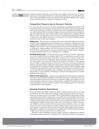
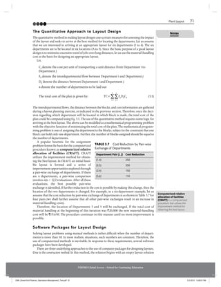
Consider a job shop with five machines and four jobs. Each
job has a processing sequence in which it visits three out of
the five machines. Each job also has a due date for comple-
tion. The relevant information is given in Table 8.9.
(a) Use SPT and EED rules to obtain the schedules for
the jobs.
(b) Compute the make span, mean lateness and num-
ber of tardy jobs.
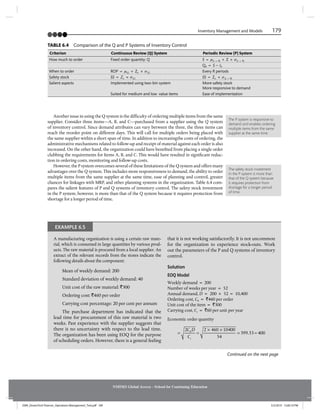
Solution
We use a Gantt chart to develop the schedule for the shop.
SPT Rule:
Jobs 2 and 4 require processing in Machine 1. However,
since the processing time of Job 4 is less than for Job 1 it
is scheduled first in the machine using SPT. Similarly, Job
1 is first scheduled in Machine 2. The partial Gantt chart is
shown in Figure 8.5.
At the end of time unit 3, Job 1 exits Machine 2 and it
is time to take the next scheduling decision. Job 1 will be
scheduled in Machine 4 as there is no other job compet-
ing for that machine. Similarly Job 3 will be scheduled in
Machine 2. The Gantt chart in Figure 8.6 has these addi-
tional schedules included.
EXAMPLE 8.4
Machine 5
Machine 4
Machine 3
Machine 2
Machine 1
1 1 1
4 4 4 4 4
1 2 3 4 5 6 7 8 9 10 11 12 13 14 15 16 17 18 19 20 21 22 23
FIGURE 8.5 The partial Gantt chart for the SPT rule
TABLE 8.9 Details for each Job
Processing Time (Machine
Visited in the Sequence)*
Jobs 1 2 3 Due by
Job 1 3 (2) 7 (4) 3 (5) 10
Job 2 6 (1) 3 (2) 7 (5) 12
Job 3 7 (2) 3 (4) 4 (3) 9
Job 4 5 (1) 4 (3) 5 (4) 14
Note: *The numbers in the parenthesis indicates the machine in
which the job gets processed
8.6 SCHEDULING OF JOB SHOPS
As we have already noticed, scheduling is much more complicated in the case of a job shop.
Unlike the flow shop, developing optimal methods is difficult and computationally complex.
Complete enumeration is also not possible as the number of schedules [(n!)m
] grows exponen-
tially with n and m. Therefore, the use of appropriate scheduling rules and performance criteria
are the only viable options for the planner. Use of graphical methods such as Gantt charts is very
useful for job-shop scheduling. However, unlike the case of flow shops, the performance of vari-
ous scheduling rules cannot be easily predicted in a job shop. Therefore, one can resort to simu-
lation modelling of the system and evaluate alternative scheduling rules.
The use of graphical
methods such as Gantt
charts is very useful for job-
shop scheduling.

Machine 5
Machine 4
Machine 3
Machine 2
Machine 1
1 1 1
4 4 4 4 4
1 2 3 4 5 6 7 8 9 10 11 12 13 14 15 16 17 18 19 20 21 22 23
3 3 3 3 3 3 3
1 1 1 1 1 1 1
FIGURE 8.6 The Gantt chart with the additional schedules
Machine 5
Machine 4
Machine 3
Machine 2
Machine 1
1 1 1
4 4 4 4 4
1 2 3 4 5 6 7 8 9 10 11 12 13 14 15 16 17 18 19 20 21
3 3 3 3 3 3 3
1 1 1 1 1 1 1
2 2 2 2 2 2
2 2 2
4 4 4 4 3 3 3 3
1 1 1
3 3 3 4 4 4 4 4
2 2 2 2 2 2 2
FIGURE 8.7 The ﬁnal Gantt chart for the SPT rule
Machine 5
Machine 4
Machine 3
Machine 2
Machine 1
1 2 3 4 5 6 7 8 9 10 11 12 13 14 15 16 17 18 19 20 21 22 23
3 3 3 3 3 3 3
2 2 2 2 2 2
2 2 2
3 3 3 3
3 3 3
1 1 1
2 2 2 2 2 2 2
4 4 4 4 4
1 1 1 1 1 1 1
4 4 4 4
1 1 1
4 4 4 4 4
FIGURE 8.8 The Gantt chart for the EDD schedule

242 Chapter 8
8.7 INPUT–OUTPUT CONTROL
Operational control in manufacturing systems is largely a function of the relationship between
input and output rates. Let us look at a situation in which jobs are launched into system at the
rate of one every four hours and the jobs leave the system one every three hours. Over a period of
time one could expect build-up of inventory in the system leading
to congestion at workstations and chaos in material flow. Build-up
of WIP inventory in the system leads to several complications,
which include the following:
(a) Estimating the available capacity in the shop becomes difficult.
(b) The lead time for manufacturing increases with increase in
inventory.
(c) Planning and control of operations becomes more complex as
more jobs compete for limited resources.
(d) Performing loading and scheduling functions also becomes
difficult.
Therefore, input–output control is an important element of
operational control in manufacturing systems, especially in batch
manufacturing and job-shop systems. Figure 8.9 portrays the input–
output control mechanism required for a manufacturing system
with the analogy of a water-flow system that has a pair of control
gates. The first control is at the input of pending orders into the sys-
tem and the second control point is the output rate. By a judicious
choice of the input and output rates, better planning and control can
be achieved and lead times reduced to realistic levels. The basis on
which the two control points will be adjusted is the quantum of con-
stant WIP (CONWIP) in the system.
8.8 OPERATIONAL CONTROL ISSUES IN MASS PRODUCTION
SYSTEMS
So far, we have concentrated on flow shops and job shops and issues pertaining to scheduling and
operational control in these systems. However, there are several examples of mass production
systems in operation today. For example, a two-wheeler manufacturer such as Bajaj Industries
One can proceed in this fashion to arrive at the
final chart for the SPT rule, as shown in Figure 8.7. It
may be noted that the SPT rule is invoked only when
more than one job competes for a resource. The make
span for the problem is 21 units as evident from the
Gantt chart.
The EDD rule schedule is drawn using a similar logic.
When there are competing jobs for a resource, the EDD
criterion is used. The Gantt chart for the EDD schedule is
given in Figure 8.8.
In this case, the make span has increased by two time
units to 23. Table 8.10 presents a summary of the perfor-
mance measures for SPT and EDD rules. Interestingly,
the EDD rule has fared badly on completion time, make
span and lateness. This example clearly demonstrates the
complexity of job shops. Predicting the performance of the
rules is not as easy as in the case of a flow shop. In both the
cases, all the jobs were tardy.
TABLE 8.10 Performance Measures for SPT and
EDD Rules: A Summary
Job
Number
SPT EDD
Due Ci Lateness Ci Lateness
1 10 13 3 23 13
2 12 21 9 20 8
3 9 17 8 14 5
4 14 18 4 23 9
Average 17.25 6.00 20.00 8.75
Pending
orders
Input rate
control
Existing
load
Completed
orders
Output rate
control
CONWIP
FIGURE 8.9 Input–output control: an illustration

produces over 9,000 two wheelers everyday. Various sub-assemblies in the Bajaj plant need to be
configured to match the production rate. Similarly, the final assembly stations should also have
the required number of resources at each station to meet the targeted demand. In such a scenario,
much of control and scheduling boils down to appropriately arriving at a balanced flow of com-
ponents on the shop floor. There are two ways of achieving this objective:
(a) Estimate the number of resources required at each station of the manufacturing system for
a targeted production level. Conversely, if there are a certain number of resources available,
estimate the production level and adjust the plans accordingly.
(b) Given a certain availability of resources at various stages of the production system and a tar-
geted daily production, estimate the rate at which the entire system should work and accord-
ingly modify the work practices and resource deployment to meet the target.
The first method lays emphasis on designing operational control systems for mass produc-
tion. On the other hand, the second method focuses on the ability to craft alternative operational
control strategies to meet the changing targets on a period-to-period basis. The former is a tra-
ditional application of the concept and is often referred to as the line-balancing technique, while the
latter is the modern Japanese approach to manage mass production systems. A detailed descrip-
tion of line balancing is available in Chapter 4 of the book.
The line-balancing technique does not solve all the operational control problems in a mass
production system. It provides a basis for the initial design and deployment of resources.
However, mass production systems face constant revisions in the production rate. These changes
occur due to changes in the market demand and revisions in component off-take by custom-
ers. Consider an auto-component manufacturing firm, such as the Chennai-based Lucas TVS
that supplies alternators to Maruti Udyog Limited (MUL). Suppose the daily requirement of
MUL is 480 alternators during the first week of a month. If Lucas works for two shifts of eight
hours each, then the hourly production of alternators is 480/16 = 30. Furthermore, the cycle
time for alternator assembly is 60/30 = 2 minutes. This means that the production system
responsible for manufacturing alternators for MUL should work at a uniform pace with a cycle
time of two minutes everywhere. The final assembly will have to be tuned to two minutes, and so
will all the feeder shops to the final assembly.
Suppose that there has been a revision in the daily requirement by the third week of the month.
Due to increased production at their plant, let us assume that MUL wants a daily supply of 600
alternators. To cope up with the increase in the demand, Lucas will have to work with a new cycle
time 20 per cent less than the earlier measure (that is, 1.6 minutes). The final assembly as well as all
the feeder units will have to be tuned to this new requirement. This measure therefore provides a
rhythmfortheoverallfunctioningoftheshop.Inmassproductionsystems,thismeasureisknown
as TAKT time. Operational control issues in mass production systems begin with the computation
of TAKT time. Based on this, several choices are made to ensure that the actual cycle time is as per
the computation of TAKT. These choices can be grouped under the following categories: machine
redeployment, altering operator allocations, and adjusting material feed rates.
Operational control issues in
mass production systems begin
with the computation of
TAKT time.
TABLE 8.11 An Illustration of Worker Deployment for Adjusted TAKT Time
Required output per day 400 450 371
Number of shifts per day 2 2 2
Required output per shift 200 225 185.5
Net available production time (minutes) 420 420 420
TAKT time (seconds) 126 112 136
Work content (seconds) 1,764 1,764 1,764
Number of operators required per shift 14 16 13
Total number of operators required 28 32 26
Notes
Notes

244 Chapter 8
Machine Redeployment
Mass production systems lay emphasis on the flexibility of the varying deployment of resources
to alternative product groups. Therefore, one method of responding to changing TAKT time is to
alter the assignment of machines (or manufacturing cells) to specific product groups. By incre-
mental addition/deletion of machines, it is possible to adjust the production rate and cycle time.
Altering Operator Allocations
Operators in a mass production system are often expected to be multi-skilled. Therefore, one way
of adjusting the cycle time is to alter the worker allocations. If a worker was attending to three
machines earlier, then by adding additional workers to the manufacturing cell, the cycle time can
be reduced, and vice versa. Such practices are common in mass production systems. Table 8.11
presents an illustrative example of this. In this example, for a required daily output of 400 units,
the output required per shift is 200 units. Since the net available production time is 420 minutes,
the TAKT time comes to 126 seconds. When the daily output is increased from 400 to 450, it
required adjustment of the TAKT time from 126 seconds to 112 seconds in order to continue
working on a two-shift basis. However, the number of workers has increased from 28 to 32 (2
additional workers per shift). Typically, employees will be deployed from another product line to
this one to meet the new daily requirement. On the other hand when the daily output falls to 371,
two workers need to be taken out of the production line (one per shift) and redeployed elsewhere.
Adjusting Material Feed Rates
Mass production systems have a streamlined material flow, often achieved by installing a conveyor
system. The speed at which the conveyor moves between stations is a function of the cycle time. For
instance, if two stations are five metres apart and the TAKT time is 30 seconds, then the conveyor
needs to move between stations at a speed of 1 metre every 6 seconds (10 metres per minute). On
the other hand, if the TAKT time changes to 20 seconds, the conveyor speed should be adjusted to
1 metre every 4 seconds (15 metres per minute). Furthermore, the tasks to be completed at every
workstation needs to be completed within 20 seconds.
8.9 OPERATIONS PLANNING AND CONTROL BASED ON THE THEORY
OF CONSTRAINTS
In this chapter, we have discussed various techniques for scheduling operations in a job shop and
a flow shop. However, despite the use of these, there is a common problem of high WIP inventory
in several manufacturing organizations. Moreover, manufacturing organizations suffer from
the “end-of-the-period” syndrome. Typically, as organizations approach the end of a reporting
period (the year-end is a classic example, but there are monthly and quarterly reporting cycles
also), workflow gets considerably complex and inventory piles up beyond normal limits. Several
reasons are attributed to this and significant among them are the following:
(a) Organizations do not use appropriate measures for performance.
(b) Operations scheduling does not take into consideration some ground realities in the shop
floor.
Measures based on standard costing, such as variances at the department or even work-centre
level, promote local optimum at the expense of global optima. Therefore, it is possible to create
mountains of inventory, yet products may not flow evenly out of the manufacturing system.
Similarly, scheduling on the basis of balancing capacity at individual work-centre level may not
ensure a smooth flow of material through the manufacturing system.
Measures of Performance
The theory of constraints developed by Eliyahu Goldratt addresses these concerns and pro-
poses alternative methodologies for operations scheduling. Goldratt also proposed three new
measures of performance for manufacturing firms.
Notes

➱ Operational measures: The operational measures for a company are the throughput, inventory,
and operational expenses. These measures could be used to make all decisions pertaining to
the use of manufacturing resources.
➱ Throughput: Throughput is the quantity of money generated by a firm through sales over a
period of time. The standard definition of throughput is total output, but this definition con-
siders only sales and not finished goods (FG). According to Goldratt, this is because finished
googs do not generate revenue for the firm until they are sold.
➱ Inventory: The quantity of money invested in materials that a firm intends to sell is defined as
inventory. Contrary to the traditional logic (where inventory valuation includes value-added
components to estimate WIP and FG inventory), here, it is a simple measure of the value of
the material only.
➱ Operating expenses: Operating expenses include all expenses incurred by a firm to convert
inventory into throughput over a period of time.
According to the theory of constraints, it is possible to increase the throughput even while the
operating expenses and inventory are being reduced. This is identified as the single most impor-
tant goal of managing manufacturing organizations. The principles governing the theory of con-
straints are best explained using the analogy of marching soldiers.
The Analogy of Marching Soldiers
The problems associated with scheduling and operational control of manufacturing systems can
be best explained using the analogy of a column of marching soldiers. Assume that a batch of 10
soldiers begin the march from a reference point. Initially, all the 10 soldiers will be one behind
the other with an equal gap. However, as they begin to march, certain differences will be noticed.
If we observe the marching soldiers, we may find that the distance between the first and the last
soldier is more than what it was at the starting position. This is because as the soldiers engage in
marching, differences in the speeds and capacities of each soldier begin to manifest. If the third
soldier is slower than the first two, then the gap between the third and the other two soldiers
ahead of him will increase with time. If we observe the marching soldiers after they have covered,
say, 5km, the gap will increase even further.
Scheduling and operational control problems in manufacturing organizations share con-
siderable similarity with this analogy of marching soldiers. The ground to be covered in the
marching-soldiers example is the same as the raw material in the case of manufacturing organi-
zations, and the ground already covered corresponds to finished goods. On the other hand, the
mounting gap between the first and the last soldier is equivalent to the work-in-process inven-
tory in a manufacturing organization (see Figure 8.10 and Table 8.12 for a graphical representa-
tion of this).
As in the case of the soldiers, resources in manufacturing organizations differ from one
another in their ability to process components. Some machines may have more than the required
According to the theory of
constraints, it is possible
to increase the throughput
even while the operating
expenses and inventory are
being reduced.
Raw material
Marching soldiers
Finished goods
Work in process
FIGURE 8.10 Marching soldiers: an analogy for planning and control in
manufacturing systems
Notes

246 Chapter 8
capacity to process in a planning horizon. Some other resources may have less than the total
capacity required for the planning horizon. Statistical fluctuations and dependent events are
characteristic of resources in a manufacturing organization. All these generate similar effects in a
manufacturing system as that of increasing the gap between the soldiers. However, we know that
increasing WIP inventory and manufacturing lead time is directly related to the increase in the
gap between the soldiers as they march. Therefore, operational control is primarily a function of
making sure that the gap between the soldiers does not increase with time.
The theory of constraints is a systematic body of knowledge that recognizes these effects in a man-
ufacturing system and uses specific methods to improve the performance of the system under
these conditions. Synchronous manufacturing is a specific application of the theory of con-
straints to scheduling and operational control of the manufacturing systems.
Synchronous Manufacturing
The marching-soldiers example shows that the rate at which they can cover ground is a function
of the slowest marching soldier in the column. If soldiers ahead of the slowest continue to march
at their higher speeds, they will only contribute to increasing the gap between them and the slow-
est. On the other hand, those behind the slowest will be forced to march only at the speed of the
lowest. One way to solve this problem is to first tie a rope connecting all the soldiers (from the
first to the last), and provide a drumbeat at a rate equivalent to the slowest and enable the march-
ing soldiers to respond to the rhythm of the drumbeat. By doing this we not only ensure that the
gap does not increase with time, but also create a synchronized movement of the soldiers on the
ground. Synchronous manufacturing deploys these features in the scheduling and operational
control logic. In synchronous manufacturing, the focus is on synchronizing flow rather than on
balancing capacities.
This discussion clearly brings out the need to address the scheduling problem in a different
context. It is important to plan the scheduling and control of the entire manufacturing system
on the basis of availability of resources. The following definitions are common in synchronous
manufacturing literature.
➱ Bottleneck resource: Any resource whose capacity is equal to or less than the demand placed on
it is a bottleneck resource. On the contrary, any resource whose capacity is more than the
demand placed on it is a non-bottleneck resource.
➱ Capacity constrained resource (CCR): In a manufacturing system it is observed that some
resources have the ability to significantly deviate the product flow, from the planned flow, if
not properly scheduled. Any resource that can deviate the actual product flow from the
planned flow is known as a capacity constrained resource. A bottleneck or a non-
bottleneck resource may become a CCR.
➱ Activation of a resource: Activation merely refers to the deployment of a manufacturing
resource to process materials. Merely processing material may not in itself guarantee
increase in throughput.
➱ Utilization of a resource: Utilization refers to the activation of a manufacturing resource that
will lead to improving the throughput.
Synchronous
manufacturing is a specific
application of the theory of
constraints to scheduling
and operational control of
manufacturing systems.
Any resource whose
capacity is equal to or less
than the demand placed
on it is a bottleneck
resource.
Any resource that can
deviate the actual product
flow from the planned flow
is known as a capacity
constrained resource
(CCR).
TABLE 8.12 A Comparison of Marching Soldiers and a Production System
Resource Marching Soldiers Production System
Processing Ground to be covered Raw material to be processed
WIP Gap between the ﬁrst and the last soldier Work in process in the shop ﬂoor
Throughput The extent of ground covered by the marching
soldiers
Amount produced and sold by the
production system
Operating expenses Amount of energy expounded by the soldiers to
complete the march
Cost of transforming the raw material into
throughput
Objective To cover a certain extent of the ground in a given
time
To achieve a certain throughput in a given
time

➱ Process batch: A process batch refers to the quantity of a product (or part) processed at a
resource before that resource changes over to another product (or part). For example, if two
parts—X and Y—are processed in Resource R1, then, if 300 units of Part X are processed
before changing over to processing Part Y, then the process batch for Part X is 300.
➱ Transfer batch: A transfer batch indicates the quantity moved at the same time from one
resource to another resource in a manufacturing system. For example, if 100 units of Part
X are moved at a time from Resource R1 to Resource R2 for further processing, then the
transfer batch of Part X is 100.
Constraints in a Manufacturing System
Before we address the issue of scheduling with bottleneck resources as the focus, it is helpful to
understand how bottlenecks develop in an organization. In a broad sense, bottlenecks are noth-
ing but the manifestation of constraints. In synchronous manufacturing, any element that pre-
vents the system from increasing its throughput is identified as a constraint. There are several
constraints in an organization—some of them are hard constraints and others soft. By hard, we
mean constraints arising out of capacities, physical infrastructure, resource availability, and so on.
On the other hand, soft constraints arise out of policy implications and poor managerial practices.
For example, a peculiar and complicated approval process for purchase order release may result in
severe material constraints (due to long lead time for procurement). Soft constraints are not obvi-
ous to the management. They manifest indirectly in other forms of hard constraints (as our pur-
chase order example shows). It requires special attention to track and remove those constraints.
Market constraints are the limits of production imposed by the market demand. Capacity
and material constraints arise out of physical limitations in capacity and material availability.
For instance, the short supply of a key ingredient in a manufacturing process puts limits on the
system. Similarly, the capacity of available machines and human resources may impose limits
on the system. There are also soft constraints arising out of managerial, logistical, and behav-
ioural issues.
Synchronous manufacturing may offer valuable help in scheduling a manufacturing system
with constraints. However, in the long run, it is important to invest in methods to remove the
constraints. Removing an existing constraint merely shifts the constraint elsewhere and is there-
fore an ongoing process, as indicated in Figure 8.11.
The guiding principles of synchronous manufacturing are as follows:
1. Do not focus on balancing capacities. Instead, focus on synchronizing the flow.
2. The marginal value of time spent at a non-bottleneck resource is negligible. Do not attempt
to reduce time at a non-bottleneck resource.
2a. An hour gained at a non-bottleneck resource is a mirage.
2b. An hour lost at a non-bottleneck resource is an hour of throughput loss.
Soft constraints
Hard constraints
Constraints shift elsewhere
Mount a time-bound procedure
for removing the constraint
Gainfully exploit it using
synchronous manufacturing
Identify the constraint
Progressive mindset
Process improvements
Revised systems
FIGURE 8.11 Constraint management in the long run
Notes

248 Chapter 8
3. The level of utilization of a non-bottleneck resource is controlled by other constraints within
the system
4. Resources in the system must be utilized, not simply activated.
5. A constraint is any element that prevents the system from achieving the goal of making
more money.
6. The transfer batch need not, and many times should not, be equal to the process batch
From the definitions and the guiding principles we have discussed, a few important aspects can
be inferred:
➱ The separation of resources as bottleneck and non-bottleneck is very important because
while bottleneck resources determine the (planned) output of the system, CCR will ensure
that the actual throughput does not deviate from the plan in a manufacturing system. Focus-
ing on maximizing the utilization of a bottleneck resource is instrumental to maximizing the
throughput in a manufacturing system. On the other hand, scheduling is done in synchro-
nous manufacturing with reference to CCRs.
➱ Placing buffers in front of bottleneck resources will protect the throughput of the system
➱ Careful choice of the transfer and process batch sizes will ensure the protection of the
throughput at the bottleneck as well as proper scheduling of the CCRs
➱ Once these aspects are determined, the rest of the system must work in tandem with these
decisions
A drum–buffer–rope (DBR) methodology helps one to achieve these while scheduling a manu-
facturing system.
The Drum–Buffer–Rope (DBR) Methodology
Once a preliminary production plan is established, synchronous manufacturing develops
detailed schedules for the CCRs in the plant. On the basis of these schedules, the production
plan can be finalized. The resulting modified production plan can become the master production
schedule (MPS) and can be used as the basis for making promises to customers. This process of
arriving at the MPS on the basis of the detailed schedules for CCRs is the drum in DBR methodol-
ogy. The MPS, which is based on the processing capabilities and requirements of the CCRs, deter-
mines the pace and the sequence of production for the entire plant. The MPS itself is therefore
analogous to the drumbeat of the march. The drumbeat ensures that all resources are not merely
activated but utilized as per the throughput requirement.
Since statistical fluctuations are inevitable, there could be potential opportunities for the
planned flow to deviate from the actual flow. To protect the schedule from disruptions, a time
buffer is built into the system. The planned lead time is the sum of the process and set-up times
andthetimebuffer.Ineffect,thetimebufferincreasestheplannedleadtimebyasufficientamount
so as to accommodate disruptions and fluctuations that are likely to happen in the manufacturing
system. Since the bottleneck resource dictates the output of the entire system, an hour of capacity
lost at the bottleneck translates directly into an hour of lost throughput. Therefore, the buffer is
placed in front of a bottleneck resource. On the contrary, nothing is achieved by placing a buffer
ahead of a non-bottleneck resource. It merely increases the inventory in the system but not the
throughput.
Once the MPS is finalized, the product structure, routing sheets, and other production pol-
icies are used to determine the quantity and timing of planned production at each resource
in the plant. Since the MPS is based on the capabilities of CCRs, the entire plant operation is
tied through this process to the drumbeat of the MPS. Through this methodology, we have
ensured synchronization of schedules at all non-CCRs. Therefore, this is the rope component
of the DBR methodology. Figure 8.12 illustrates the DBR methodology in the case of a bot-
tleneck resource in a shop having seven resources. The DBR methodology can be outlined as
follows:
(a) Develop the MPS so that it is consistent with the constraints of the systems (Drum).
(b) Protect the throughput of the system from statistical fluctuations through the use of buffers
at some critical points in the system (Buffer).
(c) Tie the production at each resource to the drumbeat (Rope).
Notes

Several organizations have benefited from the use of the DBR methodology for scheduling
operations in a manufacturing system. In response to the demand for easy application of these
principles, several computer-based software packages have also been developed to implement
the DBR methodology. Synchronous manufacturing principles represent a recent approach to
addressing scheduling complexities in organizations. Moreover, the notion of the theory of con-
straints is also applicable to other operations systems such as management of large projects.
Communication (Rope)
Buffer
Bottleneck (Drum)
A B C D E F G
FIGURE 8.12 An illustration of the DBR methodology
• The focus shifts from operations planning to operational
control in the short term. Scheduling aids operational
control in manufacturing and service systems.
• The scheduling context relates to the number of jobs and
machines in the system and the physical configuration of
the machines. These factors greatly influence the com-
plexity of scheduling.
• Flow shops and job shops are two alternatives for the
configuration of a manufacturing system. The schedul-
ing methodology and complexity differ vastly between
these two. Job shops are far more complex to schedule
than flow shops.
• Johnson’s algorithm provides an optimal schedule
for a two machine–n job problem using the shortest
processing time rule for scheduling. Several variations
of Johnson’s algorithms are available for flow-shop
scheduling.
• Operational control in mass production systems are
primarily achieved through use of TAKT time–based
scheduling.
• The theory of constraints indicates that schedul-
ing of operations must take into account the exist-
ence of bottlenecks and statistical fluctuations in
operations.
• Synchronous manufacturing principles apply the theory
of constraints and develop alternative schedules using a
drum–buffer–rope methodology.
S U M M A R Y
1. Critical Ratio
Remaining time
Remaining work
Due date
( )
(
=
=
−Current dat
C
C e
Remaining processing time
)
2. Flow time of the job, Fi i
F
F i
( )
R C
i
R i
−
Ri
R
3. Make span (maximum completion time), C C
i
i
max x{ }
4. Lateness of the job, Li i i
( )
C D
i
C i
−
Ci
C
5. Tardiness of the job, Ti i
T
T ( , )
Li
L
0
R
R V
O E
M I
U E
L A W
F
1. How is scheduling linked to other aspects of production
planning? Explain with the help of an example.
2. What do you mean by the loading of machines? What do
you achieve by performing the loading function?
3. Classify the following as a job shop or as a flow shop for
the purpose of scheduling. Also, identify the relevant
parameters of the system that have a bearing on the
scheduling complexity.
(a) Executive health check-up in a hospital
(b) Tirupati temple queue complex having multiple
stages
(c) Breakfast buffet system at Taj Hotel
Q
R V
E U
I E
E S
W T I O N S
Notes

250 Chapter 8
M
P O
R S
B L E
1. Consider a one-machine–six-jobs scheduling prob-
lem. All the jobs are available for scheduling at the
beginning of the planning horizon itself. The pro-
cessing times and due dates of the jobs are given in
Table 8.13.
(a) Use LPT, SPT, FCFS, RAN, EDD, and SR to arrive at a
schedule
(b) For each of the schedules, compute the following
performance measures:
i. Mean flow time
ii. Make span
iii. Mean completion time
iv. Mean lateness
v. Mean tardiness
vi. Number of tardy jobs
(c) Identify the rule that performs the best for each of
these performance criteria.
2. A service provider has two stages in service delivery.
Initially, the customers arrive at Stage 1, get the initial
part of the service, and then reach Stage 2, where the
remaining part of the service is completed. All arriv-
ing customers wait in a lounge and are called on some
basis into the system once a batch of eight accumulates.
All of them go through these two stages, although the
time they spend in these two stages may vary depend-
ing on their specific requirements. The time spent by a
set of eight customers on these two stages is shown in
Table 8.14.
(a) Use Johnson’s rule to schedule customers in the
system.
(b) Develop a Gantt chart for the schedule.
(c) Identify key performance measures for this situation
and compute them for the solution obtained using
Johnson’s rule.
(d) If you scheduled the customers using FCFS, what is
its impact on the performance criteria?
TABLE 8.13 Processing Times and Dates of Jobs
Job 1 Job 2 Job 3 Job 4 Job 5 Job 6
Processing
time (minutes)
12 10 15 13 12 9
Due (minutes
from start
of planning
horizon)
25 45 55 30 90 70
(d) Final assembly shop of a computer manufacturer
(e) Computerized passenger reservation system of
Indian Railways
(f) Eye camps conducted by a local eye hospital
(g) A common heat treatment facility in a
manufacturing plant
(h) Visa section at the US consulate office at Mumbai
4. How would you determine the complexity of the sched-
uling problem?
5. A firm is interested in choosing between the minimiza-
tion of make span and minimization of flow time as the
performance criterion. Prepare a short note advising
them on the pros and cons of using these rules.
6. What are the implications of using completion-based
measures as opposed to due date–based measures for
evaluating scheduling rules?
7. Explain, by means of a simple example, the difference
between lateness and tardiness. Which is a better meas-
ure? Why?
8. What is a Gantt chart? What is its use in scheduling?
9. What is cycle time? What are the practical implications of
cycle time measure in mass production scenarios? How
do they influence the scheduling of jobs in a manufac-
turing system?
10. An organization has a certain number of worksta-
tions in its final assembly for a desired production
rate. If the desired production rate has gone up by
10 per cent, how would you respond to the new
requirement? Will this change have an effect on cycle
time?
11. What do you mean by soft and hard constraints in an
organization?
12. How are synchronous manufacturing principles differ-
ent from the traditional methods used for scheduling of
jobs?
13. What is meant by the DBR methodology? What does it
seek to achieve?

(e) Evaluate and compare the performance of the random
rule with Johnson’s rule and the FCFS rule.
3. A pure flow shop has three machines and all the jobs visit
these machines. The processing time of each job in each
machine is given in Table 8.15.
(a) Use the SPT rule to schedule the jobs in the flow shop
and draw a Gantt chart for the schedule.
(b) Compare the performance of the SPT rule
with the EDD rule using the following performance
criteria:
i. Mean tardiness
ii. Mean flow time
iii. Number of tardy jobs
iv. Make span
(c) Compute the utilization of the three machines for
both the schedules.
(Hint: Convert it into a two machine problem.
First alternative is to combine processing times of
m/c1 and m/c2 into a single equivalent machine.
Alternative 2 is to combine the processing times m/
c2 and m/c3. Solve using Johnsons rule and choose
the best alternative)
4. A job shop has five machines for processing. There are
six jobs to be processed. However, current capacity con-
straints indicate that only five jobs can be processed
out of the six. The planner needs to know which jobs to
assign to the machines. Identify an optimal loading of the
shop on the basis of Table 8.16, which contains data on
the processing time of each job against each machine.
5. A job shop has five jobs for processing. There are four
machines in the shop. The jobs visit the machines in a
particular order (indicated by each job’s routing file).
Table 8.17 has details of the machines visited by each job
and the processing time of each machine. The table also
has information on the due dates.
(a) Develop a schedule for the jobs using (i) SPT, (ii) EDD,
and (iii) FCFS rules.
(b) Use three appropriate performance criteria and
evaluate these rules.
(c) Compute the machine waiting time and job waiting
time for all the schedules obtained using the SPT, EDD
and FCFS rules. If you were to select a scheduling rule
on the basis of the minimum job waiting time, what
will your recommendation be?
(d) If there is a penalty for delay at the rate of `250
per minute and a reward of `100 per minute for
completing early, compute the cost of the schedules
attributable to these.
TABLE 8.15 Processing Time of Jobs, Machine-wise
Job Number
Processing Time 1 2 3 4 5 6 7 8
Machine 1 (minutes) 14 10 10 13 12 11 9 9
Machine 2 (minutes) 11 14 10 9 14 14 7 10
Machine 3 (minutes) 9 8 10 11 12 7 8 9
Due (minutes from
start of planning
horizon)
80 45 55 60 90 50 100 70
TABLE 8.16 Processing Time of Jobs
Machines
Jobs A B C D E
1 11 14 17 10 12
2 12 14 16 13 10
3 17 12 11 15 12
4 16 16 12 12 14
5 14 16 10 11 12
6 15 14 13 16 19
TABLE 8.14 Duration Spent by Customers on
the Two Stages
Customer Number
1 2 3 4 5 6 7 8
Stage 1
(minutes)
11 10 9 13 12 10 9 11
Stage 2
(minutes)
9 14 10 12 14 14 11 10
Arrival time
(minutes from
start of batch)
0 1 3 4 5 7 8 10
TABLE 8.17 Processing Time of Jobs and Due
Dates
Machines Visited (Processing Time In Minutes)
Jobs 1 2 3 4 Due by (minute)
1 1 (12) 3 (7) 4 (8) 5 (4) 45
2 2 (7) 4 (6) 3 (5) 5 (6) 35
3 1 (8) 2 (5) 3 (9) 4 (5) 37
4 3 (6) 1 (6) 2 (6) 5 (7) 29
5 2 (9) 4 (8) 5 (6) 3 (7) 40

252 Chapter 8
1. A vast number of scheduling packages are avail-
able in the market today. Scan through the following
sources:
• Journals: OR/MS Today (a bimonthly magazine from
the Operations Research Society) and IIE Solutions (a
journal of the Institute of Industrial Engineering). These
journals periodically bring out a survey of available
software for specific areas of production management.
Look for surveys pertaining to scheduling software.
• American Production & Inventory Control Society
(APICS).
• Search engines: Search with keywords such as “APS”,
“advanced production scheduling”, and “scheduling
software”.
(a) Based on this exercise, prepare a technical note
on a survey of the available software options for
scheduling.
(b) Develop a classification scheme to list all the soft-
ware that you have come across.
2. Visit a health management system (such as a multi-spe-
cialty hospital with facilities for in-patients, out-patients,
laboratories for diagnostics, operation theatres, and spe-
cial care systems) and study the scheduling practices with
respect to the following:
• The doctors and surgeons visiting the hospital
• The support staff such as nurses, shift doctors, co-
workers and laboratory staff
• Major facilities such as operation theatres and
laboratories
• The outpatient department
(a) Prepare a note outlining the major findings of
the study with respect to the aspects mentioned
here. The report should highlight the relevance of
scheduling techniques discussed in the chapter,
the extent of usage, reasons for non-usage, and
recommendations for removing some of the bar-
riers to adopting the known techniques.
(b) Did you notice any significant patterns in the
scheduling of personnel in the system that differs
from a typical manufacturing system?
(c) If so, identify them and state the reasons for the
differences.
3. Read the book The Goal by Goldratt and Cox. After read-
ing the book, write a book review. While writing the
review, answer the following questions amongst other
things that you may like to cover in the book review:
(a) What are the key elements of the alternative method
by which Alex Rego tries to solve the problems at
his manufacturing set-up? Clearly outline the key
conceptual details of his alternative strategy that
helped him find a solution.
(b) How do you link his strategies for controlling a
manufacturing system to that of the notion of
scheduling that we have discussed in the chapter?
(c) What are the key performance measures that
Alex Rego uses for controlling his manufacturing
system?
(d) Doyouthinkthathisconcepthasawideapplicability?
If so, give some examples of situations where this
concept can be applied.
R
N J
I O
I E C
P T
M S
6. A bulb manufacturer works for 25 days a month on a two-
shift basis. Each shift is of 8 hours duration. The marketing
demand estimates the monthly demand for the bulbs to
be 48,000. If the manufacturing system is a continuous-
flow mass-manufacturing type with feeder shops linked
to the assembly shops through a material flow control
system, then compute the following for the manufacturer:
(a) The TAKT time for all the shops in the manufacturing
system.
(b) If the successive workstations in the manufacturing
plant are uniformly placed at a distance of three
metres, at what speed should the material handling
system move between the work-stations?
Notes

Answer Keys: 8-1. D 8-2. D 8-3. C 8-4. A 8-5. D 8-6. A 8-7. B 8-8. D 8-9. D 8-10. A
8-1. What system uses a defined framework to address
issues associated with the use of available resources
and the delivery of products and services as prom-
ised to the customers?
A. MRP system
B. Procurement Scheduling
C. Production Scheduling
D. Operations Scheduling
8-2. Which is the process of rank-ordering the jobs in
front of each resource to maximize some chosen
performance measure?
A. Loading
B. Scheduling
C. Routing
D. Dispatching
8-3. What is the useful method when one job is assigned
to one machine and there are as many machines
available for assignment a there are jobs?
A. Process Planning
B. Flexible Manufacturing Systems
C. The Assignment Method
D. Production Planning
8-4. What are the parameters adequately describe the
scheduling problems that one tries to solve?
A. Number of machines, Number of jobs, Shop
configuration
B. Processing time, Due date, Random order
C. Completion measure, Inventory, Cost
D. Due date measure, Lateness, Work-in-Progress
8-5. With how many sets of jobs possible, the floor shop
becomes a shop?
A. One
B. Two
C. Three
D. Four
8-6. For Job-shop scheduling which is the very useful
graphical method?
A. Gantt charts
B. SPT rules
C. EED rules
D. Operating system
8-7. What is an important element of operational control
in manufacturing systems, especially in batch manu-
facturing and job-shop systems?
A. Production control
B. Input-Output control
C. Time control
D. Operation control
8-8. Operational control issues in mass production sys-
tems begin with the computation of:
A. Initial Environment Review (IER)
B. Environment Management System (EMS)
C. Health, Safety and Environment (HSE)
D. TAKT time
8-9. What was developed by Eliyahu Goldratt?
A. The Analogy
B. Synchronous
C. Bottleneck resource
D. The theory of constraints
8-10. Which is the administrative process of authorizing
processing of jobs?
A. Dispatching
B. Receiving
C. Allocating
D. Distributing
Notes

Notes

Operations-Management.pdf

More Related Content

What's hot

Similar to Operations-Management.pdf

Recently uploaded

Operations-Management.pdf