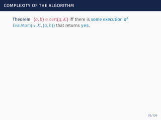
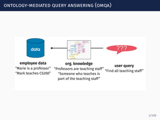
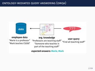
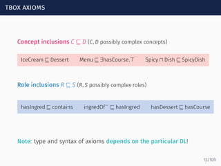
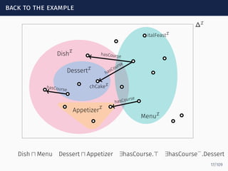
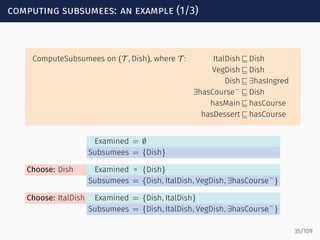
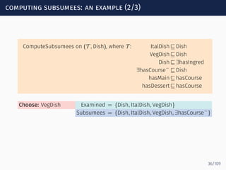
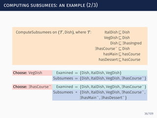
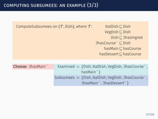
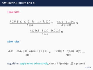
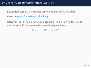
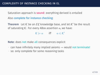
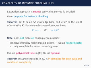
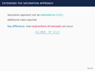
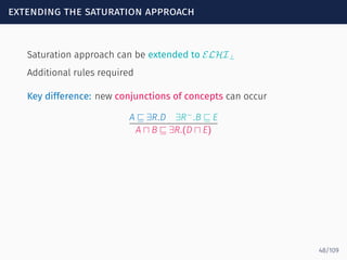
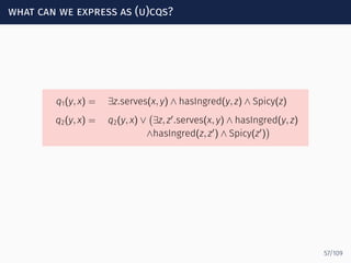
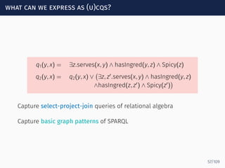
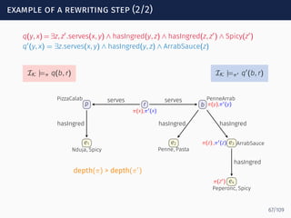
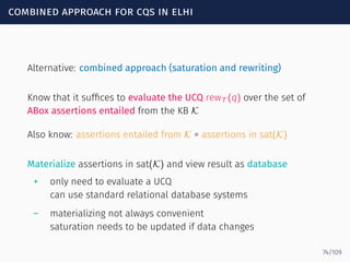
The document discusses ontology-mediated query answering (OMQA) using description logics, focusing on applications in medicine, life sciences, and enterprise information systems. It highlights the benefits of ontologies in standardizing terminology, enhancing data integration, and supporting automated reasoning. The tutorial covers the fundamentals of Horn description logics and their implications for effective query answering.


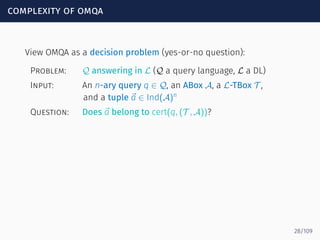


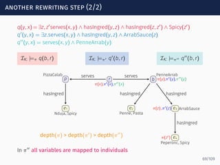
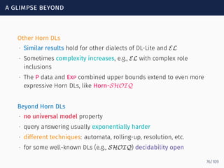


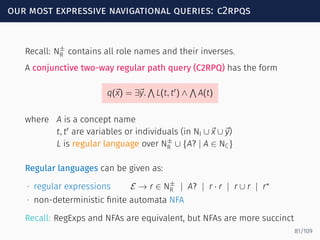
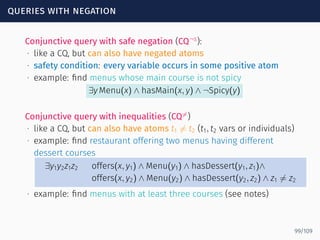
![loops through the anonymous part
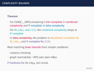
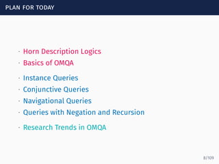
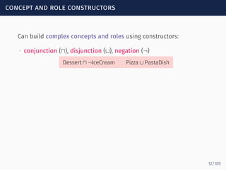
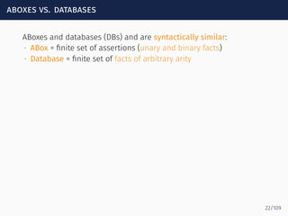
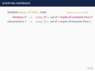
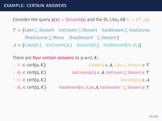
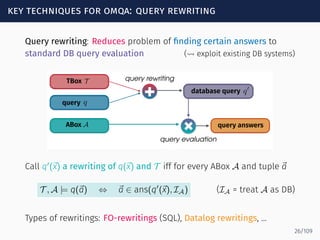
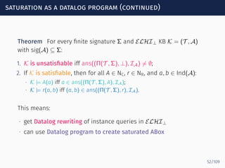
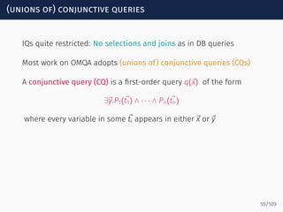
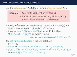
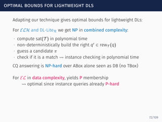
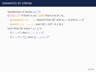
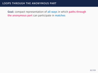
Goal: compact representation of all ways in which paths through
the anonymous part can participate in matches
s0 s1 sf
serves
hasIngred
ingredOf
−
Spicy?
Σ∗
We use NFA representation
We write M ∈ Loopα[s, s′
] iff a ∈ MIK
implies the existence of a path
p below a that takes the NFA α from s to s′
, e.g.,
85/109](https://image.slidesharecdn.com/ontology-mediated-query-answering-with-data-tractable-description-logics-160324104954/85/Ontology-mediated-query-answering-with-data-tractable-description-logics-184-320.jpg)
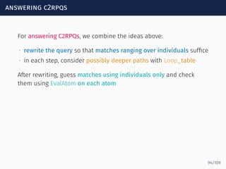
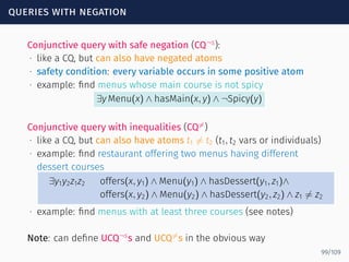
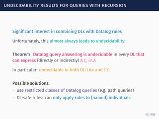
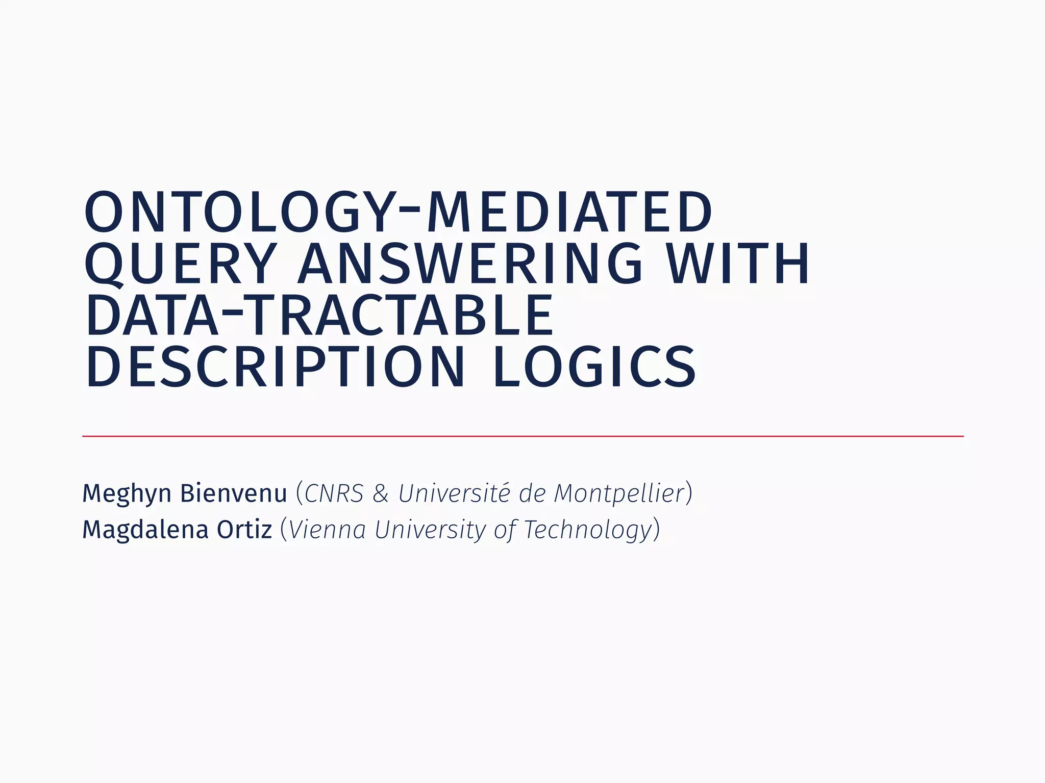
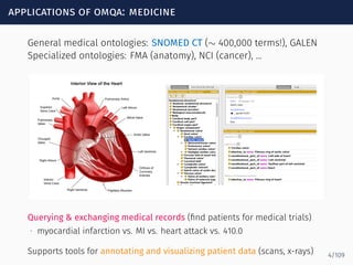
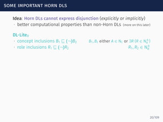
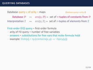
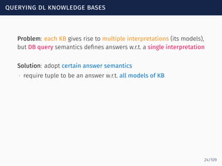
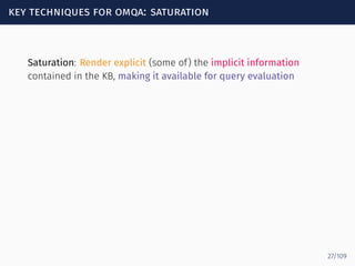
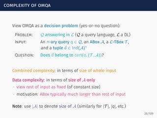
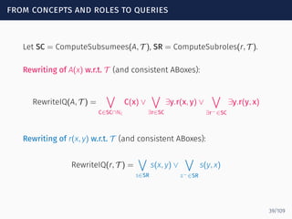
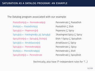
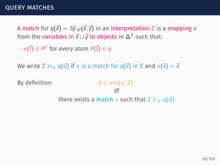
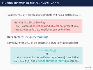
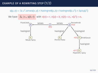
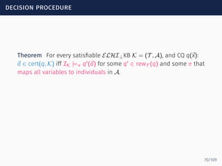
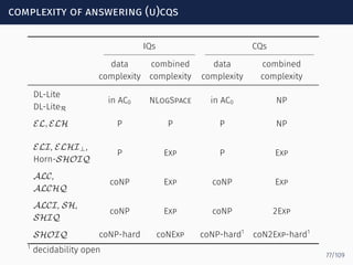
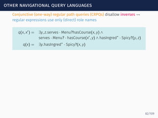
![loops through the anonymous part
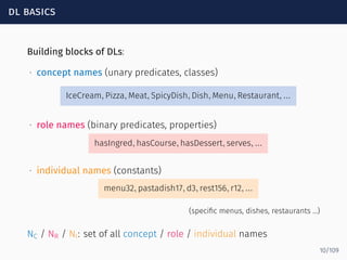
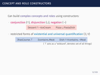
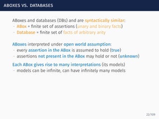
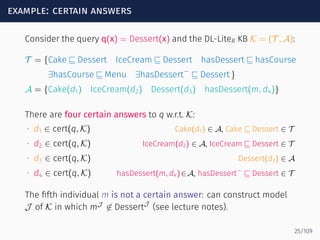
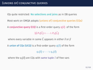
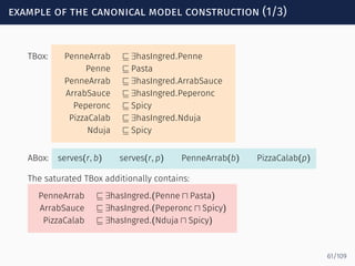
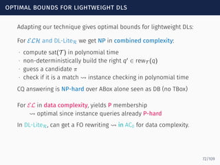
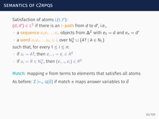
Goal: compact representation of all ways in which paths through
the anonymous part can participate in matches
s0 s1 sf
serves
hasIngred
ingredOf
−
Spicy?
Σ∗
We use NFA representation
We write M ∈ Loopα[s, s′
] iff a ∈ MIK
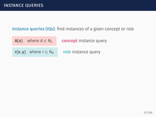
implies the existence of a path
p below a that takes the NFA α from s to s′
, e.g.,
PenneArrab ∈ Loopα[s1, sf]
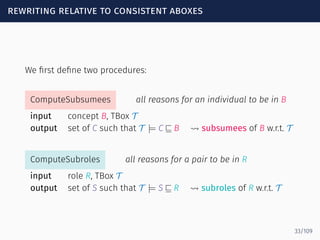
because of
PenneArrab ⊑ ∃hasIngred.ArrabSauce
ArrabSauce ⊑ ∃hasIngred.(Peperonc ⊓ Spicy)
85/109](https://image.slidesharecdn.com/ontology-mediated-query-answering-with-data-tractable-description-logics-160324104954/85/Ontology-mediated-query-answering-with-data-tractable-description-logics-185-320.jpg)
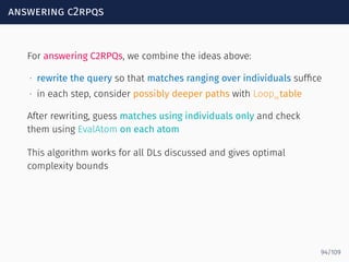
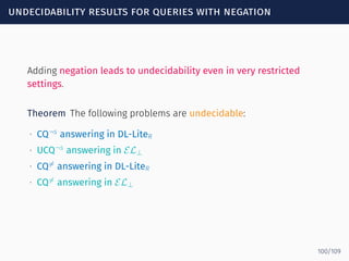
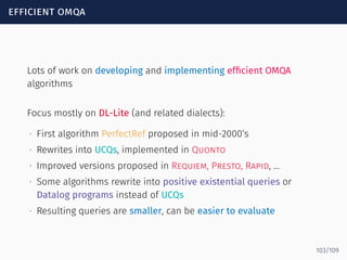
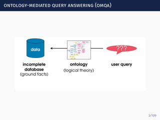
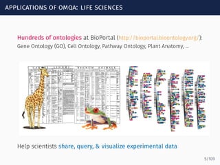
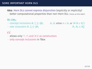
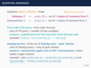
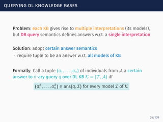
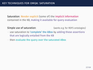
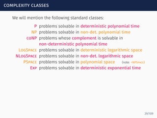
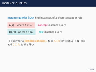
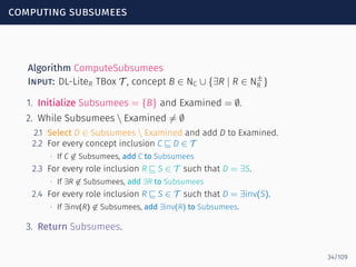
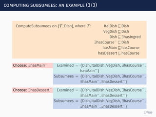
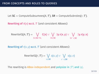
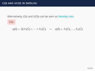
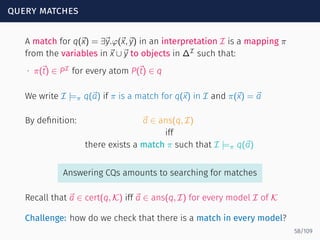
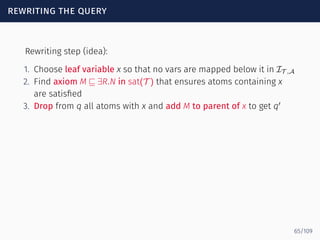
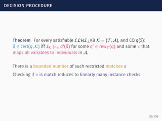
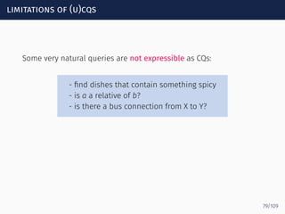
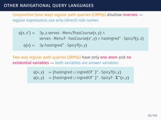
![computing the loop table
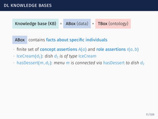
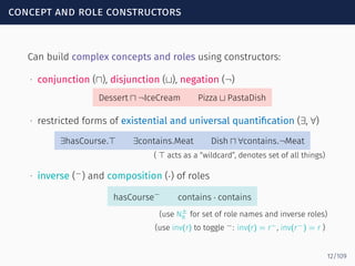
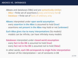
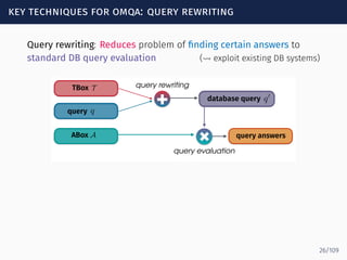
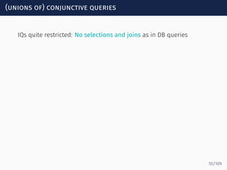
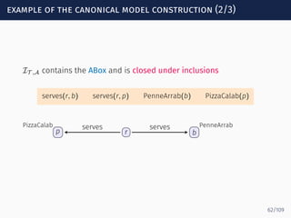
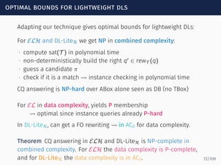
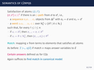
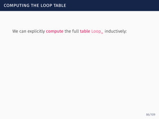
We can explicitly compute the full table Loopα inductively:
if s is a state then Loopα[s, s] = NC
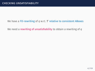
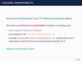
if M1 ∈ Loopα[s1, s2] and
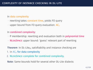
M2 ∈ Loopα[s2, s3]
then M1 ⊓ M2 ∈ Loopα[s1, s3]
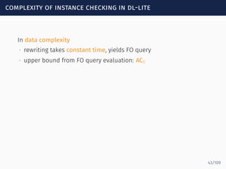
if T |= C1 ⊓ · · · ⊓ Cn ⊑ A and
(s1, A?, s2) ∈ δ
then C1 ⊓ · · · ⊓ Cn ∈ Loopα[s1, s2]
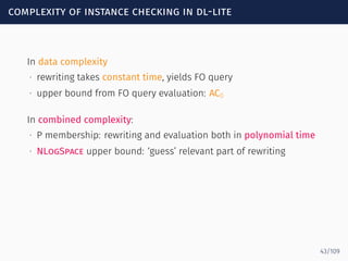
if T |= C1 ⊓ · · · ⊓ Cn ⊑ ∃R.D,
T |= R ⊑ R′
, T |= R ⊑ R′′
,
(s1, R′
, s2) ∈ δ,
D ∈ Loopα[s2, s3], and
(s3, R′′−
, s4) ∈ δ
then C1 ⊓ · · · ⊓ Cn ∈ Loopα[s1, s4]
86/109](https://image.slidesharecdn.com/ontology-mediated-query-answering-with-data-tractable-description-logics-160324104954/85/Ontology-mediated-query-answering-with-data-tractable-description-logics-187-320.jpg)
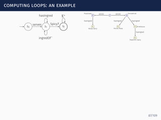
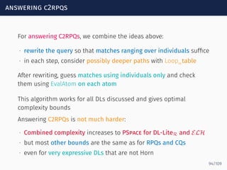
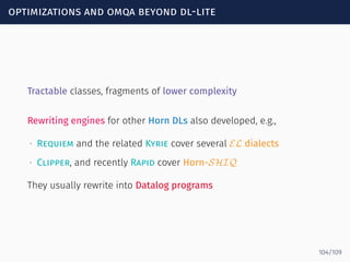
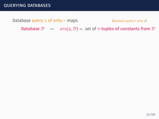
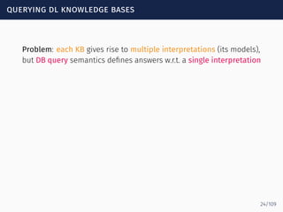
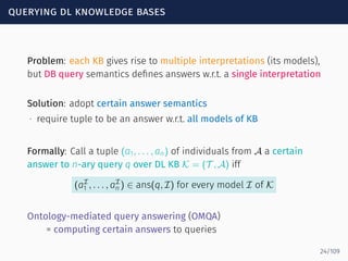
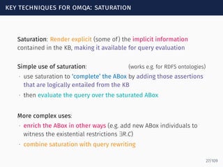
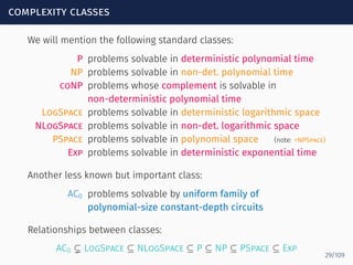
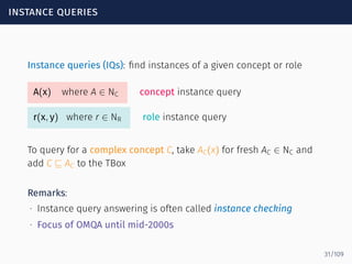
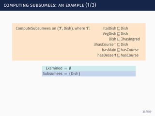
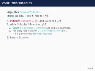
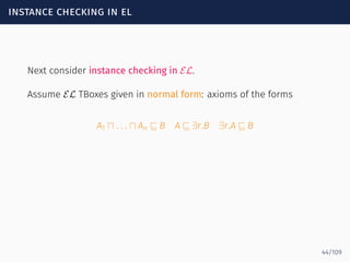
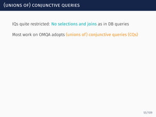
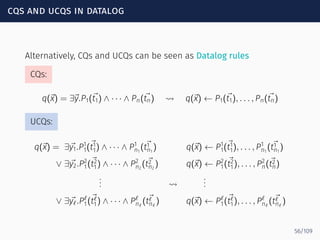
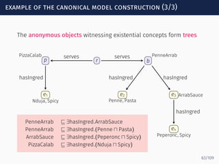
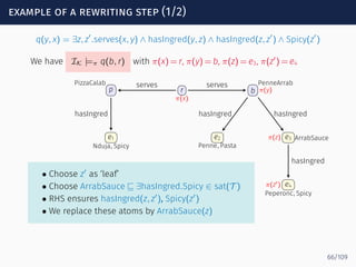
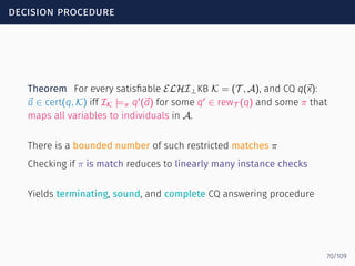
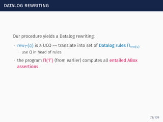
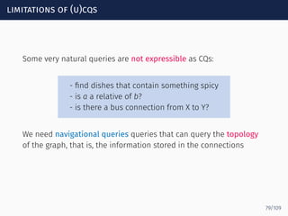
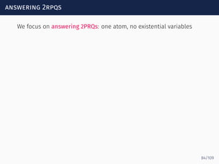
![computing loops: an example
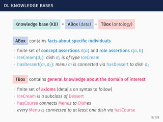
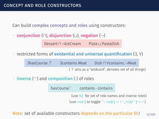
s0 s1 sf
serves
hasIngred
ingredOf
−
Spicy?
Σ∗ rp
PizzaCalab
b
PenneArrab
e1
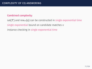
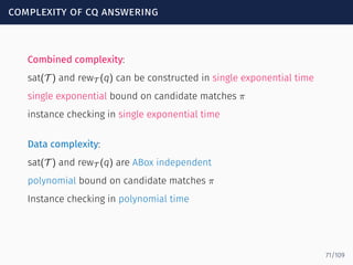
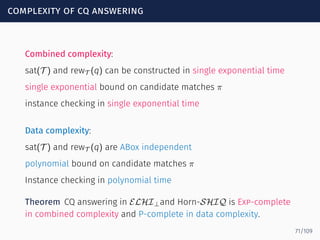
Nduja, Spicy
e2
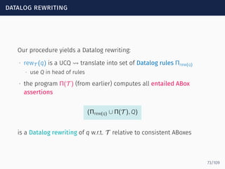
Penne, Pasta
e3 ArrabSauce
e4
Peperonc, Spicy
serves serves
hasIngred hasIngred hasIngred
hasIngred
∙ Peperonc ∈ Loopα[s1, sf] because (s1, Spicy?, sf) ∈ δ and
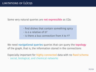
Peperonc ⊑ Spicy
87/109](https://image.slidesharecdn.com/ontology-mediated-query-answering-with-data-tractable-description-logics-160324104954/85/Ontology-mediated-query-answering-with-data-tractable-description-logics-189-320.jpg)
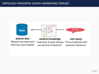
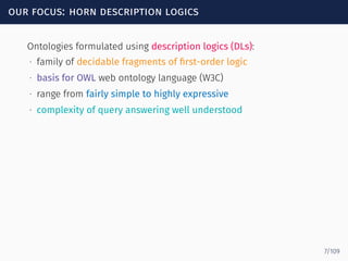
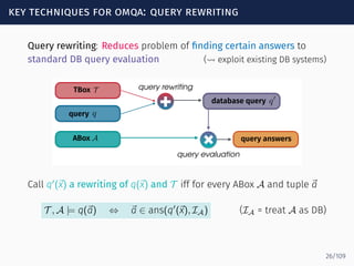
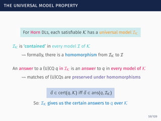
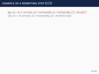
![computing loops: an example
s0 s1 sf
serves
hasIngred
ingredOf
−
Spicy?
Σ∗ rp
PizzaCalab
b
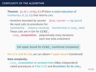
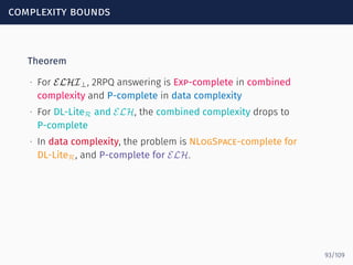
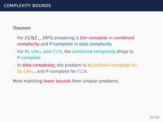
PenneArrab
e1
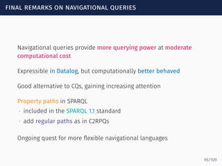
Nduja, Spicy
e2
Penne, Pasta
e3 ArrabSauce
e4
Peperonc, Spicy
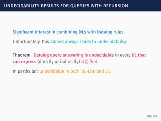
serves serves
hasIngred hasIngred hasIngred
hasIngred
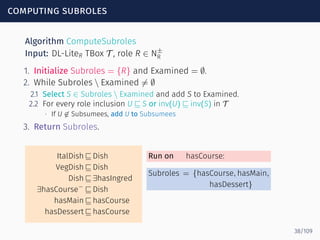
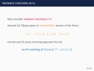
∙ Peperonc ∈ Loopα[s1, sf] because (s1, Spicy?, sf) ∈ δ and
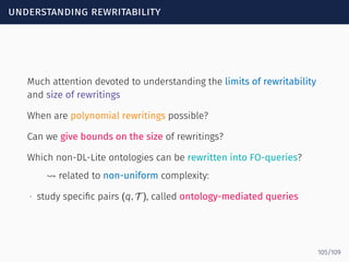
Peperonc ⊑ Spicy
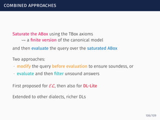
∙ ArrabSauce ∈ Loopα[s1, sf] because
(s1, hasIngred, s1), (sf, hasIngred−
, sf) ∈ δ and
ArrabSauce ⊑ ∃hasIngred.Peperonc
Peperonc ∈ Loopα[s1, sf]
87/109](https://image.slidesharecdn.com/ontology-mediated-query-answering-with-data-tractable-description-logics-160324104954/85/Ontology-mediated-query-answering-with-data-tractable-description-logics-190-320.jpg)
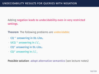
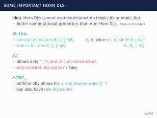
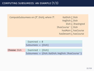
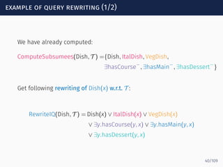
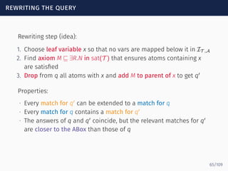
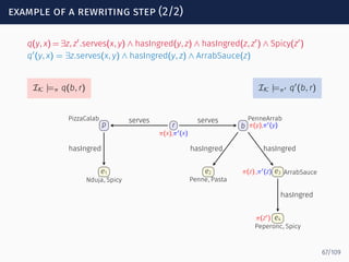
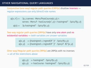
![computing loops: an example
s0 s1 sf
serves
hasIngred
ingredOf
−
Spicy?
Σ∗ rp
PizzaCalab
b
PenneArrab
e1
Nduja, Spicy
e2
Penne, Pasta
e3 ArrabSauce
e4
Peperonc, Spicy
serves serves
hasIngred hasIngred hasIngred
hasIngred
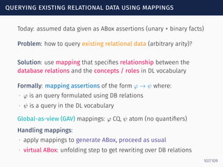
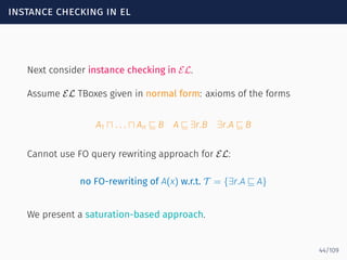
∙ Peperonc ∈ Loopα[s1, sf] because (s1, Spicy?, sf) ∈ δ and
Peperonc ⊑ Spicy
∙ ArrabSauce ∈ Loopα[s1, sf] because
(s1, hasIngred, s1), (sf, hasIngred−
, sf) ∈ δ and
ArrabSauce ⊑ ∃hasIngred.Peperonc
Peperonc ∈ Loopα[s1, sf]
∙ PenneArrab ∈ Loopα[s1, sf] because
(s1, hasIngred, s1), (sf, hasIngred−
, sf) ∈ δ and
PenneArrab ⊑ ∃hasIngred.ArrabSauce
ArrabSauce ∈ Loopα[s1, sf]
87/109](https://image.slidesharecdn.com/ontology-mediated-query-answering-with-data-tractable-description-logics-160324104954/85/Ontology-mediated-query-answering-with-data-tractable-description-logics-191-320.jpg)
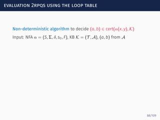
![evaluation 2rpqs using the loop table
Non-deterministic algorithm to decide (a, b) ∈ cert(α(x, y), K)
Input: NFA α = (S, Σ, δ, s0, F), KB K = (T , A), (a, b) from A
∙ After checking consistency, we start from (a, s0)
∙ At pair (c, s), guess new pair (d, s′
) together with one of:
∙ transition (s, σ, s′
) a σ-step from c to d in ABox
⇝ check if (c, d) ∈ σI
∙ concepts M in Loopα[s, s′
] stay at same individual, and jump to s′
⇝ check if c = d ∈ MI
∙ Exit when we get pair (b, sf)
∙ Use counter to ensure termination (only need to consider each
pair once)
88/109](https://image.slidesharecdn.com/ontology-mediated-query-answering-with-data-tractable-description-logics-160324104954/85/Ontology-mediated-query-answering-with-data-tractable-description-logics-193-320.jpg)
![evaluation algorithm
Algorithm EvalAtom
Input: NFA α = (S, Σ, δ, s0, F) with Σ ⊆ N±
R ∪ {A? | A ∈ NC}, ELHI⊥ KB
(T , A), (a, b) ∈ Ind(A) × Ind(A)
1. Test whether (T , A) is satisfiable, output yes if not.
2. Initialize current = (a, s0) and count = 0. Set max = |A| · |S| + 1.
3. While count < max and current ̸∈ {(b, sf) | sf ∈ F}
3.1 Let current = (c, s).
3.2 Guess a pair (d, s′
) ∈ Ind(A) × S and either (s, σ, s′
) ∈ δ or
M ∈ Loopα[s, s′
].
3.3 If (s, σ, s′
) was guessed
∙ If σ ∈ N±
R , then verify that T , A |= σ(c, d), and return no if not.
∙ If σ = A?, then verify that c = d and T , A |= A(c), and return no if not.
3.4 If M was guessed, then verify that c = d and that T , A |= B(c) for every
concept name B ∈ M, and return no if not.
3.5 Set current = (d, s′
) and increment count.
4. If current = (b, sf) for some sf ∈ F, return yes. Else return no.
89/109](https://image.slidesharecdn.com/ontology-mediated-query-answering-with-data-tractable-description-logics-160324104954/85/Ontology-mediated-query-answering-with-data-tractable-description-logics-194-320.jpg)
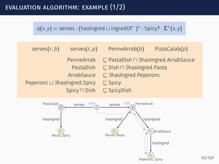
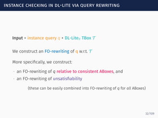
![evaluation algorithm: example (2/2)
serves(r, b) serves(r, p) PenneArrab(b) PizzaCalab(p)
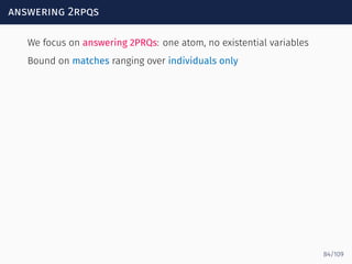
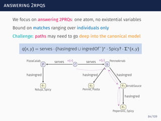
q(x, y) = serves · (hasIngred ∪ ingredOf−
)∗
· Spicy? · Σ∗
(x, y)
s0 s1 sf
serves
hasIngred
ingredOf−
Spicy?
Σ∗Peperonc ∈ Loopα[s1, sf]
ArrabSauce ∈ Loopα[s1, sf]
PenneArrab ∈ Loopα[s1, sf]
91/109](https://image.slidesharecdn.com/ontology-mediated-query-answering-with-data-tractable-description-logics-160324104954/85/Ontology-mediated-query-answering-with-data-tractable-description-logics-196-320.jpg)
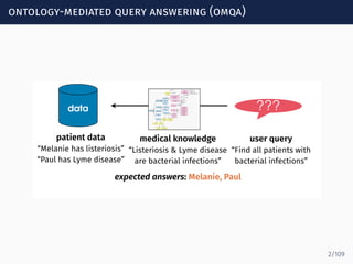
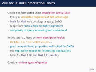
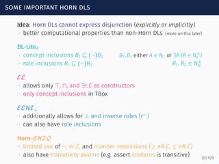
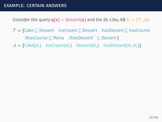
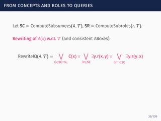
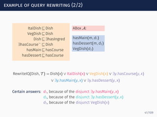
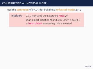
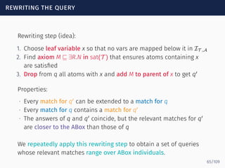
![evaluation algorithm: example (2/2)
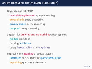
serves(r, b) serves(r, p) PenneArrab(b) PizzaCalab(p)
q(x, y) = serves · (hasIngred ∪ ingredOf−
)∗
· Spicy? · Σ∗
(x, y)
s0 s1 sf
serves
hasIngred
ingredOf−
Spicy?
Σ∗Peperonc ∈ Loopα[s1, sf]
ArrabSauce ∈ Loopα[s1, sf]
PenneArrab ∈ Loopα[s1, sf]
count: 0 1 2
Guess (r, s0) (b, s1) (b, sf)
(s0, serves, s1) ∈ δ PenneArrab ∈ Loopα[s1, sf]
Test (r, b) ∈ servesI
b ∈ PenneArrabI
return yes
91/109](https://image.slidesharecdn.com/ontology-mediated-query-answering-with-data-tractable-description-logics-160324104954/85/Ontology-mediated-query-answering-with-data-tractable-description-logics-197-320.jpg)