Operations Management-II Dr. S.Venkataramanaiah  Assistant Professor OM & QT Area IIM Indore, Pigdamber, Rau Indore- 453 331  Email :  [email_address]
Design of Experiments (DOE) and Taguchi Methods
Objective To understand the relevance of DOE and its applications Implementation of approach
Taguchi’s View of Variation Traditional view is that quality within the LS and US is good and that the cost of quality outside this range is constant, where Taguchi views costs as increasing as variability increases, so seek to achieve zero defects and that will truly minimize quality costs. Tolerances are continuous,  not yes/no Incremental Cost of  Variability High Zero Lower Spec Target Spec Upper Spec Traditional View Incremental Cost of  Variability High Zero Lower Spec Target Spec Upper Spec Taguchi’s View
Taguchi Techniques Experimental design methods to improve product & process design Identify key component & process variables affecting product variation Taguchi  Concepts Quality robustness Quality loss function Target specifications
Quality Robustness Ability to produce products uniformly in adverse manufacturing and environmental conditions Remove the effects of adverse conditions Small variations in materials and process do not destroy product quality
Quality Loss Function Shows that costs increase as the product moves away from what the customer wants Costs include customer dissatisfaction, warranty and service, internal scrap and repair, and costs to society Traditional conformance specifications are too simplistic
Shows social cost ($) of deviation from target value Assumptions Most measurable quality characteristics (e.g., length, weight) have a target value Deviations from target value are undesirable Equation:  L = D 2 C L = Loss ($); D = Deviation; C = Cost Quality Loss Function
Quality Loss Function and its distribution  Low loss High loss Frequency Lower Target Upper Specification Loss (to producing organization, customer, and society) Quality Loss Function (a) Unacceptable Poor Fair Good Best Target-oriented quality yields more product in the “best” category Target-oriented quality brings products toward the target value Conformance-oriented quality keeps product within three standard deviations Distribution of specifications for product produced
The specifications for the diameter of a gear are  25.00 ± 0.25 mm .  If the diameter is out of specification, the gear must be scrapped at a cost of  $4.00.  What is the  loss function ? Quality Loss Function Example © 1984-1994 T/Maker Co.
L = D 2 C = (X - Target) 2 C  L = Loss ($); D = Deviation; C = Cost 4.00 = (25.25 - 25.00) 2 C Item scrapped if greater than 25.25  (USL = 25.00 + 0.25) with a cost of $4.00 C = 4.00 / (25.25 - 25.00) 2  = 64 L = D 2   •  64 = (X - 25.00) 2 64 Enter various X values to obtain L & plot Quality Loss Function Solution
Aspects of processes Aspects in Manufacturing and related Processes Design Issues   Focus on Product Specifications Step Loss Function Control Issues Statistical Process Control Control Charts Keeping Product Performance within Specifications   Inspections Acceptance Sampling Screening: 100% Inspection
Overview of Taguchi Method   Off-Line Quality Control (Taguchi Method) Emphasis on Design Issues for Quality Improvement Process Optimization Optimization Techniques Experimental Design
Overview of Taguchi Method Contributions of Off-Line Quality Control Significance on Process Optimization Focus on Process Variability Quadratic Quality Loss Function Inclusion of Noise Factors Signal-to-Noise (SN) Ratio Process Robust to External Noises Proactive & Cost-Effective Approach Process Optimization from Design Stage Comprehensive Set of Tools for Quality Improvement Wide Applicability
Overview of Taguchi Method Drawbacks of Off-Line Quality Control Inefficient Optimization Metric (SN ratio) Lack of Flexibility in Modeling Design Variables Lack of Economy in Experimental Design Plan Crossed Array Difficulty Associated with Estimating Interactions among Control Factors
Lack of Sequential Search for Optimum Interdependency Among Design Modules Parameter and Tolerance Design Iterative Optimization Procedures Overview of Taguchi Method
Design Modules:  System, Parameter and Tolerance System  Design Parameter Design Tolerance  Design
Integrated Design optimization Need for Integrating Individual Design Modules (System, Parameter, and Tolerance Design)   Integration Scheme Depending on the Type of Design Variables: Dynamic/Static
Procedures and Analysis Tools for Design Optimization with Dynamic Design Variables   Procedures and Analysis Tools for Design Optimization with Static Design Variables
DESIGN OF EXPERIMENTS  (DOE)
DESIGN OF EXPERIMENTS   Definitions and basic aspects Factorial Designs Simple application of DOE
DESIGN OF EXPERIMENTS   EXPERIMENT : Is defined as a study in which certain independent variables are manipulated, their effect on one or more dependent variables is determined and the levels of these independent variables are assigned at random to the experimental units in the study. PURPOSE :   To discover something about a particular process (or) to compare the effect of several factors on some phenomena
OBJECTIVE OF  EXPERIMENT: Objective may be either confirmation (verify knowledge about the system). (or) Exploration (study the effect of new conditions on the system).
TERMINOLOGY DEPENDENT VARIABLE:         It is an outcome or response of an experiment.         It is also called as response variable.         Criterion used is also a dependent variable.   INDEPENDENT VARIABLE (OR) FACTORS:         Variables, which are varied in the experiment.         Can be controlled at fixed levels.         Can be varied or set at levels of our interest.         Randomized.         Can be qualitative (or) quantitative.  
LEVELS OF A FACTOR: The variation of independent variable under each factor (or)number of different possible values of a factor. EFFECT OF A FACTOR: Defined as the change of response produced by a change in the level of that factor.   TREATMENT: It means the factor.
DESIGN OF EXPERIMENTS   Design is defined as the selection of parameters and specification of features that would help the creation of a product or process with a predefined expected performance. Robust design aims at finding parameter settings, which would ensure that performance is on  target , minimizing simultaneously the influence of any adverse factors (the noise) that the user may be unable to control economically or eliminate.
Establishing cause-effect relationships scientifically is pivotal in resolving disputes and questions about unsatisfactory performance of products/processes. In the absence of mathematical cause-effect models, statistically designed experiments are the best for empirically discovering cause-effect relationships.
DOE -PROCEDURE   1. EXPERIMENT Statement of the problem Choice of dependent or response variable Selection of factors to be varied Choice of levels of these factors  
DESIGN No of observations Order of experimentation Method of randomization Mathematical model to describe the experiment Hypothesis to be tested.   ANALYSIS Data collection and processing Computation of test statistics Interpretation of results DOE -PROCEDURE
EXAMPLE OF AN EXPERIMENT Studying the effect of two different hardening processes, oil quenching and salt water quenching on an aluminium alloy.   OBJECTIVE:  To determine the quenching solution that produces the maximum hardness.    PROCEDURE: The experimenter decides to subject a number of alloy specimens to each quenching solution and measure the hardness of the specimens after quenching. The average hardness of the specimens treated in each quenching solution will be used to determine the best solution.
Questions: Do you have only two solutions? Any other factors affect the hardness? How many specimens to be tested? How do you assign the specimens to the two solutions? What is the order of data collection? What method of data analysis to use? What difference in average hardness will be considered important?
STATISTICAL DESIGN OF AN EXPERIMENT   The process of planning the experiment so that appropriate data collected which shall be analyzed by statistical methods resulting in valid and objective conclusions.  Two aspects of experimental problem: The design of the experiment The statistical analysis of the data
Three basic principles of design: Replication:   Repetition of the basic experiment I.e., obtaining the response from the same  experimental set-up once again Used to obtain experimental error Permits the experimenter to obtain a precise estimate of the factor.
Three basic principles of design Randomization: The allocation of the experimental units (material) and the order of experimentation (trails) are randomly determined. Statistical methods require that the observations (or error) are independently distributed random variables. Randomization meets this requirement. It also assists in averaging out the effects of extraneous factors that may be present.
Blocking: Is a technique used to increase the precision of an experiment.  A block is a portion of the experimental material that should be more homogeneous than the entire set of material.  Blocking involves making comparisons among the conditions of interest in the experiment within each block.  It is also a restriction on complete randomization. Three basic principles of design
DESIGN OF EXPERIMENTS CONVENTIONAL TEST STRATERGIES One factor experiments Determining the effect of one factor keeping all other factors constant   Y2 * * A2 2 Y1 * * A1 1 Average  Test Result Factor Level Trial
Several Factors one at a time Y4 * * * 2 1 1 4 Y3 * * * 1 2 1 3 Y2 * * * 1 1 2 2 Y1 * * * 1 1 1 1 C B A Average Result Factors Trial
Several factors all at the same time Factorial Experiments Fractional Factorial Experiments Y2 * * * 2 2 2 2 2 Y1 * * * 1 1 1 1 1 D C B A Average Result Factor and Level Trial
FACTORIAL EXPERIMENTATTIONS A factorial design is one in which all possible combinations of the levels of factors are investigated E.g. Factor A at 2 levels and Factor B at 3 levels  Total possible combinations are six (2x3) B1 B1 A1 B2 A2 B2 B3 B3 Factor A at a levels and Factor B at b levels
FACTORIAL EXPERIMENTATTIONS Total possible combinations ab Factorial designs are more efficient designs Factorial designs are necessary when interactions are present Factorial designs allow effects of a factor to be estimated at several levels of the other factors TYPES OF FACTORIAL DESIGNS Full Factorial Designs Fractional Factorial Designs
FULL FACTORIAL EXPERIMENTATION An experimental design in which all the possible combinations are tested Eg. To study the effect of two factors, feed rate (A) and cutting speed (B) on the finish of a machined shaft. Assume each to be at 2 levels.  All possible combinations A1 B1, A1B2, A2B1, A2B2 Effect of Factor A = ( Y4+Y3)/2-(Y2+Y1)/2 Effect of Factor B = ( Y4+Y2)/2-(Y3+Y1)/2 FULL FACTORIAL EXPERIMENTS Both factors and interaction effects can be studied Have high confidence Y4 2 2 4 Y3 1 2 3 Y2 2 1 2 Y1 1 1 1 B A AVERAGE RESULTS FACTORS AND FACTOR LEVELS TRIAL NUMBER
FULL FACTORIAL EXPERIMENTATION To conduct a full factorial experiment with two factors each at 2 levels, it is required to do 4 trials (2 2 ) In general, Total number of trials to be conducted for full factorial experiments with ‘a’ factors at ‘b’ levels each is b a
Consider a case with 7 factors at 2 levels each. It would require 2 7  trials = 128 trails Usual time and financial limitations preclude the use of Full Factorial experimentation most of the time  How one can efficiently and economically investigate these factors ? FULL FACTORIAL EXPERIMENTATION
FRACTIONAL FACTORIAL EXPERIMENTS Fractional Factorial Experiments (FFE) are more efficient test plans FFE’s use only a portion of the total possible combinations to estimate the Main factor effects and some, not all of the interactions Simplest FFE designs are those with factors are at 2 levels example  One-half FFE One-quarter FFE One-eighth FFE One-sixteenth FFE  etc.
FACTORIAL  DESIGNS MAIN EFFECT : Change in  response  produced by a change in the level of the factor B A FIG. 1 FIG. 2 FIG 1 Avg. effect of A = [(40-20)+(52 –30)]/2 = 21 Avg. effect of B = [(52-40)+(30-20)]/2 = 11 B A L L H H . . . . 20 40 50 12 L L H H . . . . 20 40 30 52
INTERACTION  EFFECT The difference in response between the levels of one factor is not the same at all levels of the other factors. At low level of ‘B’, the ‘A’ effect is : 50-20=30 At high level of ‘B’, the ‘A’ effect is : 12-40=-28 The avg. interaction effect ‘AB’ = (-28-30)/2 = -29  RESPONSE RESPONSE FACTOR  A FACTOR  A A1B1 A1B1 A1B2 A1B2 A2B2 A2B2 A2B1 A2B1 NO SIGNIFIANT INTERACTION SIGNIFIANT INTERACTION
INTERACTION  EFFECT When interaction is maximum, then corresponding main effects have little  practical meaning. However, the effect of A at different levels of factor B is significant  Ex. Effect of A is : (50+12)/2-(20+40)/2= 1 may lead to a conclusion that A has no effect ( Is it correct?) Factor A has an effect and it depends on the level of factor B. Hence the knowledge about interaction between AB is more useful than main effects. The interaction effect of one factor (let A) with levels of other factors fixed to draw conclusions. Information on both can be studied by varying one at a time. The effect of changing factor A (B is fixed) is given by A + B -  – A - B - B A L L H H . . . A - B - A + B - A + B + B A L L H H . . . . 20 40 50 12
THE TWO FACTOR FACTORIAL DESIGN Y ijk  =  µ  + A i  + B j  + Ab ij  + C (ij)k where  A and B are the two Factors i = 1,2………a levels of A j = 1,2………b levels of B k = 1,2…….. n observations per cell SSTotal = SSA+ SSB+ SSAB+ SSE df: (abn-1) = (a-1) + (b-1) + (a-1)(b-1) + ab(n-1)
THE TWO FACTOR FACTORIAL DESIGN FORMULA FOR SS: CF = T 2 /N  ; (N=abn) and T= Grand total SS Total  =  Σ Σ Σ (Y ijk ) 2  - CF  ;  i,j,k ranges from 1 to a,b,n respectively SS A =  Σ  (Ti ) 2 /bn – CF  ; i ranges from 1 to a SS B =  Σ  (Tj ) 2 /an – CF  ; j ranges from 1 to b SS AB =  Σ  (Tij ) 2 /n – CF – SSA - SSB  SS E = SS Total  – (SS A + SS B + SS AB )
H 0  : No significant difference If F 0 >  F x,v1,v2 ,  reject H 0  abn-1 TOTAL MS E =SS E / ab(n-1) ab(n-1) SS E Error MS AB /MS E MS Ab =SS AB / (a-1)(b-1) (a-1)(b-1) SS AB AB MS B /MS E MS B =SS B /b-1 b-1 SS B B MS A /MS E MS A =SS A /a-1 a-1 SS A A F 0 Mean  square Degrees of freedom Sum of squares Source of variation
TWO FACTOR EXPERIMENT : AN ILLUSTRATION Life Data (Hrs) for a battery Design   T=3799 770 1291 1738 Ti 60 82 139 150 160 168 1501 342 104 96 583 120 174 576 110 138 3 45 58 115 106 126 159 1300 198 70 25 79 122 136 623 188 150 2 58 82 75 80 180 74 998 230 70 20 229 40 34 539 155 130 1 125 70 15 T j Temperature (A) Material Type (B)
SS Total   = sum of Y 2 ijk  – CF  i,j,k = 1…………a,b,x respectively = 130 2 +155 2 + 74 2 +………+60 2 - 3799 2 /36 = 77646.97 SS A  = ((1738) 2 +(1291) 2 +(770) 2 )/12) – ((3799) 2 /36) = 39118.72  SS B  = ((998) 2 +(1300) 2 +(1501) 2 )/12) – ((3799) 2 /36) = 10683.72 SS AB  =¼*(539 2 +229 2 +………342 2 )–((3799) 2 /36)-SSA -SSB = 9613.78 SS E  = SS Total  - SS A  - SS B  - SS AB  = 18230.75
ANOVA : Battery Life F 0.05, 4,27  = 2.73 F 0.05, 2,27 = 3.35 35 77646.97 Total  675.21 27 18230.75 Error  3.56  S 2403.44 4 9613.78 Interaction (AB)  7.91  S 5341.86 2 10683.72 Material Type (B) 28.97  S 19559.36 2 39118.72 Temperature (A) F O Mean Square Degrees of freedom Sum of Squares Source of variation
Material type 3 gives best results if we want less loss of life as temperature changes Avg Response of Treatments There exists significant interaction Longer life is attainable at low temperature regardless of type of material and M2 shows better life than other two When temperature change from low to medium the life increases with material 3 At higher temperature, life is shorter and M3 better at higher temperature. M1 shows same life at both medium and higher temperature 25 125 70 15 175 150 125 100 75 50 0 M1 M2 M3 Temperature Avg Life
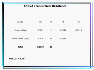
A SINGLE FACTORS EXPERIMENT (one-way ANOVA) FABRIC WEAR RESISTANCE DATA T… = 38.41 CF = T 2 /N SS TOTAL  = SS FACTOR  + SS E SS TOTAL  = 1.93 2 + 2.38 2 +……+ 2.25 2  –(38.41) 2 /16 = 0.7639 SS FACTOR  = (8.76 2 + 10.72 2 + 9.67 2 + 9.26 2 )/4 – CF = 0.5201 Col. Total 9.26 9.67 10.72 8.76 2.25 2.28 2.70 2.25 2.28 2.31 2.75 2.20 2.40 2.68 2.72 2.38 2.33 2.40 2.55 1.93 D C B A TYPE OF FABRIC
ANOVA : Fabric Wear Resistance F 0.05, 3,12  = 3.49 15 0.7639 Total  0.0203 12 0.2438 Within Fabrics (Error) 8.54  S  0.1734 3 0.5201 Between Fabrics F O MS df SS Source
NEWMAN-KEUAL’S TEST Fabric Wear Resistance Problem  Arrange the means in ascending order 2.19 2.32 2.42 2.68 A D C B Compute standard error of mean S yj  =  MSE / x j  =  0.0203/4  = 0.0712 From studentized range Table, at alpha = 5%, for x 2  = 12 df, the ranges are  P :  2 3 4 Ranges:  3.08 3.77 4.20
Obtain Least significant ranges by multiplying the ranges by the standard error P: 2 3 4 LSR: 0.22 0.27 0.30 Compare the observed difference in all possible pairs of means with the LSRs to determine the significance
Conclusions  Taguchi methods are very useful in addressing the design quality issues It helps in determining the levels that results in overall best combination

om

  • 1.
    Operations Management-II Dr.S.Venkataramanaiah Assistant Professor OM & QT Area IIM Indore, Pigdamber, Rau Indore- 453 331 Email : [email_address]
  • 2.
    Design of Experiments(DOE) and Taguchi Methods
  • 3.
    Objective To understandthe relevance of DOE and its applications Implementation of approach
  • 4.
    Taguchi’s View ofVariation Traditional view is that quality within the LS and US is good and that the cost of quality outside this range is constant, where Taguchi views costs as increasing as variability increases, so seek to achieve zero defects and that will truly minimize quality costs. Tolerances are continuous, not yes/no Incremental Cost of Variability High Zero Lower Spec Target Spec Upper Spec Traditional View Incremental Cost of Variability High Zero Lower Spec Target Spec Upper Spec Taguchi’s View
  • 5.
    Taguchi Techniques Experimentaldesign methods to improve product & process design Identify key component & process variables affecting product variation Taguchi Concepts Quality robustness Quality loss function Target specifications
  • 6.
    Quality Robustness Abilityto produce products uniformly in adverse manufacturing and environmental conditions Remove the effects of adverse conditions Small variations in materials and process do not destroy product quality
  • 7.
    Quality Loss FunctionShows that costs increase as the product moves away from what the customer wants Costs include customer dissatisfaction, warranty and service, internal scrap and repair, and costs to society Traditional conformance specifications are too simplistic
  • 8.
    Shows social cost($) of deviation from target value Assumptions Most measurable quality characteristics (e.g., length, weight) have a target value Deviations from target value are undesirable Equation: L = D 2 C L = Loss ($); D = Deviation; C = Cost Quality Loss Function
  • 9.
    Quality Loss Functionand its distribution Low loss High loss Frequency Lower Target Upper Specification Loss (to producing organization, customer, and society) Quality Loss Function (a) Unacceptable Poor Fair Good Best Target-oriented quality yields more product in the “best” category Target-oriented quality brings products toward the target value Conformance-oriented quality keeps product within three standard deviations Distribution of specifications for product produced
  • 10.
    The specifications forthe diameter of a gear are 25.00 ± 0.25 mm . If the diameter is out of specification, the gear must be scrapped at a cost of $4.00. What is the loss function ? Quality Loss Function Example © 1984-1994 T/Maker Co.
  • 11.
    L = D2 C = (X - Target) 2 C L = Loss ($); D = Deviation; C = Cost 4.00 = (25.25 - 25.00) 2 C Item scrapped if greater than 25.25 (USL = 25.00 + 0.25) with a cost of $4.00 C = 4.00 / (25.25 - 25.00) 2 = 64 L = D 2 • 64 = (X - 25.00) 2 64 Enter various X values to obtain L & plot Quality Loss Function Solution
  • 12.
    Aspects of processesAspects in Manufacturing and related Processes Design Issues Focus on Product Specifications Step Loss Function Control Issues Statistical Process Control Control Charts Keeping Product Performance within Specifications Inspections Acceptance Sampling Screening: 100% Inspection
  • 13.
    Overview of TaguchiMethod Off-Line Quality Control (Taguchi Method) Emphasis on Design Issues for Quality Improvement Process Optimization Optimization Techniques Experimental Design
  • 14.
    Overview of TaguchiMethod Contributions of Off-Line Quality Control Significance on Process Optimization Focus on Process Variability Quadratic Quality Loss Function Inclusion of Noise Factors Signal-to-Noise (SN) Ratio Process Robust to External Noises Proactive & Cost-Effective Approach Process Optimization from Design Stage Comprehensive Set of Tools for Quality Improvement Wide Applicability
  • 15.
    Overview of TaguchiMethod Drawbacks of Off-Line Quality Control Inefficient Optimization Metric (SN ratio) Lack of Flexibility in Modeling Design Variables Lack of Economy in Experimental Design Plan Crossed Array Difficulty Associated with Estimating Interactions among Control Factors
  • 16.
    Lack of SequentialSearch for Optimum Interdependency Among Design Modules Parameter and Tolerance Design Iterative Optimization Procedures Overview of Taguchi Method
  • 17.
    Design Modules: System, Parameter and Tolerance System Design Parameter Design Tolerance Design
  • 18.
    Integrated Design optimizationNeed for Integrating Individual Design Modules (System, Parameter, and Tolerance Design) Integration Scheme Depending on the Type of Design Variables: Dynamic/Static
  • 19.
    Procedures and AnalysisTools for Design Optimization with Dynamic Design Variables Procedures and Analysis Tools for Design Optimization with Static Design Variables
  • 20.
  • 21.
    DESIGN OF EXPERIMENTS Definitions and basic aspects Factorial Designs Simple application of DOE
  • 22.
    DESIGN OF EXPERIMENTS EXPERIMENT : Is defined as a study in which certain independent variables are manipulated, their effect on one or more dependent variables is determined and the levels of these independent variables are assigned at random to the experimental units in the study. PURPOSE : To discover something about a particular process (or) to compare the effect of several factors on some phenomena
  • 23.
    OBJECTIVE OF EXPERIMENT: Objective may be either confirmation (verify knowledge about the system). (or) Exploration (study the effect of new conditions on the system).
  • 24.
    TERMINOLOGY DEPENDENT VARIABLE:       It is an outcome or response of an experiment.        It is also called as response variable.        Criterion used is also a dependent variable.   INDEPENDENT VARIABLE (OR) FACTORS:        Variables, which are varied in the experiment.        Can be controlled at fixed levels.        Can be varied or set at levels of our interest.        Randomized.        Can be qualitative (or) quantitative.  
  • 25.
    LEVELS OF AFACTOR: The variation of independent variable under each factor (or)number of different possible values of a factor. EFFECT OF A FACTOR: Defined as the change of response produced by a change in the level of that factor.   TREATMENT: It means the factor.
  • 26.
    DESIGN OF EXPERIMENTS Design is defined as the selection of parameters and specification of features that would help the creation of a product or process with a predefined expected performance. Robust design aims at finding parameter settings, which would ensure that performance is on target , minimizing simultaneously the influence of any adverse factors (the noise) that the user may be unable to control economically or eliminate.
  • 27.
    Establishing cause-effect relationshipsscientifically is pivotal in resolving disputes and questions about unsatisfactory performance of products/processes. In the absence of mathematical cause-effect models, statistically designed experiments are the best for empirically discovering cause-effect relationships.
  • 28.
    DOE -PROCEDURE 1. EXPERIMENT Statement of the problem Choice of dependent or response variable Selection of factors to be varied Choice of levels of these factors  
  • 29.
    DESIGN No ofobservations Order of experimentation Method of randomization Mathematical model to describe the experiment Hypothesis to be tested.   ANALYSIS Data collection and processing Computation of test statistics Interpretation of results DOE -PROCEDURE
  • 30.
    EXAMPLE OF ANEXPERIMENT Studying the effect of two different hardening processes, oil quenching and salt water quenching on an aluminium alloy.   OBJECTIVE: To determine the quenching solution that produces the maximum hardness.   PROCEDURE: The experimenter decides to subject a number of alloy specimens to each quenching solution and measure the hardness of the specimens after quenching. The average hardness of the specimens treated in each quenching solution will be used to determine the best solution.
  • 31.
    Questions: Do youhave only two solutions? Any other factors affect the hardness? How many specimens to be tested? How do you assign the specimens to the two solutions? What is the order of data collection? What method of data analysis to use? What difference in average hardness will be considered important?
  • 32.
    STATISTICAL DESIGN OFAN EXPERIMENT The process of planning the experiment so that appropriate data collected which shall be analyzed by statistical methods resulting in valid and objective conclusions. Two aspects of experimental problem: The design of the experiment The statistical analysis of the data
  • 33.
    Three basic principlesof design: Replication: Repetition of the basic experiment I.e., obtaining the response from the same experimental set-up once again Used to obtain experimental error Permits the experimenter to obtain a precise estimate of the factor.
  • 34.
    Three basic principlesof design Randomization: The allocation of the experimental units (material) and the order of experimentation (trails) are randomly determined. Statistical methods require that the observations (or error) are independently distributed random variables. Randomization meets this requirement. It also assists in averaging out the effects of extraneous factors that may be present.
  • 35.
    Blocking: Is atechnique used to increase the precision of an experiment. A block is a portion of the experimental material that should be more homogeneous than the entire set of material. Blocking involves making comparisons among the conditions of interest in the experiment within each block. It is also a restriction on complete randomization. Three basic principles of design
  • 36.
    DESIGN OF EXPERIMENTSCONVENTIONAL TEST STRATERGIES One factor experiments Determining the effect of one factor keeping all other factors constant Y2 * * A2 2 Y1 * * A1 1 Average Test Result Factor Level Trial
  • 37.
    Several Factors oneat a time Y4 * * * 2 1 1 4 Y3 * * * 1 2 1 3 Y2 * * * 1 1 2 2 Y1 * * * 1 1 1 1 C B A Average Result Factors Trial
  • 38.
    Several factors allat the same time Factorial Experiments Fractional Factorial Experiments Y2 * * * 2 2 2 2 2 Y1 * * * 1 1 1 1 1 D C B A Average Result Factor and Level Trial
  • 39.
    FACTORIAL EXPERIMENTATTIONS Afactorial design is one in which all possible combinations of the levels of factors are investigated E.g. Factor A at 2 levels and Factor B at 3 levels Total possible combinations are six (2x3) B1 B1 A1 B2 A2 B2 B3 B3 Factor A at a levels and Factor B at b levels
  • 40.
    FACTORIAL EXPERIMENTATTIONS Totalpossible combinations ab Factorial designs are more efficient designs Factorial designs are necessary when interactions are present Factorial designs allow effects of a factor to be estimated at several levels of the other factors TYPES OF FACTORIAL DESIGNS Full Factorial Designs Fractional Factorial Designs
  • 41.
    FULL FACTORIAL EXPERIMENTATIONAn experimental design in which all the possible combinations are tested Eg. To study the effect of two factors, feed rate (A) and cutting speed (B) on the finish of a machined shaft. Assume each to be at 2 levels. All possible combinations A1 B1, A1B2, A2B1, A2B2 Effect of Factor A = ( Y4+Y3)/2-(Y2+Y1)/2 Effect of Factor B = ( Y4+Y2)/2-(Y3+Y1)/2 FULL FACTORIAL EXPERIMENTS Both factors and interaction effects can be studied Have high confidence Y4 2 2 4 Y3 1 2 3 Y2 2 1 2 Y1 1 1 1 B A AVERAGE RESULTS FACTORS AND FACTOR LEVELS TRIAL NUMBER
  • 42.
    FULL FACTORIAL EXPERIMENTATIONTo conduct a full factorial experiment with two factors each at 2 levels, it is required to do 4 trials (2 2 ) In general, Total number of trials to be conducted for full factorial experiments with ‘a’ factors at ‘b’ levels each is b a
  • 43.
    Consider a casewith 7 factors at 2 levels each. It would require 2 7 trials = 128 trails Usual time and financial limitations preclude the use of Full Factorial experimentation most of the time How one can efficiently and economically investigate these factors ? FULL FACTORIAL EXPERIMENTATION
  • 44.
    FRACTIONAL FACTORIAL EXPERIMENTSFractional Factorial Experiments (FFE) are more efficient test plans FFE’s use only a portion of the total possible combinations to estimate the Main factor effects and some, not all of the interactions Simplest FFE designs are those with factors are at 2 levels example One-half FFE One-quarter FFE One-eighth FFE One-sixteenth FFE etc.
  • 45.
    FACTORIAL DESIGNSMAIN EFFECT : Change in response produced by a change in the level of the factor B A FIG. 1 FIG. 2 FIG 1 Avg. effect of A = [(40-20)+(52 –30)]/2 = 21 Avg. effect of B = [(52-40)+(30-20)]/2 = 11 B A L L H H . . . . 20 40 50 12 L L H H . . . . 20 40 30 52
  • 46.
    INTERACTION EFFECTThe difference in response between the levels of one factor is not the same at all levels of the other factors. At low level of ‘B’, the ‘A’ effect is : 50-20=30 At high level of ‘B’, the ‘A’ effect is : 12-40=-28 The avg. interaction effect ‘AB’ = (-28-30)/2 = -29 RESPONSE RESPONSE FACTOR A FACTOR A A1B1 A1B1 A1B2 A1B2 A2B2 A2B2 A2B1 A2B1 NO SIGNIFIANT INTERACTION SIGNIFIANT INTERACTION
  • 47.
    INTERACTION EFFECTWhen interaction is maximum, then corresponding main effects have little practical meaning. However, the effect of A at different levels of factor B is significant Ex. Effect of A is : (50+12)/2-(20+40)/2= 1 may lead to a conclusion that A has no effect ( Is it correct?) Factor A has an effect and it depends on the level of factor B. Hence the knowledge about interaction between AB is more useful than main effects. The interaction effect of one factor (let A) with levels of other factors fixed to draw conclusions. Information on both can be studied by varying one at a time. The effect of changing factor A (B is fixed) is given by A + B - – A - B - B A L L H H . . . A - B - A + B - A + B + B A L L H H . . . . 20 40 50 12
  • 48.
    THE TWO FACTORFACTORIAL DESIGN Y ijk = µ + A i + B j + Ab ij + C (ij)k where A and B are the two Factors i = 1,2………a levels of A j = 1,2………b levels of B k = 1,2…….. n observations per cell SSTotal = SSA+ SSB+ SSAB+ SSE df: (abn-1) = (a-1) + (b-1) + (a-1)(b-1) + ab(n-1)
  • 49.
    THE TWO FACTORFACTORIAL DESIGN FORMULA FOR SS: CF = T 2 /N ; (N=abn) and T= Grand total SS Total = Σ Σ Σ (Y ijk ) 2 - CF ; i,j,k ranges from 1 to a,b,n respectively SS A = Σ (Ti ) 2 /bn – CF ; i ranges from 1 to a SS B = Σ (Tj ) 2 /an – CF ; j ranges from 1 to b SS AB = Σ (Tij ) 2 /n – CF – SSA - SSB SS E = SS Total – (SS A + SS B + SS AB )
  • 50.
    H 0 : No significant difference If F 0 > F x,v1,v2 , reject H 0 abn-1 TOTAL MS E =SS E / ab(n-1) ab(n-1) SS E Error MS AB /MS E MS Ab =SS AB / (a-1)(b-1) (a-1)(b-1) SS AB AB MS B /MS E MS B =SS B /b-1 b-1 SS B B MS A /MS E MS A =SS A /a-1 a-1 SS A A F 0 Mean square Degrees of freedom Sum of squares Source of variation
  • 51.
    TWO FACTOR EXPERIMENT: AN ILLUSTRATION Life Data (Hrs) for a battery Design T=3799 770 1291 1738 Ti 60 82 139 150 160 168 1501 342 104 96 583 120 174 576 110 138 3 45 58 115 106 126 159 1300 198 70 25 79 122 136 623 188 150 2 58 82 75 80 180 74 998 230 70 20 229 40 34 539 155 130 1 125 70 15 T j Temperature (A) Material Type (B)
  • 52.
    SS Total = sum of Y 2 ijk – CF i,j,k = 1…………a,b,x respectively = 130 2 +155 2 + 74 2 +………+60 2 - 3799 2 /36 = 77646.97 SS A = ((1738) 2 +(1291) 2 +(770) 2 )/12) – ((3799) 2 /36) = 39118.72 SS B = ((998) 2 +(1300) 2 +(1501) 2 )/12) – ((3799) 2 /36) = 10683.72 SS AB =¼*(539 2 +229 2 +………342 2 )–((3799) 2 /36)-SSA -SSB = 9613.78 SS E = SS Total - SS A - SS B - SS AB = 18230.75
  • 53.
    ANOVA : BatteryLife F 0.05, 4,27 = 2.73 F 0.05, 2,27 = 3.35 35 77646.97 Total 675.21 27 18230.75 Error 3.56 S 2403.44 4 9613.78 Interaction (AB) 7.91 S 5341.86 2 10683.72 Material Type (B) 28.97 S 19559.36 2 39118.72 Temperature (A) F O Mean Square Degrees of freedom Sum of Squares Source of variation
  • 54.
    Material type 3gives best results if we want less loss of life as temperature changes Avg Response of Treatments There exists significant interaction Longer life is attainable at low temperature regardless of type of material and M2 shows better life than other two When temperature change from low to medium the life increases with material 3 At higher temperature, life is shorter and M3 better at higher temperature. M1 shows same life at both medium and higher temperature 25 125 70 15 175 150 125 100 75 50 0 M1 M2 M3 Temperature Avg Life
  • 55.
    A SINGLE FACTORSEXPERIMENT (one-way ANOVA) FABRIC WEAR RESISTANCE DATA T… = 38.41 CF = T 2 /N SS TOTAL = SS FACTOR + SS E SS TOTAL = 1.93 2 + 2.38 2 +……+ 2.25 2 –(38.41) 2 /16 = 0.7639 SS FACTOR = (8.76 2 + 10.72 2 + 9.67 2 + 9.26 2 )/4 – CF = 0.5201 Col. Total 9.26 9.67 10.72 8.76 2.25 2.28 2.70 2.25 2.28 2.31 2.75 2.20 2.40 2.68 2.72 2.38 2.33 2.40 2.55 1.93 D C B A TYPE OF FABRIC
  • 56.
    ANOVA : FabricWear Resistance F 0.05, 3,12 = 3.49 15 0.7639 Total 0.0203 12 0.2438 Within Fabrics (Error) 8.54 S 0.1734 3 0.5201 Between Fabrics F O MS df SS Source
  • 57.
    NEWMAN-KEUAL’S TEST FabricWear Resistance Problem Arrange the means in ascending order 2.19 2.32 2.42 2.68 A D C B Compute standard error of mean S yj = MSE / x j = 0.0203/4 = 0.0712 From studentized range Table, at alpha = 5%, for x 2 = 12 df, the ranges are P : 2 3 4 Ranges: 3.08 3.77 4.20
  • 58.
    Obtain Least significantranges by multiplying the ranges by the standard error P: 2 3 4 LSR: 0.22 0.27 0.30 Compare the observed difference in all possible pairs of means with the LSRs to determine the significance
  • 59.
    Conclusions Taguchimethods are very useful in addressing the design quality issues It helps in determining the levels that results in overall best combination