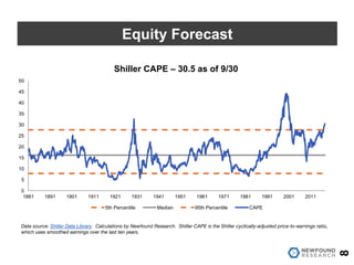
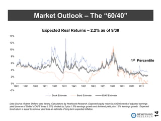
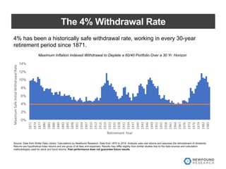
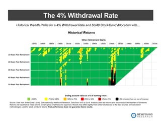
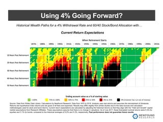
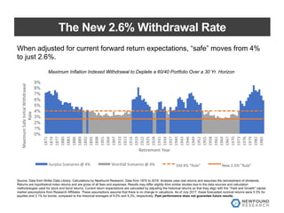
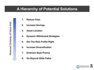
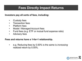
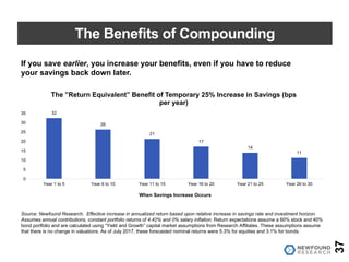
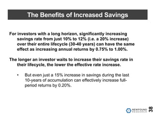
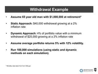
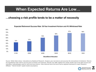
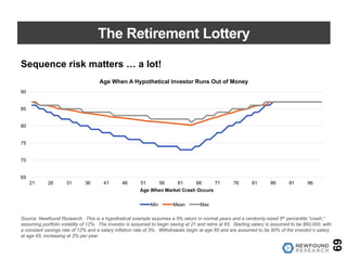
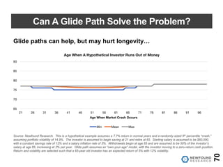
The document discusses strategies for financial planning in a low-return environment, highlighting the challenges of achieving traditional withdrawal rates given current market conditions. It emphasizes the importance of reducing fees, increasing savings, and implementing dynamic withdrawal strategies as ways to enhance portfolio returns. The research indicates that the historically safe 4% withdrawal rate may need to be adjusted to around 2.6% due to lower expected market returns.

1. No Silver Bullets
8 Ideas for Financial Planning in a Low-Return Environment
December 2017
Newfound Research LLC
425 Boylston Street, 3rd Floor
Boston, MA 02116
p: +1.617.531.9773 | w: thinknewfound.com Newfound Case ID: 6377517

2. ABOUT
NEWFOUND
RESEARCH
2

3. 3
Fundamental Elements of our Process
While there are many elements necessary for successful investing, Quantitative
and Behavioral are our foundational elements.
QuQUANTITATIVE
BeBEHAVIORAL
We believe in a research-driven,
systematic approach to investing.
We believe the optimal
investment plan is first and
foremost the the one we can
stick with.

4. 4
Global Research Readership
Readership stats
• ~50 publications per year
• ~3500 subscribers
• ~160k article views in 2016
• Channels represented:
• Pensions
• Insurance Companies
• Superannuation Funds
• Family Offices
• Wealth Advisory
Audiences across the globe regularly utilize our data-driven investment research to help make
portfolio management decisions within institutional mandates

5. Awarded ETF.com’s 2016
ETF Strategist of the Year

6. PORTFOLIOS IN
WONDERLAND
6

7. “Begin at the beginning,” the King said, very
gravely, “and go on till you come to the end:
then stop.”

8. 8
Equity Forecast
Data source: Shiller Data Library. Calculations by Newfound Research. Shiller CAPE is the Shiller cyclically-adjusted price-to-earnings ratio,
which uses smoothed earnings over the last ten years.
0
5
10
15
20
25
30
35
40
45
50
1881 1891 1901 1911 1921 1931 1941 1951 1961 1971 1981 1991 2001 2011
Shiller CAPE – 30.5 as of 9/30
5th Percentile Median 95th Percentile CAPE

9. 0%
2%
4%
6%
8%
10%
12%
14%
1881 1891 1901 1911 1921 1931 1941 1951 1961 1971 1981 1991 2001 2011
Expected Equity Return – 3.3% as of 9/30
9
Equity Forecast
Data Source: Robert Shiller’s data library. Calculations by Newfound Research. Expected equity return is a 50/50 blend of adjusted earnings
yield (inverse of Shiller’s CAPE times 1.075) divided by 2 plus 1.5% earnings growth and dividend yield plus 1.5% earnings growth.
4th Percentile

10. 10
Bond Forecast
Did Declining Rates Actually Matter Over the Last 35 Years?
Yes, but not as much as rate level.
0%
2%
4%
6%
8%
10%
5-Year 7-Year 10-Year
Return Sources for Constant Maturity Bond Indices
Coupon Shift Roll
Source: Federal Reserve of St. Louis. Calculations by Newfound Research. Indices are hypothetical and are gross of all fees and expenses.
Past performance does not guarantee future results.

11. “Why, sometimes I've believed as many as six
impossible things before breakfast.”

12. 12
“2x Duration Minus One” Rule
Source: iShares, Calculations by Newfound Research. Data as of 9/30/2017.
Asset
Yield to
Maturity
Duration Through
Predicted
Nominal
Return
Predicted
Real
Return
U.S. Aggregate Bonds 2.5% 5.8 2028 2.5% 0.2%
1-3 Yr. Treasuries 1.5% 1.9 2020 1.5% -0.8%
3-7 Yr. Treasuries 1.9% 4.5 2025 1.9% -0.4%
7-10 Yr. Treasuries 2.3% 7.6 2031 2.3% 0.0%
10-20 Yr. Treasuries 2.4% 10.3 2037 2.4% 0.1%
20+ Yr. Treasuries 2.8% 17.6 2051 2.8% 0.5%
Investment Grade Corporates 3.3% 8.5 2033 3.3% 1.0%

13. -2%
0%
2%
4%
6%
8%
10%
12%
1881 1891 1901 1911 1921 1931 1941 1951 1961 1971 1981 1991 2001 2011
Expected Bond Return – 0.6% as of 9/30
13
Bond Forecast
Data Source: Robert Shiller’s data library. Calculations by Newfound Research. Expected bond return is equal to nominal yield less an
estimate of long-term expected inflation.
5th Percentile

14. -2%
0%
2%
4%
6%
8%
10%
12%
14%
1881 1891 1901 1911 1921 1931 1941 1951 1961 1971 1981 1991 2001 2011
Expected Real Returns – 2.2% as of 9/30
Stock Estimate Bond Estimate 60/40 Estimate
14
Market Outlook – The “60/40”
Data Source: Robert Shiller’s data library. Calculations by Newfound Research. Expected equity return is a 50/50 blend of adjusted earnings
yield (inverse of Shiller’s CAPE times 1.075) divided by 2 plus 1.5% earnings growth and dividend yield plus 1.5% earnings growth. Expected
bond return is equal to nominal yield less an estimate of long-term expected inflation.
1st Percentile

15. “My dear, here we must run as fast as we can,
just to stay in place.
And if you wish to go anywhere you must run
twice as fast as that.”

16. NEW RULES FOR A
NEW ENVIRONMENT
16

17. Source: Data from Shiller Data Library. Calculations by Newfound Research. Data from 1870 to 2016. Analysis uses real returns and assumes the reinvestment of dividends.
Returns are hypothetical index returns and are gross of all fees and expenses. Results may differ slightly from similar studies due to the data sources and calculation
methodologies used for stock and bond returns. Past performance does not guarantee future results.
The 4% Withdrawal Rate
4% has been a historically safe withdrawal rate, working in every 30-year
retirement period since 1871.
Maximum Inflation Indexed Withdrawal to Deplete a 60/40 Portfolio Over a 30 Yr. Horizon

18. Source: Data from Shiller Data Library. Calculations by Newfound Research. Data from 1870 to 2016. Analysis uses real returns and assumes the reinvestment of dividends.
Returns are hypothetical index returns and are gross of all fees and expenses. Results may differ slightly from similar studies due to the data sources and calculation
methodologies used for stock and bond returns. Past performance does not guarantee future results.
Historical Wealth Paths for a 4% Withdrawal Rate and 60/40 Stock/Bond Allocation with…
Historical Returns
Ending account value as a % of starting value
>100% 75% to 100% 50% to 75% 25% to 50% 0% to 25% 0% (investor has run out of money)
The 4% Withdrawal Rate

19. Source: Data from Shiller Data Library. Calculations by Newfound Research. Data from 1870 to 2016. Analysis uses real returns and assumes the reinvestment of dividends.
Returns are hypothetical index returns and are gross of all fees and expenses. Results may differ slightly from similar studies due to the data sources and calculation
methodologies used for stock and bond returns. Current return expectations are calculated by adjusting the historical returns so that they align with the “Yield and Growth” capital
market assumptions from Research Affiliates. These assumptions assume that there is no change in valuations. As of July 2017, these forecasted nominal returns were 5.3% for
equities and 3.1% for bonds, compared to the historical averages of 9.0% and 5.3%, respectively. Past performance does not guarantee future results.
Historical Wealth Paths for a 4% Withdrawal Rate and 60/40 Stock/Bond Allocation with…
Current Return Expectations
Ending account value as a % of starting value
>100% 75% to 100% 50% to 75% 25% to 50% 0% to 25% 0% (investor has run out of money)
Using 4% Going Forward?

20. Source: Data from Shiller Data Library. Calculations by Newfound Research. Data from 1870 to 2016. Analysis uses real returns and assumes the reinvestment of dividends.
Returns are hypothetical index returns and are gross of all fees and expenses. Results may differ slightly from similar studies due to the data sources and calculation
methodologies used for stock and bond returns. Current return expectations are calculated by adjusting the historical returns so that they align with the “Yield and Growth” capital
market assumptions from Research Affiliates. These assumptions assume that there is no change in valuations. As of July 2017, these forecasted nominal returns were 5.3% for
equities and 3.1% for bonds, compared to the historical averages of 9.0% and 5.3%, respectively. Past performance does not guarantee future results.
The New 2.6% Withdrawal Rate
When adjusted for current forward return expectations, “safe” moves from 4%
to just 2.6%.
Maximum Inflation Indexed Withdrawal to Deplete a 60/40 Portfolio Over a 30 Yr. Horizon

21. Should we just accept lower
withdrawal rates?

22. FINDING
COMPOUNDING
IMPROVEMENTS
22

23. No Silver Bullets
23
To get back to a 4% safe withdrawal rate, we would need to
increase the return of a 60/40 portfolio by 1.4% per year.
There are no “silver bullets” for solving this low-return
problem.
But there may be many compounding, marginal
improvements we can make…

24. A Hierarchy of Potential Solutions
1. Reduce Fees
2. Increase Savings
3. Asset Location
4. Dynamic Withdrawal Strategies
5. Get The Risk Profile Right
6. Increase Diversification
7. Embrace Style Premia
8. Go Beyond Glide Paths
24
ReducedCertaintyofValue-Add

25. REDUCE FEES
NO SILVER BULLETS: IDEA #1
25

26. Fees Directly Impact Returns
26
Investors pay all sorts of fees, including:
• Custody fees
• Transaction fees
• Platform fees
• Model / Managed Account fees
• Fund fees (e.g. ETF or mutual fund expense ratio)
• Advisory fees
Fees and returns have a 1-for-1 relationship.
• e.g. Reducing fees by 0.50% is the same is increasing
realized return by 0.50%.

27. Fee Compression: A Positive Industry Trend
27
*Source: Morningstar U.S. Fund Fee Study, Published May 2017
Fortunately, many fees are coming down on their own…
• Morningstar reports that the asset-weighted expense ratio
across all funds was 0.57% in 2016, down from nearly
1.00% in 2000.
• The asset-weighted average expense ratio of passive
funds was just 0.17% in 2016.*
Investors can still benefit greatly by reviewing what they own
and how they access it to determine if there is a more
cost-effective manner to achieve the same exposure.

28. Don’t Wait to Reduce Fees!
28
Decrease in Fee Paid
-2.00% -1.75% -1.50% -1.25% -1.00% -0.75% -0.50% -0.25%
#of Remaining Years
Decreased Fee Applied
5 of 30 0.97% 0.83% 0.70% 0.57% 0.45% 0.33% 0.21% 0.10%
10 of 30 1.49% 1.29% 1.09% 0.90% 0.71% 0.53% 0.35% 0.17%
15 of 30 1.77% 1.54% 1.32% 1.09% 0.87% 0.65% 0.43% 0.21%
20 of 30 1.92% 1.68% 1.43% 1.19% 0.95% 0.71% 0.47% 0.24%
25 of 30 1.99% 1.74% 1.49% 1.24% 0.99% 0.74% 0.50% 0.25%
Effective increase in annualized return based upon absolute reduction of fees. Assumes a base 60/40
portfolio returning a constant post-fee 4.42%*, 0% salary inflation, and a 30-year investment period.
To read: “If you reduce your fees paid by 0.75% in the final 10 years of your 30-year investment
period, it is equivalent to increasing returns by 0.53% per year.”
With that reduction alone, you are over a third of the way there.
* Return expectations assume a 60% stock and 40% bond portfolio and are calculated using “Yield and Growth” capital market assumptions
from Research Affiliates. These assumptions assume that there is no change in valuations. As of July 2017, these forecasted nominal returns
were 5.3% for equities and 3.1% for bonds.

29. The Benefits of Reduced Fees
29
All else held equal, reducing fees has a 1-for-1 impact on
return.
Even for an investor nearing the end of their accumulation
phase, cutting fees by 0.50% can still have a large impact
on the effective full-period return.
Did you know…?
Newfound offers a free-to-subscribe suite of asset allocation models, designed to offer solutions for
a range of client risk profiles. Known as the QuBe (“Quantitative Behavioral”) models, the suite is
designed to help advisors reduce costs and simplify asset allocation. The suite can be found at
www.qubeportfolios.com.

30. Consider fees in the context
of value delivered.

31. Fee-for-Value Example #1
31
Example: You buy a “smart-beta” large-cap equity ETF with
an expense ratio of 0.5% and an active share of 15%.
• You’re really paying for the manager’s bets: i.e. what’s
different from the large-cap index (the “active share”).
• The portfolio has an 85% overlap with the large-cap
index. You’re effectively paying 3.33% for those bets!
• If you put 85% of your portfolio in a low-cost large-cap
ETF, and the remaining 15% in a 1%-fee, high-
concentration portfolio, you’ve reduced overall fees by
nearly 0.3%.

32. Fee-for-Value Example #2
32
Did you know…?
Newfound offers a suite of highly tactical separately managed accounts (www.thinknewfound.com)
and mutual funds (www.thinknewfoundfunds.com), designed to be paired with low-cost strategic
allocations.
Example: You pay 0.5% to a tactical SMA manager who can tilt a
60/40 portfolio as high as 70/30 or as low as 50/50.
• Just like before … you’re really paying for the tactical
changes, meaning your implied fee is 2.5% (0.5% divided by
20%)!
• Unbundle! If you pay 0% for the 80% static sleeve (i.e. self
implement), you can still pay 1% for the remaining 20%
tactical sleeve and have a 0.30% fee reduction!

33. INCREASE SAVINGS
NO SILVER BULLETS: IDEA #2
33

34. Increased Savings: A Larger Base
• If an investor wants a $40,000 / year withdrawal, the old 4% rate
required a portfolio base of $1mm. At a 2.6% withdrawal rate, the new
required base is $1.5mm.
• But whether the base is established via investment returns or savings
does not matter!
• Like reducing fees, increasing our savings rate can be thought of as an
increase in effective portfolio return.
• Unfortunately, the math is not as easy as 1-for-1. The frequency of
contributions, sequence of portfolio returns, salary inflation, and the
investment period all play a role.
• Nevertheless, we can gain some intuition about the magnitude of
potential impact with some basic assumptions.
34

35. The Benefits of Increased Savings
35
Percent Relative Increase in Savings Rate
(e.g. an increase from 10% to 12% is a 20% increase)
5% 10% 15% 20% 25% 30% 35% 40% 45%
InvestmentPeriod
5 2.44% 4.78% 7.01% 9.15% 11.21% 13.20% 15.11% 16.96% 18.76%
10 1.05% 2.04% 2.98% 3.87% 4.73% 5.55% 6.34% 7.09% 7.82%
15 0.65% 1.27% 1.85% 2.40% 2.93% 3.44% 3.92% 4.39% 4.84%
20 0.46% 0.90% 1.32% 1.72% 2.09% 2.46% 2.80% 3.13% 3.45%
25 0.36% 0.69% 1.02% 1.32% 1.61% 1.89% 2.15% 2.41% 2.65%
30 0.29% 0.56% 0.82% 1.06% 1.30% 1.52% 1.74% 1.94% 2.14%
35 0.24% 0.46% 0.68% 0.88% 1.08% 1.26% 1.44% 1.61% 1.78%
40 0.20% 0.40% 0.58% 0.75% 0.92% 1.08% 1.23% 1.37% 1.51%
Effective increase in annualized return based upon relative increase in savings rate and investment
horizon. Assumes annual contributions, constant portfolio returns of 4.42%* and 0% salary inflation.
To read: “If you increase your savings rate by 20% for a 20 year investment period, it is equivalent to
increasing returns by 1.72% per year for the entire 20-year period”
* Return expectations assume a 60% stock and 40% bond portfolio and are calculated using “Yield and Growth” capital market assumptions
from Research Affiliates. These assumptions assume that there is no change in valuations. As of July 2017, these forecasted nominal returns
were 5.3% for equities and 3.1% for bonds.

36. Don’t Wait to Save!
36
Percent Relative Increase in Savings Rate
(e.g. an increase from 10% to 12% is a 20% increase)
5% 10% 15% 20% 25% 30% 35% 40% 45%
#of Remaining Years
Increased Savings Rate
Applied
5 of 30 0.03% 0.07% 0.10% 0.13% 0.16% 0.19% 0.23% 0.26% 0.29%
10 of 30 0.07% 0.13% 0.20% 0.26% 0.33% 0.39% 0.45% 0.51% 0.58%
15 of 30 0.11% 0.22% 0.32% 0.43% 0.53% 0.63% 0.72% 0.82% 0.91%
20 of 30 0.16% 0.32% 0.47% 0.62% 0.76% 0.90% 1.04% 1.17% 1.30%
25 of 30 0.23% 0.44% 0.65% 0.85% 1.04% 1.23% 1.40% 1.58% 1.74%
Effective increase in annualized return based upon relative increase in savings rate and investment
horizon. Assumes annual contributions, constant portfolio returns of 4.42%*, 0% salary inflation, and a
30-year investment period.
To read: “If you increase your savings rate by 25% for the last 10 years of your 30 year investment
period, it is equivalent to increasing returns by 0.33% per year for the entire 30-year period.”
* Return expectations assume a 60% stock and 40% bond portfolio and are calculated using “Yield and Growth” capital market assumptions
from Research Affiliates. These assumptions assume that there is no change in valuations. As of July 2017, these forecasted nominal returns
were 5.3% for equities and 3.1% for bonds.

37. The Benefits of Compounding
37
Source: Newfound Research. Effective increase in annualized return based upon relative increase in savings rate and investment horizon.
Assumes annual contributions, constant portfolio returns of 4.42% and 0% salary inflation. Return expectations assume a 60% stock and 40%
bond portfolio and are calculated using “Yield and Growth” capital market assumptions from Research Affiliates. These assumptions assume
that there is no change in valuations. As of July 2017, these forecasted nominal returns were 5.3% for equities and 3.1% for bonds.
If you save earlier, you increase your benefits, even if you have to reduce
your savings back down later.
32
26
21
17
14
11
0
5
10
15
20
25
30
35
Year 1 to 5 Year 6 to 10 Year 11 to 15 Year 16 to 20 Year 21 to 25 Year 26 to 30
When Savings Increase Occurs
The ”Return Equivalent” Benefit of Temporary 25% Increase in Savings (bps
per year)

38. The Benefits of Increased Savings
For investors with a long horizon, significantly increasing
savings rate from just 10% to 12% (i.e. a 20% increase)
over their entire lifecycle (30-40 years) can have the same
effect as increasing annual returns by 0.75% to 1.00%.
The longer an investor waits to increase their savings rate in
their lifecycle, the lower the effective rate increase.
• But even just a 15% increase in savings during the last
10-years of accumulation can effectively increase full-
period returns by 0.20%.
38

39. ASSET LOCATION
NO SILVER BULLETS: IDEA #3
39

40. Asset Location Optimization
40
Asset Location is all about where assets are held.
• Dependent on accounts available to investor, tax-
efficiency of asset classes, expected returns of asset
classes, withdrawal needs, and tax rates of investor.
Generally speaking…
• More tax efficient asset classes (e.g. indexed equities) go
in taxable accounts and less tax-efficient asset classes
(e.g. fixed income) go in tax-deferred and tax-exempt
accounts.
• Prioritize placement of highest expected return assets
first.

41. Potential Value from Naïve Tax-Awareness
Simply being tax-aware can add value. A portfolio held in a taxable account
– but designed based upon pre-tax expected returns – can be sub-
optimal compared to one based upon tax-adjusted expected returns.
41
Source: J.P. Morgan 2017 capital market assumptions. Calculations by Newfound Research. A simulation-based mean-variance optimization is
performed for different target risk levels using non- and tax-adjusted expected returns. Annual expected return benefit is calculated as the
difference between tax-adjusted expected portfolio returns. Methodology details available upon request.
-0.13%
0.04%
0.12%
0.20%
0.22%
0.28%
-0.20%
-0.15%
-0.10%
-0.05%
0.00%
0.05%
0.10%
0.15%
0.20%
0.25%
0.30%
0/100 20/80 40/60 60/40 80/20 100/0
Annual Expected Return Benefit From Tax-Aware Optimization

42. Being More Precise with Asset Location
42
Plotted below are current 10-year expected returns for asset classes versus their tax inefficiency,
measured as the reduction in expected return due to expected taxes.*
Expected returns are based upon J.P. Morgan’s 2017 capital market assumptions. Tax inefficiency is measured as the absolute difference between pre- and post-tax expected
returns. Post-tax expected returns are calculated by adjusting expected returns for taxes incurred due to internal turnover (e.g. index rebalancing, dividends and income generated,
and trading) and external turnover (using expected portfolio turnover of 10%). Methodology follows that applied in https://papers.ssrn.com/sol3/papers.cfm?abstract_id=2447403.
Tax rates assumed to be 28% for Ordinary Income, 28% for Short-Term Capital Gains, 15% for Long-Term Capital Gains, 15% for Qualified Dividends, and 28% for Collectibles.
Further assumptions available upon request.
0.00%
2.00%
4.00%
6.00%
8.00%
10.00%
12.00%
14.00%
0.00% 0.50% 1.00% 1.50% 2.00% 2.50%
ExpectedReturn
Tax Inefficiency (Difference of Pre- and Post-Tax Expected Returns)
REITs
EM Debt (Local)
High Yield
EM Debt (USD)
Bank LoansTIPs
EM Equity
EAFE Equity
US Large-CapGold
US Small-Cap
Commodities
Int’l (Hedged) Gov’t Bonds
Event Driven
Corporate Bonds
Relative Value
Macro
Int’l Gov’t Bonds
Int. U.S. Treasuries
LT U.S. Treasuries
U.S. Agg.
Taxable Accounts Tax-Deferred Accounts

43. Asset Location Example
Let’s assume 50% of assets are in a brokerage account and
50% of assets are in an IRA.
How much can we increase expected return by with simple
asset location prioritization?
• Versus ignoring tax implications entirely and simply
splitting assets equally across accounts?
• Versus utilizing a portfolio that is optimized for each
account type (i.e. using tax-adjusted expected returns to
optimize portfolio in a taxable account).
43

44. Asset Location Example Method
We will utilize a naïve method:
1. Construct optimized portfolio, ignoring tax implications.
2. Sort assets by expected contribution to portfolio return
(portfolio weight times expected return).
3. Go through assets in descending order, placing them in
the taxable account if they are on the tax-efficient end of
the spectrum and the tax-deferred account otherwise.
4. Ensure that neither account exceeds 50% of the assets.
44

45. Asset Location Example Results
45
0.17%
0.21% 0.21%
0.23%
0.25%
0.21%
0.24%
0.19%
0.15%
0.14% 0.14%
0.07%
0.00%
0.05%
0.10%
0.15%
0.20%
0.25%
0.30%
0/100 20/80 40/60 60/40 80/20 100/0
Excess Expected Return Generated by Simple Asset Location
Prioritization
Versus Tax Ignorant Versus Optimized Per Account
Source: J.P. Morgan 2017 capital market assumptions. Calculations by Newfound Research. A simulation-based mean-variance optimization is
performed for different target risk levels using non- and tax-adjusted expected returns. Methodology details available upon request.

46. Asset Location Takeaway
Opportunity to add value with asset location will depend on a
lot of variables.
That said, simply constructing a tax-aware portfolio (e.g.
relying on tax-adjusted expected returns) for taxable
accounts can potentially increase post-tax expected
returns.
Where asset location is possible, even a simple, naïve
method can add value.
46
Did you know…?
Newfound’s suite of free-to-subscribe QuBe Portfolios (www.qubeportfolios.com) are offered in tax-
managed versions to help advisors manage asset location decisions.

47. DYNAMIC
WITHDRAWAL
STRATEGIES
NO SILVER BULLETS: IDEA #4
47

48. Fixed vs. Dynamic Strategies
The classic fixed withdrawal approach is 4% of initial
portfolio value, adjusted for inflation each year.
An example of a dynamic withdrawal strategy is the
endowment model, where each year’s withdrawal is a
percentage of the portfolio value.
• Given the same set of returns, the endowment model
ensures that the same ending wealth is achieved, no
matter the sequence of realized returns.
48

49. Withdrawal Example
• Assume 65 year old man with $1,000,000 at retirement*
• Static Approach: $40,000 withdrawal growing at a 2%
inflation rate
• Dynamic Approach: 4% of portfolio value with a minimum
withdrawal of $25,000 growing at a 2% inflation rate
• Assume average portfolio returns 5% with 12% volatility.
• Run 100,000 simulations (using static and dynamic
methods on each simulation).
49
* Mortality rates taken from from SSA.gov

50. Withdrawal Example Results
50
Static Withdrawal Dynamic Withdrawal
% Failure Rate 9.1% 1.4%
Average Bequest $1,065,229 $1,103,087
Average Consumption $47,065 $45,878
Average CE Consumption* $42,609 $42,438
Average Shortfall $1108 $80
* Assumes CRRA utility with risk-aversion coefficient of 5. Annual consumption is turned into utility and the average of annual utilities is turned
into certainty equivalent consumption using the inverse utility function.
Note that the failure rate and average shortfall for the dynamic withdrawal
strategy are significantly less than the static strategy, while certainty equivalent
(“CE”) consumption is nearly identical.

51. Dynamic Withdrawal Takeaway
Static withdrawal rules may be too risky unless the
withdrawal rate is sufficiently low, potentially leaving
significant consumption on the table.
A dynamic plan can allow us to take advantage of positive
market luck while reducing our spending in bad paths to
help avoid the risk of ruin.
51
Did you know…?
At Newfound, we like to say “risk cannot be destroyed, only transformed.” Moving from a fixed to a
dynamic withdrawal strategy does not eliminate sequence-of-return risk. Rather, it transforms it from
a longevity/bequest risk into a volatility of payout risk.

52. GET THE RISK
PROFILE RIGHT
NO SILVER BULLETS: IDEA #5
52

53. When Expected Returns Are High…
53
…choosing a risk profile tends to be a matter of personal
preference
Source: Shiller Data Library. Calculations by Newfound Research. Analysis uses real returns and assumes the reinvestment of dividends. Returns
are hypothetical index returns and are gross of all fees and expenses. Results may differ slightly from similar studies due to the data sources and
calculation methodologies used for stock and bond returns. Uses historical stock and bond returns.
59%
90%
98% 99% 98% 98%
0%
10%
20%
30%
40%
50%
60%
70%
80%
90%
100%
0/100 20/80 40/60 60/40 80/20 100/0
Stock/Bond Allocation
Historical Retirement Success Rate: 30-Year Investment Horizon and 4% Withdrawal Rate

54. When Expected Returns Are Low…
54
…choosing a risk profile tends to be a matter of necessity
33%
37%
50%
58%
67% 66%
0%
10%
20%
30%
40%
50%
60%
70%
80%
0/100 20/80 40/60 60/40 80/20 100/0
Stock/Bond Allocation
Expected Retirement Success Rate: 30-Year Investment Horizon and 4% Withdrawal Rate
Source: Shiller Data Library. Calculations by Newfound Research. Analysis uses real returns and assumes the reinvestment of dividends. Returns
are hypothetical index returns and are gross of all fees and expenses. Results may differ slightly from similar studies due to the data sources and
calculation methodologies used for stock and bond returns. Uses historical stock and bond returns adjusted downward to match Research
Affiliates’ “Yield & Growth” capital market assumptions.

55. Risk Profile Takeaway
With significantly lower real return expectations for core
fixed income going forward, conservatively allocated
portfolios may present significantly more risk to safe
withdrawal rates.
Maintaining higher equity levels may feel uncomfortable due
to increased short-term volatility, but it may be necessary
to manage longevity risks.
55

56. INCREASE
DIVERSIFICATION
NO SILVER BULLETS: IDEA #6
56

57. Increasing Diversification
57
There are many asset classes that are now available in low-
cost, liquid structures.
Many of these asset classes (and even strategies) can
introduce new sources of return, helping potentially
increase portfolio return and reduce portfolio volatility.

58. 58
The Full-Market Outlook
0
2
4
6
8
10
12
14
0 5 10 15 20 25
ExpectedReturn
Volatility
J.P. Morgan's 2017 Capital Market Assumptions
Corp.
Bonds
Source: J.P. Morgan 2017 Capital Market Assumptions.
Emerging Markets
U.S. Small Caps
Gold
Commodities
REITs
EAFE
U.S.
Large Caps
EM Debt
(Local)
Long-Term
Treasuries
Long Bias
EM Debt
(USD)
High Yield
Event
Driven
Int’l Treasury
(Not Hedged)
Macro
Relative
Value
Levered
Loans
TIPs
Cash
Int’l Treasury
(Hedged)
U.S.
Aggregate
Intermediate
Treasuries

59. 59
The “New” 60/40 Portfolio
Optimized to maximize returns while target the same risk level of a traditional 60/40 portfolio
Source: J.P. Morgan 2017 capital market assumptions. Calculations by Newfound Research. A simulation-based mean-variance optimization is
performed for different target risk levels. Methodology details available upon request.
Alternative - Commodities
4%
Alternative - Event Driven
2%
Alternative - Gold
10%
Alternative - Macro
7%
Alternative - TIPS
1%
Bond - INT Treasuries
1%
Bond - LT Treasuries
12%
Credit - EM Debt
4%
Credit - EM Debt (Local)
6%
Credit - High Yield
7%
Credit - Levered Loans
12%
Credit - REITs
8%
Equity - EAFE
4%
Equity - EM
11%
Equity - US Large
4%
Equity - US Small
6%

60. (We run this optimization once a
quarter and publish the results at
www.theweirdportfolio.com)

61. The Potential Benefits of Increased Diversification
61
0.91%
0.99%
0.77%
0.58%
0.38%
0.22%
0.00%
0.20%
0.40%
0.60%
0.80%
1.00%
1.20%
0/100 20/80 40/60 60/40 80/20 100/0
Annualized Expected Return Benefit From Increasing Diversification
Expanding beyond traditional stocks and bonds can potentially
improve expected portfolio return.
Source: J.P. Morgan 2017 capital market assumptions. Calculations by Newfound Research. A simulation-based mean-variance optimization is
performed for different target risk levels. Methodology details available upon request.

62. Using A Weird Portfolio
62
An optimizer is agnostic to how weird a portfolio looks.
Investors are not.
Nevertheless, using non-traditional exposures may help
increase portfolio return and reduce risk.
• e.g. Putting 50% of client assets in a standard 60/40
stock/bond blend and the remaining 50% in the “weird”
60/40 still increases annual expected return by 0.29%*.
Did you know…?
Newfound’s free-to-subscribe QuBe portfolios are designed balance both quantitative and behavioral
elements. The suite goes beyond traditional asset classes in effort to increase expected return, but
recognizes that the optimal portfolio is first and foremost one that investors can stick with. Learn
more at www.qubeportfolios.com.
*Source: J.P. Morgan 2017 capital market assumptions. Calculations by Newfound Research.

63. EMBRACE
STYLE PREMIA
NO SILVER BULLETS: IDEA #7
63

64. What are Style Premia?
64
Style premia are systematic, active investment approaches
that have historically exhibited excess risk-adjusted
returns.
Commonly acknowledged style premia include…
Value Buy cheap securities / sell expensive ones
Momentum Buy outperforming securities / sell underperforming ones
Carry Buy high yielding securities / sell lower yielding ones
Defensive Buy lower risk securities / sell higher risk ones
Liquidity Buy less liquid securities / sell more liquid ones

65. U.S. Equity Style Premia
65
Excess
Return
Volatility
Sharpe
Ratio
Max
Drawdown
Longest
Drawdown
Value 3.40% 14.2% 0.24 50.7% 16 years
Momentum 7.18% 17.7% 0.41 74.2% 22 years
“Defensive”
Low Volatility 7.73% 11.2% 0.69 52.8% 7 years
Quality 3.88% 8.0% 0.41 29.3% 10 years
Source: Data from AQR. Calculations by Newfound Research. Value is HML Devil (7/31/1926); Momentum is UMD (1/31/1927); Low Volatility is BAB (12/31/1930); Quality is
QMJ (7/31/1957). Data is through 8/31/2017. Factor returns reflect self-funding long/short indices. Returns include the reinvestment of dividends. Hypothetical returns do not
reflect fees or expenses. Data does not reflect any Newfound index or strategy. Past performance does not guarantee future results.

66. Realistic Expectations?
66
Are these realistic return expectations? Absolutely not.
These are hypothetical long/short indices: net of transaction costs, manager
fees, and designed with the benefit of hindsight. Some even use
leverage.
More realistic: Cut the expected return in half. Assume a long-only
implementation only gives 1/5th of that potential exposure. Subtract
0.2% for fees.*
Index Excess Return Implementation Expectation
Value 3.40% 0.14%
Momentum 7.18% 0.52%
Low Volatility 7.73% 0.57%
Quality 3.88% 0.19%
*These are arbitrarily chosen figures based upon our experience with long-only factor portfolios. For a more in-depth review of how discounting, transaction costs, and fees can
affect hypothetical style premia performance, please see AQR’s Investing with Style: The Case for Style Investing.

67. Implementing Style Premia
67
We believe that for portfolio that implements long-only,
diversified exposure to equity style premia, a 0.2% post-
fee expected excess return is not unreasonable.
This excess applies to the equity sleeve. i.e. For
conservative portfolios, the benefit may be significantly
less.
Remember: style premia have their own associated volatility.
A style with a Sharpe ratio of 0.2 means there is nearly a
30% chance that the style is a drag on performance over
a 10-year period.
*Source: J.P. Morgan 2017 capital market assumptions. Calculations by Newfound Research.

68. GO BEYOND GLIDE
PATHS
NO SILVER BULLETS: IDEA #8
68

69. The Retirement Lottery
69
Sequence risk matters … a lot!
Source: Newfound Research. This is a hypothetical example assumes a 5% return in normal years and a randomly-sized 5th percentile “crash,”
assuming portfolio volatility of 12%. The investor is assumed to begin saving at 21 and retire at 65. Starting salary is assumed to be $60,000, with
a constant savings rate of 12% and a salary inflation rate of 3%. Withdrawals begin at age 65 and are assumed to be 50% of the investor’s salary
at age 65, increasing at 2% per year.
65
70
75
80
85
90
21 26 31 36 41 46 51 56 61 66 71 76 81 86 91 96
Age When Market Crash Occurs
Age When A Hypothetical Investor Runs Out of Money
Min Mean Max

70. Can A Glide Path Solve the Problem?
Glide paths can help, but may hurt longevity…
70
65
70
75
80
85
90
21 26 31 36 41 46 51 56 61 66 71 76 81 86 91 96
Age When Market Crash Occurs
Age When A Hypothetical Investor Runs Out of Money
Min Mean Max
Source: Newfound Research. This is a hypothetical example assumes a 7.7% return in normal years and a randomly-sized 5th percentile “crash,”
assuming portfolio volatility of 14.9%. The investor is assumed to begin saving at 21 and retire at 65. Starting salary is assumed to be $60,000,
with a constant savings rate of 12% and a salary inflation rate of 3%. Withdrawals begin at age 65 and are assumed to be 50% of the investor’s
salary at age 65, increasing at 2% per year. Glide path assumes an “own-your-age” model, with the investor moving to a zero-return cash position.
Return and volatility are selected such that a 65-year old investor has an expected return of 5% with 12% volatility.

71. 71
Bonds Can Be Very Expensive Insurance
3%
4%
5%
6%
7%
8%
9%
10%
11%
12%
13%
7% 8% 9% 10% 11% 12% 13% 14% 15% 16% 17% 18%
Historical Stock / Bond Efficient Frontiers
Full Period
Exclude Worst Year
Exclude Worst 2 Years
Exclude Worst 3 Years
100% Stocks
100% Stocks
100% Stocks
100% Stocks
100% Bonds
44%
37%
30%
23%
Bond allocation needed to reduce
portfolio volatility to 10%
Essentially, 20% of our bond allocation is
protection for events that occur once a
decade. At current expected return levels,
the annual cost of this insurance is nearly
0.6%.
Data Source: Yahoo! Finance. Calculations by Newfound Research. Returns include the reinvestment of dividends. Returns do not include the
impact of any fees other than the underlying mutual fund fees. Stocks are represented by the Vanguard S&P 500 Index Fund (VFINX) and bonds
are represented by the Vanguard Long-Term Treasury Fund (VUSTX). Past performance does not guarantee future results.

72. A Different Glide Path
72
Sequence risk peaks at the years around retirement.
“De-risking” the portfolio can help control sequence risk, but
potentially sacrifices wealth longevity.
Can we diversify how we manage risk to retain higher
exposure to return generating assets?
• Introduce defensive equity (e.g. low volatility or quality
tilts)
• Introduce positions in managed futures
• Use valuation-driven strategic tilts
• Embrace tactical equity solutions

73. Winning the Retirement Lottery
73
0%
10%
20%
30%
40%
50%
60%
70%
80%
90%
100%
0/100 20/80 40/60 60/40 80/20 100/0
Absolute Success Rate: The Benefit of Incorporating Tactical Asset
Allocation
Static 50/50 Static/Tactical
Source: Shiller Data Library. Calculations by Newfound Research. Analysis uses real returns and assumes the reinvestment of dividends. Returns
are hypothetical index returns and are gross of all fees and expenses. Results may differ slightly from similar studies due to the data sources and
calculation methodologies used for stock and bond returns. Tactical strategy uses a simple 10-month moving average.

74. Diversify Risk Management
74
There are many alternatives to bonds that may help manage
risk and could complement a glide path strategy.
How to combine them depends largely on objective. A
portfolio suited for absolute return may look very
different than one seeking to “protect and participate”
with equity growth.
Did you know…?
You can explore ideas about how to combine different strategies into unconstrained sleeves, based
upon objective, in our past commentary Building an Unconstrained Sleeve at
https://blog.thinknewfound.com/2017/07/building-unconstrained-sleeve/.

75. CONCLUSION
NO SILVER BULLETS
75

76. Old Rules May Not Apply
76
Financial planning rules established during return rich
environments may no longer be prudent in a low return
world.
• The “4% rule” may now be too risky
• Being too conservative in our allocation profile may be
just as risky as being too aggressive.
There are likely no “silver bullets” to this problem.
We can take advantage of a number of smaller – but
compounding – marginal improvements.

77. Not all improvements have
the same certainty.

78. The Hierarchy
78
Focus first on more guaranteed benefits. For example,
reducing fees will have a much more certain result than
the pursuit of alpha.
Some improvements may require significant upfront or
ongoing operational overhead; e.g. asset location and
dynamic withdrawal strategies.
• Understanding the cost of this overhead is critical for
determining if the opportunity is worth pursuing.

79. In a low return environment, a
diversified set of marginal
improvements can have a large
impact on investor results.

80. DISCLOSURES
NO SILVER BULLETS
80

81. This document is provided for informational purposes only and is subject to revision. This document is not an offer to sell or a solicitation of an offer to purchase an interest or
shares (“Interests”) in any pooled vehicle. Newfound does not assume any obligation or duty to update or otherwise revise information set forth herein. This document is not to
be reproduced or transmitted, in whole or in part, to other third parties, without the prior consent of Newfound.
Certain information contained in this presentation constitutes “forward-looking statements,” which can be identified by the use of forward-looking terminology such as “may,”
“will,” “should,” “expect,” “anticipate,” “project,” “estimate,” “intend,” “continue,” or “believe,” or the negatives thereof or other variations or comparable terminology. Due to
various risks and uncertainties, actual events or results or the actual performance of an investment managed using any of the investment strategies or styles described in this
document may differ materially from those reflected in such forward-looking statements or in the hypothetical/backtested results included in this presentation. The information in
this presentation is made available on an “as is,” without representation or warranty basis.
There can be no assurance that any investment strategy or style will achieve any level of performance, and investment results may vary substantially from year to year or even
from month to month. An investor could lose all or substantially all of his or her investment. Both the use of a single adviser and the focus on a single investment strategy could
result in the lack of diversification and consequently, higher risk. The information herein is not intended to provide, and should not be relied upon for, accounting, legal or tax
advice or investment recommendations. You should consult your investment adviser, tax, legal, accounting or other advisors about the matters discussed herein. These materials
represent an assessment of the market environment at specific points in time and are intended neither to be a guarantee of future events nor as a primary basis for investment
decisions. The hypothetical/backtested performance results and model performance results should not be construed as advice meeting the particular needs of any investor. Past
performance (whether actual, hypothetical/backtested or model performance) is not indicative of future performance and investments in equity securities do present risk of loss.
The ability to replicate the hypothetical or model performance results in actual trading could be affected by market or economic conditions, among other things.
Investors should understand that while performance results may show a general rising trend at times, there is no assurance that any such trends will continue. If such trends are
broken, then investors may experience real losses. No representation is being made that any account will achieve performance results similar to those shown in this presentation.
In fact, there may be substantial differences between backtested performance results and the actual results subsequently achieved by any particular investment program. There
are other factors related to the markets in general or to the implementation of any specific investment program which have not been fully accounted for in the preparation of the
hypothetical/backtested performance results, all of which may adversely affect actual portfolio management results. The information included in this presentation reflects the
different assumptions, views and analytical methods of Newfound as of the date of this presentation.
This document contains the opinions of the managers and such opinions are subject to change without notice. This document has been distributed for informational purposes
only and should not be considered as investment advice or a recommendation of any particular security, strategy or investment product. This document does not reflect the
actual performance results of any Newfound investment strategy or index. This purpose of this document is to explain Newfound’s beliefs that: there is no holy grail investment
style that will out-perform in all market environments; being systematic and disciplined in use of active strategies is the best way to capture out-performance because we don’t
know when the out-performance will happen; and diversifying across several active approaches – all of which have independently proven to add value in different market
environments – can help smooth out short-term underperformance of a single approach.
The investment strategies and themes discussed herein may be unsuitable for investors depending on their specific investment objectives and financial situation.
No part of this document may be reproduced in any form, or referred to in any other publication, without express written permission from Newfound Research.
© Newfound Research LLC, 2017. All rights reserved.
81
Important Disclosures