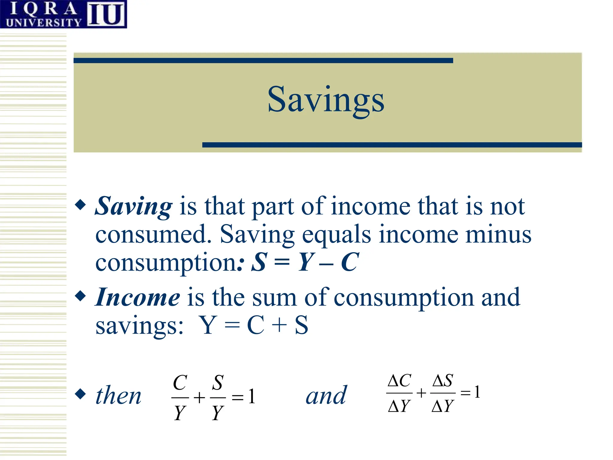
The document discusses key economic concepts such as consumption, savings, and investment. It explains the consumption function and its relationship with income, the marginal propensity to consume, and the concept of savings as the portion of income not spent. Furthermore, it covers the investment multiplier and how changes in investment affect overall output in the economy.

1. Consumption, Savings and
Investment
 Consumption function
 Savings
 The Multiplier

2. Autonomous consumption
 Autonomous consumption expenditure CA
occurs when income levels are zero. Such
consumption does not vary with changes in
income.
 If income levels are actually zero, this
consumption is financed by borrowing or
using up savings.

3. Induced consumption
 Induced consumption CI describes
consumption expenditure by households on
goods and services which varies with
income.
 Consumption is considered induced by
income.

4. Marginal Propensity to
Consume
 The marginal propensity to consume
(MPC) is the extra amount that people
consume when they receive an extra unit of
income.
MPC = ΔC / ΔY
MPC is the first derivation of consumption
function.
 Induced consumption can be described by
formula: CI = MPC . Y

5. The Consumption Function
 The consumption function shows the
relationship between the level of consumption
expenditure and the level of income.
C = f (Y)
If autonomous and induced consumption is
identified then: C = CA + CI
C = CA + MPC . Y

6. The Consumption Function
Y
C
0
Consumption
function C = f(Y)
Savings
Consumption
45˚
Y1 Y 2
CA

7. The Consumption Function
 45˚ line: at any point on the 45˚line
consumption exactly equals income and the
households have zero saving.
 MPC is the slope of the consumption
function, which measures the change in
consumption per unit change in income.

8. Savings
 Saving is that part of income that is not
consumed. Saving equals income minus
consumption: S = Y – C
 Income is the sum of consumption and
savings: Y = C + S
 then and
1


Y
S
Y
C 1






Y
S
Y
C

9. Savings
 The marginal propensity to save
is defined as the fraction of an extra unit of
income that goes to extra saving.
 MPC + MPS = 1 because the part of each
unit of income that is not consumed is
necessarily saved.
Y
S
MPS




10. Saving Function
 Like consumption saving is also the function
of income: S = f(Y)
 If autonomous consumption exists then
autonomous saving exists as well and saving
function is: S = -CA + MPS.Y
 Saving is a source for investment.

11. The Consumption and Saving
Function
Y
C, S
0
C = f(Y)
45˚
Y E
CA
-CA
S = f(Y)
The saving
function is the
mirror image of
the consumption
function. It shows
the relationship
between the level
of saving and
income.

12. The Simple Theory of
Investment
 In the simple Keynesian model,
investment is independent of national
income (autonomous investment).
 The investment function will be a
horizontal straight line.

13. The Investment Function
Y
I
0
I1
In the short-run it
is reasonable to
assume that
investment is
independent of
national income.
I2
I2
I1

14. Consumption and Investment
Functions
 The spending curve shows the level of
desired expenditure by consumers (CA +
MPC.Y) and businesses (I) corresponding
to each level of output.

15. Consumption and Investment
Functions
Y
C, I
0
C = CA + MPC . Y
C + I = CA + MPC . Y + I
I
I

16. Consumption and Investment
Determine Output
 If the level of output is e. g. Y1 at this level
of output the C+I spending line is above
45˚line, so planned spending is greater than
planned output.
 This means that consumers would be buying
more goods than the businesses were
producing. Thus spending disequilibrium
leads to a change in output.

17. Equilibrium National Income
Y
C, I
0
45˚
C + I = CA + MPC . Y + I
E
Y1 YE Y2
Consumption and
investment determine
output

18. Saving and Investment
Determine Output
 Equilibrium occurs when desired saving of
households equals the desired investment of
businesses.
 When desired saving and desired investment
are not equal, output will tent to adjust up or
down.

19. Saving and Investment
Determine Output
Y
S, I
0
S = f (Y)
E
Y1 YE Y2
I
-

20. Saving and Investment
Determine Output
 At output level Y2 families are saving more
than businesses are willing to go on
investing. Firms will have too few
customers and large inventories of unsold
goods than they want. Then, businesses
will cut back production and lay off
workers. This move output gradually
downward and economy returns to
equilibrium YE.

21. Investment Multiplier
 The Keynesian investment multiplier model
shows that an increase in investment will
increase output by a multiplied amount – by
an amount greater than itself.
 The multiplier is the number by which
the change in investment must be
multiplied in order to determine the
resulting change in total output.

22. Investment Multiplier
Y
C, I
0
45˚
C +I1
C + I2
Y1
I2 = I1 + ΔI
ΔY = k . ΔI
Y2
ΔY
ΔI
E1
E2
I
Y
k




23. Investment Multiplier
Y
S
0
S = f (Y)
Y1
I1
-
I2
ΔI
ΔY Y2
E1
E2

24. Investment Multiplier
 The size of the multiplier k depends upon how
large the MPC is.
MPS
MPC
Y
C
C
Y
Y
I
Y
k
1
1
1
1
1














