This document discusses key concepts in the simple Keynesian theory of income determination, including: 1. Endogenous and exogenous variables - endogenous variables are explained by the theory, while exogenous variables are taken as given. Real output and consumption are initially treated as endogenous. 2. The consumption function - consumption is explained as autonomous consumption plus the marginal propensity to consume times disposable income. This can be shown graphically. 3. Induced saving and the marginal propensity to save - as disposable income increases, the remaining portion after consumption is induced saving. Actual U.S. data from 1929-2001 is presented to illustrate these concepts.

1. W,WffiffiWfi rc$
l{inth
Robert J.
rris Professor in the Social SciencesStanley G. Ha
Northwestern University
Ssston Sa,n Frnneisco New York
London Toronto $ydney Tokyo Singapore Madrid
Mexico City Munirh Paris C*pe Town llong Kong Montreal

2. CHAPTER
Endogenous variables are
those explained by an eco-
nomic theory.
Exogenous variables are
those that are relevant but
whose behavior the theory
does not attempt to
explain; their values are
taken as given.
The Simple Keynesian Theory
of Income Determination
Att ltoncsf ttntt is orta utlttt kliozrrs tlnf lu ctttt't cottsrnttc ntorL'tlnrt ltt'ltns Ttrt;tlttct'tl.
-Avn
Rar-rc1, 1c)66
This chapter begins a two-part unit, spanning Chapters 3-8, that develops a the-
ory of business cycles and the potential role of monetary and fiscal policy in
dampening the amplitude of cycles. Our first interest is in fluctuations in real
GDP and interest rates; subsequently we link these fluctuations to the govern-
ment budget, foreign trade, price movements, and inflation.
3-l Business Cycles, Unemployment, and lncome
Determination
In section 2-70 you learned that fluctuations in unemployment are the mirror
image of fluctuations in output or, more precisely, in the difference (gup)
between actual and natural real CDP. When that gap rises into positive territory
as the economy expands, the unemployment rate falls; when that gap becomes
negative as the economy slides into a recession, the unemployment rate rises.
Thus thekey to tmderstnnding the causes offluctttations in unemployment is to deuelop
a theory of fluctuntions in resl CDP.
What We Explain and What We Take as Given
Any theoretical model in economics sets limits on what it tries to explain. The
limited number of variables to be explained are called endogenous variables.
The large number of variables that are taken as given and are not explained are
called exogenous variables.
In macroeconomic theory we begin with a short list of endogenous vari-
ables and treat most as exogenous. Gradually, we move some from the exoge-
nous list to the endogenous list as our theory becomes more realistic. Table 3-1
shows the major variables that we analyze and their status as endogenous or
exogenous.
This list excludes some variables that are treated as exogenous throughout,
especially the money supply, the level of government spending, and tax rates.
Although not included in the list, other exogenous elements, sometimes called
61

3. (i2 THI.l SIIlf)l.E IiEYNF,SI'N 'f Hli()li- oI I('()Iill I)i)f iiRllIA'l'i()-i
3-1 Endogenous and Exogenous Variables in the Theory
of Business Cvcles
r-'
-- -t
I
-i
Chapter 3
Chapte'r 4
l, nclogcrt orrs
Real output
Consumption
Price le,u'el
Real outpr,rt
Consumption
Investment
Lrterest rate
Real output
Consr-rmption
Investment
Interest rate
Price level
F)rog'rn itrr s
Investment
Interest rate
Price level
Chapter 7
tJt'nuutd shocks, are some of the basic causes of business cycles; they include the
effects of wars and other political crises, and unpredictable changes in spending
on consumption, investment spending, ancl net exports. Finally, other exoge-
nous variables, supply shocks, include major changes in the price of oil or other
raw nraterials.
Lc'ar,,ing aside these excluded exogenous varial'rles, we see from Table 3-1
that our theory develops one element at a time, successively movir'rg variables
frorn the exogenous to the endogenous category. We begin in the next section
with a simple theory that explains consumption and real output, treating invest-
ment, the interest rate, and the price level as exogenous.
3-2 PlannedExpenditure
Our study of national income accounting in Chapter 2 identified four types of
expenditure on CDP. By definition, total expencliture orl GDP (E ) is equal to the
sum of these four components: consumption (C), investment (I), government
spending on goods and services (C), arrd net exports (NX).
E:C+IIC+NX (3.i)
The Consumption Function
At the beginning, we treat only consLlmption spending (O as endogenous, or
explained by the theory, and treat the other three types of plannecl spending as
exogenous. An obvious way to explairr consumption is that people spend more
when their incomes go up and vice versa. The income that matters for con-
sumption decisions is income after taxes, or disposable personal income. This
can be written as total real incom e (Y) minus personal taxes paicl (T), or Y - T.r
1'Ihe rrotatjon T in this ch.lpter continues, ;rs in Chapter 2, to mean "total taxes mintrs transfer
payments."

4. t],)
An autonomous magni-
tude is independent of the
level of income.
The marginal propensity
to consume is the dollar
change in consumption
expenditures per dollar
change in disposable
income.
Induced consumption is
the portion of consump-
tion spending that
responds to changes in
income.
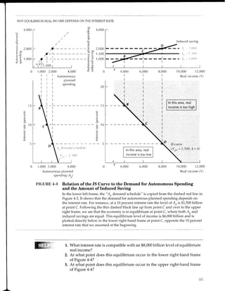
How do households divide their disposable income between consumption
and saving? Households consume a fixed amount that does not depend on their
disposable income, plus a fraction of each dollar of disposable income:
(,r'nr'r',il I int'.rr iorn
C: Co + ,U -;; (3.2)
The fixed amount is called autonomous consumption, abbreviated (Cr), and
this is completely independent of disposable income. The amount by which
consumption expenditures increase for each extra dollar of disposable income
is a fraction called the marginal propensity to consume, abbreviated (c). This
equation (3.2) says in words that consumption spending (C) equals autonomous
consumption (C) plus the marginal propensity to consume times disposable
income lc(Y - T)]. Another name for this last term is induced consumption.
The consumptionfunction is any relationship that describes the determinants
of consumption spending. This function can be written as a general expression,
as in equation (3.2), or as a numerical example. For instance, if we choose $500
billion to be the value of autonomous consumption and 0.75 to be the value of
the marginal propensity to consume, the consumption function can be written
ttrtrt't'ic,ti I r.trrr;,lt'
C:500+0.75(Y-T)
Either way of writing the consumption function, either in the general version of
equation (3.2) or in the specific numerical example, states that total consump-
tion is the sum of autonomous consumption and induced consumption.
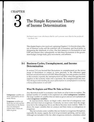
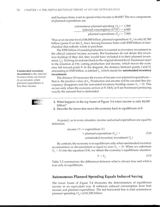
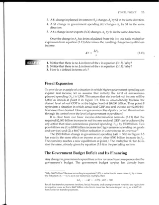
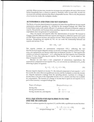
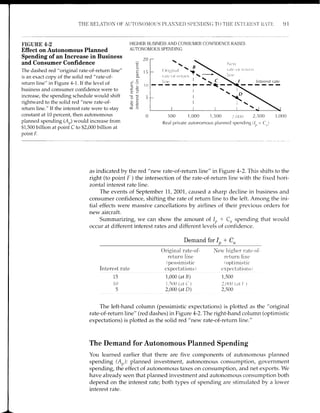
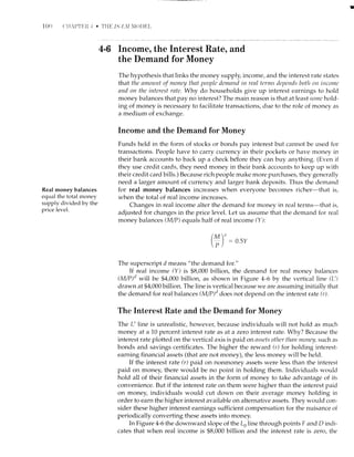
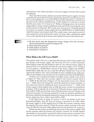
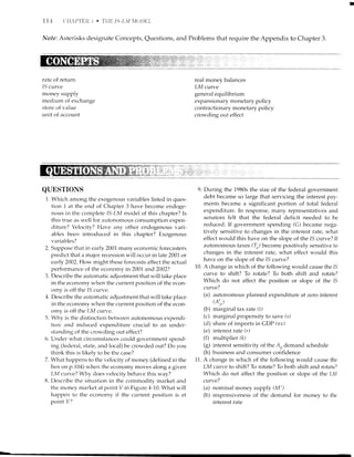
The consumption function can also be shown graphically, as in Figure
3-1. The thick red line shows on the vertical axis the amount of consumption for
alternative values of disposable income (measured along the horizontal axis).
When disposable income is zero, total consumption consists just of the
autonomous component ($5OO billion). For each extra $1,000 billion of dispos-
able income, as we move to the right on the graph, the red consumption func-
tion line rises by $750 billion, since its slope (the marginal propensity to
consume) is 0.75. For instance, at point D disposable income is $8,000 billion and
total consumption is $6,500 billion (consisting of $6,000 billion of induced con-
sumption and $500 billion of autonomous consumption).
L. If a person's disposable income is zero, what is that person's level of con-
sumption spending in the general linear form of equation (3.2)? In the
numerical example?
2. How can that person consume a positive amount with a zero disposable
income? Think of yourself-what options are open to you to buy some-
thing even if you had no income?
Induced Saving and the Marginal Propensity to Save
The simplest way to show the amount of saving is to use a graph like Figure 3-1.
The thick black line shows the amount of disposable income in both a horizon-
tal and a vertical direction; this line is often called the "45-degree" line. Since the
thick red line shows the consumption function, the distance between the two
lines indicates the total amount of saving.

5. 64 (.}]APTF]R :J . TFIE SIIPL}.] KIIYNESIAN THEORY OF'INI]f)T{!] DETERNIINATIC)N
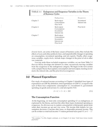
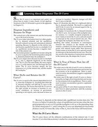
FIGURI' 3.1
A Simple Hypothesis Regarding
Consumption Behavior
The red line passing through F and D
illustrates the consumption function. It shows
that consumption is 75 percent of disposable
income pltrs an autonomous conlponent of
$500 billion that is spent regardless of the
lerrel of disposable income. The red sl-raded
area shows tire amount of positive saving that
occurs when income exceeds consumption;
the grav area shows the arnount of negative
saving (dissaving) that occurs when
consumption exceeds income.
HOW DISPOSABLE INCOME IS DIVIDED BETWEEN CONSUMPTION
AND SAVING
10,00t)
8,000
6,500
6,000
4,000
2,000 4,000 6,000 8,000 I0,000
Real disposable income (Y-f)
U
q)
=.=
7,
c
o_
X
C
o.F
o_
E
f
C
o
G
CJ
u
I---l rotal
l----l total s.rving negative
Disposable income
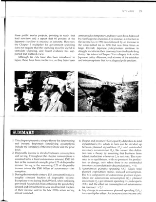
To the right of point F, total saving is positive because disposable income
exceeds consumprtion; this is indicated by the red shading. To the left of point F,
total saving is negative because consumption exceeds disposable income; this is
indicated by the gray shading. How can sarring be negative? Individuals can
consume more tl-ran they earn, at least for a while, by withdrawing funds fron-r
a savings account, by selling stocks and bonds, or by borrowing. Negative sav-
ing is quite typical for many students who borrow to finance tl-reir education.
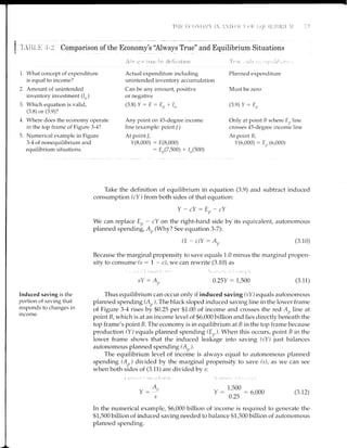
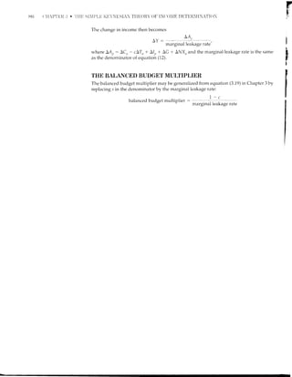
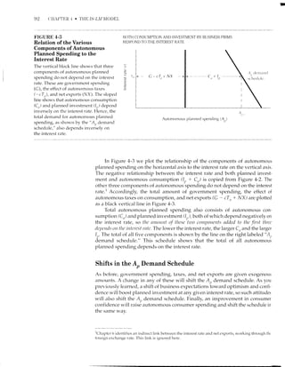
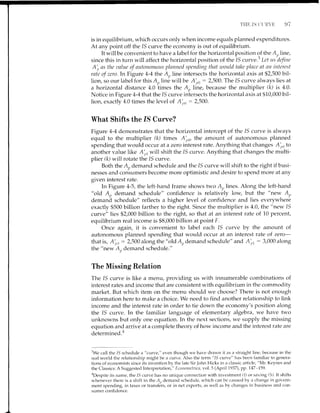
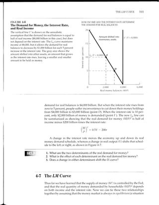
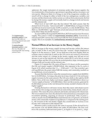
Figure 3-2 illustrates the relationship between induced saving, autono-
mous consumption, and total saving. The top frame duplicates Figure 3-1 but
highlights the division of disposable income between induced consumption
[0.75(Y - T)] and induced saving [0.25U - T)]. The bottom frame subtracts
induced consumption from the top frame and isolates the relationship between
autonomolrs consumption and induced saving.
The shaded rrertical distance between the black and red lines represents sav-
ing (S), that is, the difference between disposable income and consumption:
Ct,rrcr.rl Linear Frttrm
S: Y-T-C: Y-T-Cn-c(Y-T) 5
: -Cu + 0. - c)(Y -T) (3.3)
This sazring fiutction starts with the definition of saving as personal disposable
income minus consulnption; then it substitutes the consumptior-r function from
equatiorl (3.2). The last line simplifies the saving fur-rction, which now states that
N r,r nrt'ric.r I Era ur ple
- Y-T-C: Y-T-500 -0.75U-T)
: -500 + 0.25(y -T)

6. PLANN]jD iiX PIN t)t'l't. titi 6ir
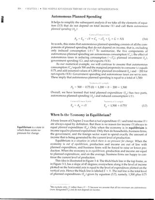
FIGURE 3.2
The Relation Between Induced
Consumption, Induced Saving, and
the Consumption Function
The upper frame duplicates Figure 3-1. The
thin black line shows the dividing line
between induced saving and induced
consumption. Starting at zero disposable
income, each dollar of disposabie income is
divided between 75 cents of induced
consumption and 25 cents of induced
saving. The lower frame subtracts induced
consumption from the upper frame. It
shows the relation between induced saving
and autonomous consumption. Total
saving in both parts of the diagram is
shown by the red and gray shading and
equals induced saving minus autonomous
consumption.
ANY CHANGE IN DISPOSABLE INCOME IS DIVIDED BETWEEN
INDUCED CONSUMPTION AND INDUCED SAVING
lnduced
savi ng
= 0.25 (Y-T)
lnduced
consumption
= 0.75 (Y_T)
2,000 4,000 6,000 8,000 10,000
Real disposable income (Y-f)
2,000 4,000 5,000 8,000 10,000
Real disposable income (Y-f)
Induced
saving
= 0.25 (Y-T)
Marginal propensity to
save is the change in
personal saving induced
by a $1 change in personal
disposable income.
personal saving equals minus the amount of autonomous consumption (-C,r)
plus the marginal propensity to save (7 - c) times disposable income U - T).
Notice the three points in both frames of Figure 3-2 marked with letters cor-
responding to different levels of disposable income. At H, disposable income is
zero, so consumption is C,,, or 500, and saving from equation (3.3) is -Cn, or
-500. AtF, disposable income and consumption are equal, so saving is zero. At
D, consumption of 6,500 is less than disposable income of 8,000, so saving is a
positive 1,500.
ffiN$ 1,.
2.
Can you derive a general expression showing how the level of consump-
tion and disposable income at point F depend on autonomous consump-
tion (Co) and the marginal propensity to consume (c)?
If disposable income is 5,000 rather than 8,000, the economy in Figure
3-2 will be at a point between points F and D. Calculate the values of con-
sumption (C) and saving (5) when disposable income is 5,000.

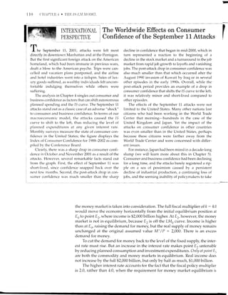
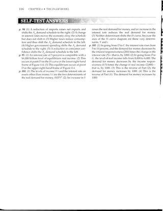
7. (i6
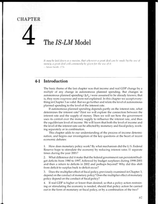
Wuv Drn U"S. Savmc Alnnosr VaNrsH rN 2001?
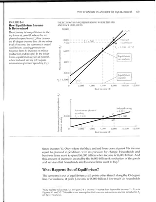
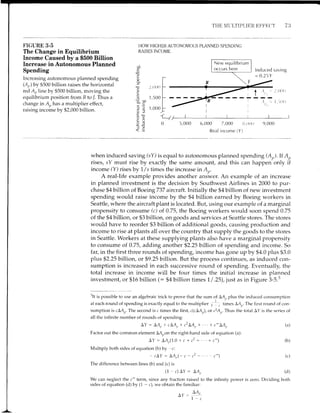
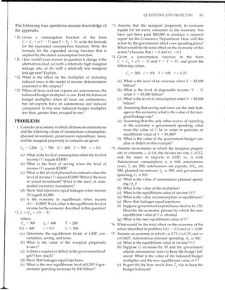
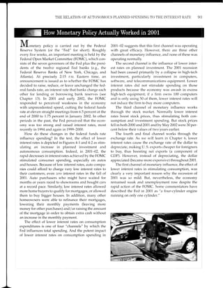
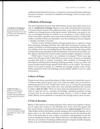
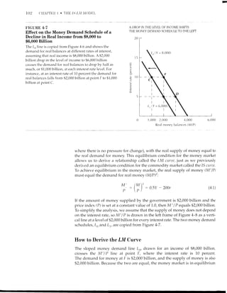
Figure 3-3 is arranged exactly like Figure 3-1 and shows the actual values of dis-
posable income and consumption spending in the United States during the
years 7929-2001. As in Figure 3-1, the amount of personal saving' is shown by
the light red shaded area between the black and red lines.
Four major conclusions can be drawn from the evidence. First, consumption
increased as disposable income grew during the years since World War II.
Second, in the worst years of the Great Depression, in 7932 and 1933, house-
holds consumed more than their entire disposable incomes, so the fraction
saved was negative (-0.9 percent in7932 and -1.5 percent in 1933). Third, these
usual peacetime relationships were interrupted during World War II (794215),
when consumer goods were unavailable or rationed. In that period, households
F-[(;URII 3-:i
Consumption, Saving,
and Disposable
Income, 1929-2001
In 2001 saving was bareiy
positive and amounted to
a mere 1.6 percent of
disposable income. Saving
was unusualiy high cluring
World War II because
consumer goods were
rationed. During the four
decades before 2001,
personal saving as a
percentage of disposable
income ranged from 5.3 to
9.7 percent.
HOW ACTUAL U.S. DISPOSABLE INCOME HAS BEEN SPLIT
BETWEEN CONSUMPTION AND SAVING
8,000
=--o
O)
O)
o
C
::o
.F
o-
E
C
?
M.
7,OOO
6,000
5,000
4,0O0
3,000
2,O00
'1,000
0
[_-] Area inclicates disposable
income minus consumption,
or personal s.rving
t1929
1 933
1,000 2,000 3,000 4,000 5,000 6,000 7 ,oo0 8,000
Real disposable income (billions of 1996 clollars)
World War ll
saving bulge
'Be careful to distinguish between "savings" (with a terminal "s"), which is the stock of assets that
households have in savings accounts or under the mattress, from "savrng" (rvithout a terminal "s"),
which is thefTozr per unit of time that leaks out of disposable income and is unavailable for pur-
clrases of consumption goods. It is the flow of sauittg that is designatecl by the symbol S.

8. THE ECONON'IY IN AND OI,IT (X' EOIIII-IBRII]II 67
were forced to consume much less and save much more than is normal in peace-
time, fully 26 percent of disposable income tn7944. After the war, consumers
rushed out to spend their accumulated savings, helping to maintain prosperity.
The fourth conclusion is quite surprising. In the late 1980s and throughout
the 1990s, real personal saving decreased, from about 9447 billion in79}4,to$272
billion in7996, to a mere $121 billion in 2001. The gradual shrinking of saving in
the 1990s was generally attributed to the long stock market boom following 1982,
during which the average value of stock prices increased tenfold. Consumers
were able to raise their consumption relative to their disposable income by sell-
ing some of their stocks that had enjoyed large capital gains. Also, consumers
were able to boost their consumption by taking advantage of lower interest rates
and refinancing their home mortgages. In Chapters 4 and 15 we return to the
influence of interest rates and stock prices on consumption behavior.
3-4 The Economy In and Out of Equilibrium
Until now we have seen that the level of consumption spending depends on
disposable income. But so far we have no idea what the level of income will
actually be. $5,000 billion? $10,000 billion? We need an extra element, besides
the consumption function, to construct our theory of income determination.
This extra element is that expenditure is not always what is desired or
planned, and if some expenditure is unplanned, business firms will adjust pro-
duction until the unplanned component of expenditure is eliminated. The total
amount of spending that people want to do includes only the planned compo-
nent, called planned expenditure (Ep). The rest of expenditwe (E - Er,) is
unplanned and undesired. To simplify, we assume that investment (I) is the bnly
component of total expenditure that can contain an unplanned component,
whereas consumption (C), government spending (G), and net exports (I,JX) are
akuays equal to the planned ctmount.
Er:C+Ip+G+l/X
The four components of expenditure are exactly the same as in equation (3.1),
except that we use a subscript "p" for investment, since only for that component
of expenditure do we need to distinguish between the planned amount (lr,) and
the unplanned amount (1,,).
The next step is to combine the consumption function from equation (3.2)
with the definition of planned expenditure from equation (3.a):
Er,: Cn + c(Y - T) + It) + G +
^/x
(3.4)
(3.s)
A parameter is a value
taken as given or known
r.t'ithin a particular
analvsis.
In words, this states that planned expenditure equals autonomous consump-
tion, plus the part of consumption that depends on disposable income (induced
consumption), plus the fixed values of planned investment, government spend-
ing, and net exports.
The word parameter means something that is taken as given, including not
only exogenous variables but also fixed elements of a function. In the case of the
consumption function, there are two such fixed elements (Co and c), andwe will
take both as given. In addition, the three components of planned expenditure
other than consumption (1r,, G, and NX) can be considered as both exogenous
variables and parameters.

9. tis
ffi
Autonomous Planned Spending
It helps to simplify the subsequent anaiysis if we take all the elements of equa-
tion (3.5) that do not depend on total income (Y) and call them sutonontous
plnnned spending ( A,,, ):
( ,t'nt'r'al I inr'.l l ()l nt
Ap: E, - cY : Cn - cTn + Ip + G + l/X
In words, this states that autonomous planned spending consists of all the com-
ponents of planned spending that do not depend on income, that is, excluding
only induced consumption (cY).3 To summarize, the five components of
autonomous planned spending are autonomous consumption (C,r), the effect of
autonomous taxes in reducing consumption (-cTn), planned investment 0,,),
government spending (C), and net exports (l/X).
As our numerical example, we will continue to assume that autonomous
consumPtton(C) equals 500 and the marginal propensity to consume (c) equals
0.75, and add assumed values of 7,200 for planned investment (Ir) and -200 for
net exports (NX). Government spending and autonomous taxed are set to zero.
These imply that autonomous planned spending is equal to a total of 1,500:
rrrrr,'r'i,,rl i .,,rirr1'1,.
At, : 500 - 0.75 (0) + 7,200 + 0 - 200 : 1,500
Overall, we have learned that totai planned expenditure (Er,) has two parts,
autonomous planned spending (Ar) and induced consumption (cy).
( ,r'nr't',t I I-irrt'.t r l:orrlr
Er: A, + cY
ttittclir.rl i r,tntl-rli'
E,,: 7,500 + 0.75Y
(3 6)
(3.7)
Equilibrium is a state in
which there exists no
pressure for change.
When Is the Hconomy in Bquilibrium?
A basic lesson of Chapte r 2 w as that actual expendi ture (E ) and total income (y )
are always equal by definition. But there is no reason for income (Y)always to
equal plnnned expenditure (Er). Only when the economy is in equilibrium is
income equal to planned expenditure. Only then do households, business firms,
the government, and the foreign sector want to spend exactly the amount of
income that is being generated by the current level of production.
Equilibrium is a situation in uthich there is no pressure for change. When the
economy is out of equilibrium, production and income are out of line with
planned expenditure, and business firms will be forced to raise or lower pro-
duction. When the economy is in equilibrium, production and income are equal
to planned expenditure, and on the average, business firms are happy to con-
tinue the current level of production.
This idea is illustrated in Figure 3-4. The thick black line in the top frame, as
in Figure 3-3, has a slope of 45 degrees; everywhere along it the level of income
plotted on the horizontal axis is equal to the level of expenditure plotted on the
vertical axis. Hence the black line is labeled E : Y. The red line is the totai level
of planned expenditures (E,,) given by equation (3.7), namely, 1,500 plus 0.25
rWe exclude only cY rather than c(Y - l") because we assume that all tax revenues are autonomous
(now designated Ir) and do not depend on income.

10. THE EOONONTY IN AND OUT OF EQUILIBRIT-INI 69
FIGURE 3.4
How Equilibrium Income
Is Determined
The ecottcrmv is in equilibrium in tl're
top frame at point B, where the red
planned expenditure (E,,) line crosses
the,lS-c-legrce income line. At any other
level of income, the economy is out of
equilibrium, causing pressure on
L-rusiness firms to increase ol reduce
production ancl income. ln the lower
frame, equilibrium occurs art point B,
rvhere inducecl saving (sY) equals
autonomous plernned spencling (4,,).
THE ECONOMY IS IN EQUILIBRIUM ONLYWHERETHE RED
AND BLACK LINES CROSS
10,000
8,000
7,500
6,000
'+,00t)
2,000
2,00t) 4,000 (),(X)0
Real inconre
t
A = 1.500 {
r' I
o
0,
=.=-o
C
c)
o_
X
.J
-(,
O
C
c
c-
CJ
l
-=
-o
C
a)
c_
X
a,
-a
c
c
*c
f,>
c-
tr=
<':
8,000 -l0,000 12,000
4,Ot)O (r,000 8,000 10,000 12,00(l
Real incomc (Y)
lnducecl saving,
times income (Y). Only where the black and red lines cross at point B is income
equal to planned expenditure, with no pressure for change. Householcls and
business firms /ant to spend $6,000 billion when income is $6,000 billion. And
this amount of income is created by the $6,000 billion of production of the goods
and services that householcls and business finns wallt to buy.*
What Happens Out of Equilibrium?
The economy is out of equilibrium at all points other than B along the 45-clegree
line. For instance, at point /, income is $8,000 billion. How much do households
4Note that the horizontal axis in Figure 3-4 is income (Y) rather than clisposable income (Y - T) as irr
Figr-rres 3-1 atrd 3-2. This reflects our assumption that taxes are arttot-totttous .lt-Id are iuclttdec-l in 4,,
on thc' r,erticirl axis.

11. 70 (IHAPTER ll . 'fIIE SIN'IPL11 KEYNFISIAN THllOIi'f)F IN('OIIE IlliTFlt'illtN.l'l()
and business firms want to spend when incotne is $8,000? The two components
of planned expenditure are:
autonomous planned spending (A,,) : 1,500
induced consLunption (0.75Y ) : 6,000
Unintended inventory
investment is the amount
btisiness firms are forced
to accun'rttlate when
planned expenditr,rre is
less than income.
planned expenditure (Er) -- 7,500
Thtrs at an income level of $8,000 billion, planned expendit:u.re (Et) is only $2500
billion (point H on the E,, line), leaving business firms with $500 billion of mer-
chandise that nobody wAnts to purchase.
The $500 billion of unsold production is counted as inventory investment in
the official national income accoullts. But businesses do not desire this inr,'en-
tory buildup (if they did, they would have included it in their planned invest-
ment,1,,). To bring inventories back to the original desired level, businesses react
to the dituation at I by cutting production and income, which moves the econ-
omy left toward point B. In the diagram, the distance between points I and H,
amounting to $500 billion, is labeled 1,,, which stands for unintended inventory
investment.
The distance /H measures the excess of income over planned expenditure-
that is, the positive'n,alue of /,,. Production and income will be cut until this dis-
crepancy disappears and the unwanted inventory buildup ceases (1,,: 0). This
occurs only when the economy arrives at B. Only at B are businesses producing
exactly the amount that is demanded.
1. What happens in the top frame of Figure 3-4 when income is only $4,000
billion?
2. Describe the forces that move the economy back to equilibrium at B.
At point /, as in every situation, income and actual expenditttre are equal by
definition:
income (Y) = expenditure (E)
: planned expenditure (Er,) +
unintended inrrentory investment (1,, )
By contrast, the economy is in equilibrium only when unintended inventory
acctrmulation or decumulation is equal to zero (1,,-- 0). When we substitute
(1,, -- 0) into the equation (3.8), we obtain the economy's equilibrium situation:
(3 B)
(3.e)Y:l-
t,
Table 3-2 summarizes the differences between what is always true and what is
true only in equilibrium.
Autonomous Planned Spending Equals Induced Saving
The lower frarne of Figure 3-4 illustrates the determination of equilibrium
income in an equivalent way. It subtracts induced consttmption from both
income and plannecl expenditure. The red horizontal line is total autonomous
planned spending (A,,) of $1,500 billion.

12. t^
IIg!
s
Comparison of the Economy's 'Always True" and Equilibrium Situations
A;it ri., s ll ur, ii..' illii;tiliritl
Actual expenditure including
unintended inventory accumulation
Can be any amount, positive
or negative
(3.8) Y:E:Eu*1,,
Any point on 45-degree income
line (example: point / )
At point /,
Y(8,000) : E(8,000)
: Er,(7,500) + Ir,(5oo)
i't'i r, , ,ii ii r
2.
J.
What concept of expenditure
is equal to income?
Amount of unintended
inventory investment (I,, )
Which equation is valid,
(3.8) or (3.9)?
Where does the economy operate
in the top frame of Figure 3-4?
Numerical example in Figure
3-4 of nonequilibrium and
eqtrilibrium situa tions.
Planned expenditure
Must be zero
(3.9) Y : E,,
Only at point B where E,, line
crosses 45-degree income line
At point B,
Y(6,000) : Er, (6,000)
Take the definition of equilibrium in equation (3.9) and subtract induced
consumption (cY) from both sides of that equation:
Y-cY--Et)-cY
We can replace Ep - cY on the right-hand side by its equivalent, autonomous
planned spending, Ar, (Why? See equation 3-7):
(7-c)Y:At,
Because the marginal propensity to save equals 1.0 minus the marginal propen-
sity to consume (s : 1 - c), we can rewrite (3.10) as
(3.10)
(3.11)
(3.12)
sY:4,
Thus equilibrium can occur only if induced saving (sY) equals autonomous
planned spending (Au ). The black sloped induced saving line in the lower frame
of Figure 3-4 rises by $0.25 per $1.00 of income and crosses the red A,, line at
point B, which is at an income level of $6,000 billion and lies directly beneath the
top frame's point B. The economy is in equilibrium at B in the top frame because
production (Y) equals planned spending (Ep). When this occurs, point B in the
lower frame shows that the induced leakage into saving (sY) just balances
autonomous planned spending (A, ).
The equilibrium level of income is always equal to autonomous planned
spending (Ar,) divided by the marginal propensity to save (s), as we can see
when both sides of (3.11) are divided by s:
(,('rt{'1,,1 I ril,.',ri I l|.itl
t1.,,
/_ r
I-
s
In the numerical example, $6,000 billion of income is required to generate the
$1,500 billion of induced saving needed to balance $1,500 billion of autonomous
planned spending.
'..::1,, l j.. .l l ..,ri,l;, .
0.25Y : 1,500
lnduced saving is the
portion of saving that
responds to changes in
income.
":';:rT:6,ooo

13. 72 C]HAP'fER I] . THE SI,{PLE K!]YNESIAN THEORY OF INCOIE DETERX'iINATION
3-5 The Multiplier Effect
Our conclusion thus far that equilibrium income equals $6,000 billion is
absolutely dependent on our assumption that autonomous planned spending
(Ar,) equals $1,500 billion. Any change in autonomous planned spending will
cairse a change in equilibrium income. To illustrate the consequences of a change
in A., we shall assume that business firms become more optimistic, raising their
g.t"dr as to the likely profitability of new investment projects. They increase their
investment spending by $500 billion, boosting Ao from $1,500 billion to $2,000
billion. In each situation where a change is described, a numbered subscript is
used to distinguish the original from the new situation. Thus 4o6 denotes the orig-
inal level of A, ($1,500 billion), and A4 denotes the new level ($2,000 billion).
Calculating the Multiplier
We can use (3.12) to calculate the equilibrium level of income in the new and old
situations. Note that only A,, changes; there is no change in the marginal Propen-
sity to save (s).
(,1'tl('l'.11 I itlt',ll Iittl'tll N r-r nrclic.r I F ra rtrp it'
2,000
Y,:; ^- : 8,000- u./-3
1,500
Y' : iru
: 6'ooo
Take new situation Y1 --
Subtract old situation Y,, :
A
^p7
s
4q
s
The multiplier is the ratio
of the change in output to
the change in autonomous
planned spending that
causes it. It is also 1.0
divided by the marginal
propensity to save.
(,t'rlet.ai I-tttc.lt' lrot rtt
AY 1
multiplier (k) : :
LAt, s
Equais change in income
multiplier (k)
AY:#:2,ooo (3.13)
AA,,
AY: -r
s
The top line of the table calculates the new level of income when A7,1rs at
the new value of 2,000. The second line calculates the original level of income
when,4,,,, is at the old value of 1,500. The change in income, abbreviated AY, is
simply the first line minus the second. The multiplier (k) is defined as the ratio
of the change in income (LY) to the change in planned autonomous spending
(LA) that causes it:
Lr nit't'ica I l:x.t rrr ;r ie
Ar: 1 :4.0
LAr, 0.25
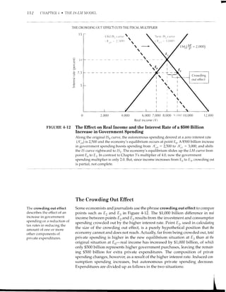
In Figure 3-5 we can see why the multiplier (k) is 7f s, or 4.0. Figure 3-5
reproduces from Figure 3-4 the original situation, with A, at its original value of
$1,500 billion.
The 9500 billion increase in A,causes the A,, line to shift upward by $500 bil-
lion and to intersect the fixed induced saving line at point /. Because only 25 per-
cent of extra income is saved, income must rise by $2,000 billion to generate the
required $500 billion increase in induced saving. In terms of the line segments:
R/ 1.. RB,
RB: s(slnces: Rl)
Example of the Multiplier Effect in Action
How does the magic of the multiplier work? One answer is given by Figure
3-5, which is based on the idea that the economy can be in equilibrium only
(3.14)

14. THE NILILTIPLIETi Ii F'F'F,(I'I'
rJ t)
t,)
FIGURE 3-5
The Change in Equilibrium
Income Caused by a $SOO Billion
Increase in Autonomous Planned
Spending
Increasing autonomous planned spending
(At) by $500 billion raises the horizontal
red Ar line by $500 billion, moving the
equilibrium position from B to /. Thus a
change in A, has a multiplier effect,
raising income by $2,000 billion.
HOW HIGHE,R AUTONOMOUS PLANNED SPENDING
RAISES INCOME
,,,,,,,,
f1,s00
l-
1,O00,
.g
c
o_
c
c
_C
f>
-(!
v d)
c-
YJ
{-1 t l r r t
5,000 6,000 7,OOO il.()0o
Real income (Y)
9,000
Induced saving
= 0.25Y
when induced saving (sY) is equal to autonomous planned spending (A).If At:,
rises, sY must rise by exactly the same amount, and this can happen'only if
income (Y) rises by 7 / s times the increase in A,,.
A real-life example provides another answer. An example of an increase
in planned investment is the decision by Southwest Airlines in 2000 to pur-
chase $4 billion of Boeing 737 airuaft. Initially the $4 billion of new investment
spending would raise income by the $4 billion earned by Boeing workers in
Seattle, where the aircraft plant is located. But, using our example of a marginal
propensity to consume (c) of 0.75, the Boeing workers would soon spend 0.75
of the $4 billion, or $3 billion, on goods and services at Seattle stores. The stores
would have to reorder $3 billion of additional goods, causing production and
income to rise at plants all over the country that supply the goods to the stores
in Seattle. Workers at these supplying plants also have a marginal propensity
to consume of 0.75, adding another $2.25 billion of spending and income. So
far, in the first three rounds of spending, income has gone up by $4.0 plus $3.0
plus $2.25 billion, or $9.25 billion. But the process continues, as induced con-
sumption is increased in each successive round of spending. Eventually, the
total increase in income will be four times the initial increase in planned
investment, or $16 billion (: $4 billion times 7/.25),just as in Figure 3-5.)
'It is possible to use an algebraic trick to prove that the sum of A1,, plus the inclr.rcecl consumption
at each round of spending is exactly equal to the multiplier pi times AA,,. The first rouncl of con-
sumption is cAA,,. The second is c times the first, c(cLAr), or c2A,,. Thus the total AY is the series of
all the infinite number of rounds of spending:
L,Y : L,A,, + cLA,, + c2L,A,,+ .. . + c-AA,,
Factor out the common element AA,,on the right-hand side of equation (a):
AY : AA,,(1.0 + c + c2 +"' + c-)
Multiply both sides of equation (b) by ci
- cAY: AA,,(- c - cl -... c-)
The difference between lines (b) and (c) is
(1 - c) AY : AA,,
We can neglect the c- term, since any fraction raised to the infinity power is zero
sides of equation (d) by (7 - c), we obtain the familiar:
AA,,
AY: '
1-c
(a)
(b)
(c)
(d)
Dividing both

15. ;i
3-G Fiscal Policv
Is a multiplier J*Ounrtnn or contraction of output following a change in
autonomous planned spending desirable or not?
Assume that the desired level of real CDP is $8,000 billion. In Figure 3-5, a
level of autonomous planned spending (Ar,) of $2,000 billion would be perfect,
for it would bring about an equilibrium level of actual real GDP of $8,000 billion
at point /, the desired level. On the other hand, a decline in A, by $500 billion
would cut equilibrium income to $6,000 billion at B and would open up a gap
of $2,000 billion between sctunl and the desired level of real CDP.
What might calrse actual real CDP to decline below the desired level? A
drop in planned investment, a major component of Ar,, car. be and has been a
major cause of actual real-world recessions and depressions. In the Creat
Depression, for instance, fixed inrzestment dropped by 81 percent, and this con-
tributed to the 27 percent decline in actual real GDP between 7929 and7933.
Government Spending and Taxation
The government can adjust its expenditures on goods and services as well as its
tax revenues in an attempt to offset fluctuations in real GDP caused by move-
ments in autonomous consumption, in planned investment, and in net exports.
Our definition of autonomous planned spending (Ar,) rn equation (3.6) already
includes government sprending (G) and the effect of autonomous taxes (T,r) on
consumption. For convenience we repeat equation (3.6):
(
't'ttt'r'.tl I irtr'.tt' l ot'tt'i
Ar,: cn- cTu+ lr,+ G + l'Ix (3.6)
1". Why is 1, written with a p subscript, but the other components of autono-
mous planned spending (Co, - cT* C, and NX) are not?
2. Why does the (cf) term appear with a minus sign but all the other sums
appear with a plus sign?
Equation (3.6) states that autonomous planned spending equals the sum of five
components. It also implies that the chnnge in autonomous planned spending
equals the sum of the clnnge in each of the same five components. We can state
this idea as an equation if we insert the "change in" symbol, A, in front of each
element in equation (3.6). The only remaining element without a A symbol is the
marginal propensity to consume (c), which we are assuming to be fixed
througirout this discussion:
LA, -- ACn - cAf + A1,, + AC + Al/X
ln sum, the five causes of changes in A,, are:
1. A $1 change in autonomous consumption (Cn) changes A,,by $1 in the same
direction
2. A $1 change in autonomolrs tax revenue (7,,,) changes Arby c (the marginal
propensity to consume) tirnes $1 in the opposite direction.
(3.15)

16. F'ISCAL POLICY 7 l-t
3. A$1 change inplanned investment(Ir,) changes A,by $1 in the same direction.
4. A $1 change in government spending (G) changes A, by $1 in the same
net exports (l/X) changes Auby $1 in the same direction.
Once the change in Arhas been calculated from this list, our basic multiplier
expression from equation (3.13) determines the resulting change in equilibrium
income:
direction.
5. A $1 change in
LA,.
AY: t'
s
(3.13)
1. Notice that there is no A in front of the c in equation (3.15). Why?
2. Notice that there is no A in front of the s in equation (3.13). Why?
3. How is s defined in terms of c?
Fiscal Expansion
To provide an example of a situation in which higher government spending can
expand real income, let us assume that initially the level of autonomous
planned spending (A,,) is 1,500. This means that the level of real income will be
6,000, as shown at point B in Figure 3-5. This is unsatisfactory, because the
desired level of real CDP is at the higher level of $8,000 billion. Thus point B
represents a situation in which actual real GDP and real income are $2,000 bil-
lion lower than desired. How can government fiscal policy correct this situation
through its control over the level of government expenditure?
It is clear from our basic income-determination formula (3.13) that the
required $2,000 billion increase in real income and real GDP can be achieved by
any action that raises autonomous planned spendrng (Ar) by $500 billion. TWo
possibilities are (1) a $500 billion increase in G (government spending on goods
and services) and (2) a $667 billion reduction in autonomous tax revenue.o
The $500 billion change in government spending (AC : 500) in Figure 3-5
has exactly the same effect on income as any other $500 billion increase in A,,.
The economy reaches a new equilibrium at point /. The multiplier (k) for AG is
also the same, already given by equation (3.14) in the preceding section.
The Government Budget Deficit and Its Financing
Any change in government expenditure or tax revenue has consequences for the
government's budget. The government budget surplus has already been
nwhy
$667 billion? Because according to equation (3.15), a reduction in taxes raises A,,by c times
the reduction. If c : 0.75, as in our numerical example, then
LAt,- c AT: -0.75(-667) : 500
Recall that transfer payments (welfare, Social Security, and unemployment benefits) are equivalent
to negative taxes, so that a $667 billion reductiort in taxes has the same impact on A,, as a $667 bil-
lion increase in transfer pavments.

17. 76 CHAPTER i] . THE SIMPLE KEYNESIAN THEORY OF INCOI'IE DETERNIINATION
defined in Section 2-4 as tax revenue minus government expenditure (T - G),
which in turn equals investment plus net exports minus private saving.'
T-C=1+l/X-S
Similarly, the change in the left side of the equation must balance the change in
the right side:
AT-AC-A/-Al/X-AS (3.16)
When the government boosts its spending by 500, the movement in Figure
3-5 from point B to point / assumes that autonomoLrs consumption, investment,
and net exports are fixed (ACu : A1 : Al/X : 0) and that tax revenue remains
at zero (AT : 0). Thus the only elements of (3.16) that are changing are AS and
AC. The value of AG is the fiscal stimulus of 500. But what is the value of AS?
Recall from the saving function shown in equation (3.3) that saving changes by
the marginal propensity to save times the change in disposable income,
AS : r^(AY - AT). Using this expression for saving, we can substitute the num-
bers for this example into equation (3.16) and obtain:
AT - AC : AI + Al/X - s(AY - LT)
0-AC:0+0-s(AY-0)
0 - 500 : 0 + 0 - 0.25(2,000) : -500
The $2,000 billion increase in output induces $500 billion of extra saving. Each
extra dollar of saving is available for households to purchase the $500 billion of
government bonds that the government must sell to finance its $500 billion gov-
ernment budget deficit. The payoff of this government deficit is the $2,000 boost
in income needed to raise income to its desired amount.
The Tax Multiplier
As an alternative to stimulating the economy by raising government spendir-rg
by $500 billion, it could choose to reduce autonomous taxes by $667 billion. As
we have seen, these two actions have exactly the same effect, which is to boost
autonomous planned spending by $500 billion and to raise income through the
multiplier effect by $2,000 billion.
How is the multiplier for a change in autonomous taxes stated? As before,
the change in income (AY) is equal to the change in autonomous planned spend-
ing (LA,,) divided by the marginal propensity to save (s):
C,t'ncr.r I L.it'tt'ir r Fonrr
A,,
-
LA,
- -cLTn_r : ' :
5S
NLrnrt'ricaI []r.trlplc
Ay : - (q4I 667) : :19 : 2,ooo (2.17)
0.25 0.25
Here we replace (LAr) by the effect of autonomous taxes on autonomous
planned spending (-cLT).
TSee
equation (2.5) on p. 36.

18. The multiplier for an increase in taxes is
(3.17) divided by ATn.
Clcncrr-rl l.i rrt:a r []orrn
FISCAL POI,ICY 77
the income change in equation
NunrcricaI l:xitnrPlc
-g : 4!: -'L:, _ -c ^l : -gf!: _3.0 (3.18)
A4 sAL sAl] s 4L 0.25 J'v
Financing a Tax Cut
When the government decides to stimulate the economy with a tax cut, as did
the Bush administration in 2001, then the reduction in tax revenues raises the
government budget deficit. In fact, to achieve the same degree of stimulus,
enough to raise income by $2,000 billion, the government must cut taxes by $667
billion and run that amount of extra deficit, more than is needed when the econ-
omy is stimulated by the alternative method of boosting government spending
by $500 billion.
To see how this larger government budget deficit is financed, we use the
same equation (3.16) as before and substitute the example of a$667 billion tax cut:
AT - AG : AI + Al{X - s(AY - AT)
-667- 0 : 0 + 0 - 0.25[2,000 - (-667)l
-667 : -0.25(2,667) : -667
The $2,000 billion increase in output plus the fi667 billion tax cut boosts dispos-
able income by $2,667 billion, thus inducing 0.25 times 2,667 or $667 billion in
extra saving. Each extra dollar of saving is available for households to purchase
the $667 billion of government bonds that the government must sell to finance
its $667 billion government br"rdget deficit.
1. If govemment spending is reduced by $500 billion and the rest of the
example in the text is retained, how much does saving change?
2. What is the government doing when it runs a surplus, and how do private
savers react?
3. If taxes are raised by $667 billion and the rest of the example in the text is
retained, how much does saving change? How do private households pay
for the higher taxes?
The Balanced Budget Multiplier
In the previous example, the government could boost income by $2,000 billion
either by raising government spending by $500 billion or by cutting taxes by
$667 billion. Yet either method would create a large increase in the government
deficit, which may be undesirable. Yet, surprisingly, the government can stimu-
late the economy even if it needs to maintain a balanced budget. To see this, we
simply add the multipliers for government spending (k : 1/s) and that for a
change in taxes (tnx change multiplier : -c/s):
-c - c
: :1.0
ss
1
I
I
I
s
Balanced budget multiplier (3.1e)

19. 78 T]IIAT'TUR I] . THE SIXIPI,E KEYNESIAN TH!]ORY OF IN['[)NIE DETER'TINA'IION
II'{TERI{ATIOIAL
PERSPECTIVE
.-/ne method to stabilize the economy by reducing
the arnpiitude of business cycles is to ttse "counter-
cyclical" fiscal policy. Such a poiicy operates "counter"
or "against" the bttsiness cycle by using fiscal stimulus
(higher spending or lower taxes) when the economy is
weak and using the reverse when the economy is
strong. Hor.t,ever, fiscal policy in practice rtlns up
against major problerns. If government spending is
used, then government spending on what? If the gov-
ernment takes a long time to develop plans for projects
like highways, hospitals, or schools, the economy's
condition in the meantime may have changed from too
weak to too strong. If tax cuts are used, they may be
delayed by political debates, and households mav
decide to save the tax cut money rather than spending it.
Cor-rntercyclical fiscal policy in the United States has
primarily used tax changes, and spending changes
have rarely been used since the New Deal era of the
1930s. Tax reductions were used to stimulate the econ-
orny in 1,964_-65, for restraint in 7968, and again for
stimulus in 7975 and 1981-83. However the tax cuts of
the early 1980s left the government budget mired in
persistent cleficits until the late 1990s, and this experi-
I ence gave fiscal policy a bad name.
I ttris changed in 2001 when Congress ratified the
] p,'.h .,-lminicfrqfinn'c nrnr-rnqnl fnt cionificenf nrfq ofBush ;rdministration's proposal for significant cuts of
How the United States and Japan Use
Fiscal Policy
income tax rates to be spread over the next half-decade,
starting with checks of $300 (for single filers) or $600
(for joint returns) sent in the mail to American taxpay-
ers in the sumrner of 2001. Skepticism seemed to be
warranted when the personal saving rate jumpecl, indi-
cating that a substantial fraction of the payments had
been saved rather than spent. A more novel use of fis-
cal policy n'as to help U.S. airlines with $5 billion in
emergency aid after the September 11, 2001, attacks
and to offer airlines up to an additional $10 billion in
loans, contingent on a complex set of criteria. Further
fiscal stimulus became caught in a political stalemate,
as Republicans and Democrats disagreed on the form
that the stimulus should take.
Since the early I990s, the Japanese econorny has
been depressed, aud numerous fortns of fiscal stimu-
lus have been employed as the Japanese government
struggles to find a route back to prosperity. In contrast
to the United States, the Japanese place much more
ernphasis on public works projects. To avoid time lags
in starting new projects, the Japanese have a set of
plans ready and vary fiscal expenditures to speed up
or slow down completion of particular projects. For
instance, the 115-mile Tokyo Coastal Bay Expressway
was under construction for two decades. Many
observers are skeptical of the usefulness of many of
Lll__
This states that the multiplier for a balanced-budget fiscal expansion is always
1.0, no matter what the value of c! Why? The positive multiplier occurs because
one dollar of government spending raises autonomous planned expenditure by
exactly one dollar, whereas the extra dollar of taxes only reduces autonomous
planned expenditure by c times one dollar, and c (the marginal propensity to con-
sume) is normally substantially less than unity. Thus, the government can achieve
any desired increase in income and real GDP by a sufficiently large increase in
governlnent spending accompanied by exactly the same increase in tax rates.b
Conclusion
This completes our analysis of the simple Keynesian model of income determi-
nation. As explained at the beginning of the chapter, we have maintained two
crucial assumptions-that both the interest rate and the price level are fixed. We
now turn in Chapter 4 to a more realistic model that builds on what you have
learned but allows the interest rate to vary and to influence the level of
autonomous planned spending. We retain the assumption of a fixed price level
throughout Chapters 4 and 5 before allowing the price level to be flexible, start-
ing in Chapters 6 and7.
8The app-,endix to this chapter shorvs that this simple expression for the balanced budget multiplier
does not apply to a more realistic world in which tax revenues and imports deper-rd on income.

20. these public works projects, pointing to roads that
lead nowhere and a report that 60 percent of the
Japanese coastline is encased in concrete. However;
the Chapter 3 multiplier for government spending
does not require that the spending must be useful to
stimulate spending, and recent evidence has sup-
ported that textbook view.
Although tax cuts have also been introduced in
japan, these have been ineffective, as they have been
announced as temporary and have soon been followe-d
by even larger tax increases. For instance, a reduction in
the income tax in 7994 was followed by an increase in
the value-added tax in 1996 that was three times as
large. Overall, Japanese policymakers continue to
struggle to extricate their economy from its decade-long
slump. We return in Chapter 5 to a deeper look at the
Japanese policy dilemma, al-rd at sonle of the mistakes l
and misconceptions that htrve plagued 1-rolicymakers.
1. This chapter presents a simple theory for determining
real income. Important simplifying assumptions
include the constancy of tl're interest rate and the. price
level.
2. Disposable income is divided between consumption
and saving. Throughout the chapter consumption is
assumed to be a fixed autonomolls amount, $500 bil-
lion in the numerical example, plus 0.75 of disposable
income. Saving is the remaining 0.25 of disposable
income minus the $500 billion of autonomous con-
sumption.
3. During the twentieth century, U.S.consumption was a
roughly constant fraction of disposable income.
Exceptions were during World War II, when rationing
prevented households from obtairring the goods they
desired and forced them to sar.e an abnormal fraction
of their income, and in the late 1990s when saving
almost r,'anishecl.
4. Output and income (Y) are equal by definition to total
experrditures (E), which in turn can be di','ided up
between planned expenditure (E,,) and urintended
inventory accumulation (1,,). We convert this defini-
tion into a theory by assuming that business firms
adjust production whenever /,, is not zero. The econ-
omy is in equilibrium, with no pressllre for produc-
tion to change, only when there is no unintended
inventory accumtrlation or decumulation (1,, : 0/.
5. Autonomous plannecl spendirrg (At,) equals total
planned expenditurc minus induced consumption.
The five compollents of autonomous planned expen-
diture are autonomous consumption (C,,), plannecl
investmen t (It,), government spending (G), nef exports
(NX), and the effect ol1 consumption of autonornous
tax revenue (-cT.).
6. Any change in autonomous planned spending (LAt,)
lras a rnultiplier effect: An incretrse raises income and

21. EO
induced consumption over and above the initial boost
in A-. Income must increase until enough extra saving
has been induced (sAY) to balance the iniection of
extra autonomous planned spending (LAr)'For this
reason, the multipliea the ratio of the change in
income to the change in autonomous planned spend-
ing (LY / LAr), is the inverse of the marginal Propen-
sity to save (1/s).
7. The same multiplier is valid for a change in any com-
ponent in A,,.Thus, if private spending components of
A, are weak, the government can raise its spending
(G) or cut taxes Q) to maintain stability in Arand thus
in real output,
8. The multiplier for government spending changes is
(I/s). The multiplier for autonomous tax changes is
(-c/s).The multiplier for a balanced budget expansion
is 1.0, but this conclusion is not valid if taxes and/or
imports depend on income, as shown in the Appendix
to Chapter 3.
Note:Asterisks designate Concepts, Questions, and Problems that require the Appendix to Chapter 3'
endogenous variables
exogenous variables
autonomous magnitude
marginal propensitY to consume
induced consumption
marginal propensitY to save
parameter
equilibrium
unintended inventorY investment
induced saving
multiplier
*marginal leakage rate
*automatic stabilization
QUESTIONS
1. Explain the distinction between exogenous variabies
and endogenous variables. Explain the distinction, if
any, between a parameter and an exogenous variable'
For the most complete model used in this chapter,
which of the following variables are endogenous?
Which are exogenous?
(a) autonomous taxes
(b) consumption
(c) margirral propensity to consume
(d) exports
(e) net exports
(f) GDP
(g) Price level
(h) interest rate
(i) investment
(i) tax revenue
(k) disposable income
(l) saving
(m)foreign trade surplus (deficit)
(n) government budget surplus (deficit)
2. Why do we distinguish between autonomous con-
sumption and induced consumPtion?
-* 3. Using the consumption ftmction, describe what hap-
pened to U.S. consumption and saving starting in the
iate 1990s. How did these trends affect Ar,, Er, and
equilibrium income?
4. D-oes the existence of positive inventory change
imply that the economy is out of equilibrium? Why or
why not?
-' 5. What moves the economy toward equilibrium when
unintended inventory investment is either positirre or
negative rather than zero?
6. Assume that there is an increase in atttonomous
investment of $100 billion. Under which circumstance
will the ultimate impact on the level of equilibrium
GDP be greater: (a) with a relatively high marginal
propensity to consume, or (b) with a relatively lor'r'
marginal propensity to consume? Explain'
7. Is it more desirable for an economy to have a large
multiplier or a small multiPlier?
8. Explain why government action that increases the
deficit is expansionary fiscal policy. what about action
that decreases the surPlus?
9. Why are imports considered to be a leakage in the
economy? How are imports included in the model
presented in this chaPter?

22. The following four questions assume knowledge of
the appendix.
*10. Civen a consumption function of the form
C: Cu + c(Y - T) and T : To * fl write the formula
for the expanded consumption function. Write the
formula for the expanded saving function that is
implied by the stated consumption function.
*11. How would your answer in question 6 change if the
alternatives read: (a) with a relatively high marginal
leakage rate, or (b) with a relatively low marginal
leakage rate? Explain.
*12. What is the effect on the multiplier of including
induced taxes in the model of income determination
presented in this chapter?
*13. When all taxes and net exports are autonomous, the
balanced budget multiplier is one. Find the balanced
budget multiplier when all taxes are autonomous,
but net exports have an autonomous and induced
component. Is this new balanced budget multiplier
less than, greater than, or equal to one?
PROBLEMS
" 1. Consider an economy in which all taxes are autonomous
and the following values of autonomous consumption,
planned investment, government expenditure, taxes,
and the marginal propensity to consume are given:
C,r:1,200 1,,:700 C:400 T:500 c:0.6
(a) What is the level of consumption when the level of
income (Y) equals $3,800?
(b) What is the level of saving when the level of
income (Y) equals $3,800?
(c) What is the level of planned investment when the
level of income (Y) equals $3,800? What is the level
of actual investment? What is the level of unin-
tended inventory inr.estment?
(d) Show that injections equal leakages when income
(Y) equals $3,800.
(e) Is the economy in equilibrium when income
(YS : $3,800? If not, what is the equilibrium level of
income for the economy described in this question?
*Z.C:Cn*c(y_T)
where:
C,, : 300 Ir,: 400 T -
NX:400 c:0.5 C-
(a) Determine the equilibrium
sumption, saving, and taxes.
(b) What is the value of the
200
500
levels of CDP, con-
marginal propensity
to save?
(c) Is there a surplus or deficit in the government bud-
get? How much?
(d) Show that leakages equal injections.
(e) What is the new equilibrium level of GDP if gor,-
ernment spending increases by $30 billion?
QTIESTTONS AND PROBT.TIXIS Bl
*3. Assume that the marginal propensity to consume
equals 0.6 for every consumer in the economy. You
have just been paid $20,000 to produce a research
report for the Commerce Department. How will this
action by the government affect your spending plans?
What would be the total effect on the economy of this
action? (Assume that f : 0 and rrx : 0.)
*4. Given a consumption function in the form
C : Co + c(Y - T) and T : T + tY, ancl given the
following values,
Cn : 300 c : 0.8 T: 100 t :0.25
(a) What is the level of tax revenue when y : $5,000
billion?
(b) What is tl-re level of disposable income (Y - T)
when Y: $5,000billion?
(c) What is the level of consumption when Y : $5,000
billion?
(cl) Assuming that saving and taxes are the only leak-
ages in this economy, what is the value of the mar-
ginal leakage rate?
(e) Assuming that the only other source of spending
in the economy is government spending, what
must the value of G be in order to generate an
equilibrium value of Y : $5,000?
(0 What is the value of the. govenlment budget sur-
plus or deficit in this example?
*5. Assume an economy in which the marginal propen-
sity to collsume, c, is 0.8, the income tax rate, t, is 0.2,
and the share of imports in CDP, nx, is 0.04.
Autonomous consumption, a, is 660; autonomous
taxes, T, are 200; autonomous net exports, NX,,, are
300; planned investment, 1,,, is 500; and government
spending, C, is 500.
(a) What is the value of autonomous planned spend-
ing (A,,)?
(b) What is the value of the multiplier?
(c) What is the equilibrium value of income (Y)?
(d) What is the value of consumption in equilibrium?
(e) Show that leakages equal injections.
(0 Suppose government expenditures decline by 150.
Describe the economic process by which the new
equilibrium value of Y is attained.
(g) What is the new equilibrium value of Y?
What would be the total effect on the economy of the
action described in problem 3 if t :0.2 and n"r : 0.08?
Assume an economy in which c is0.75, t is0.25, and rrr
is 0.0625. Autonomous planned spending, A, is 500.
(a) What is the equilibrium value of income (Y)?
(b) Suppose C increases by 50 and the government
adjusts autonomous taxes to keep the budget bal-
anced. What is the value of the balanced buclget
multiplier and the new equilibrium value of Y?
(c) In part (b), by how much cloes f rise to keep the
budget balanced?
'o.
*7.

23. 1r.63 0) C = Cn in the general linear form, C = 500 in the
numerical example. (2) Your options are to borrow,
reduce your savings account, and to sell stocks, bonds,
or any other assets yoLr may ovn.
p.65 At point F consumption and disposable income are
eqtral. Thus consumption, C,, + c(Y - T), equals dis-
posable irrcome, or Y - T. Setting these two equal, rve
can subtra ct c(Y - T) from Y - T to obtain C, : (7 - c)
(Y - T). Dividing by 7 - c, we obtain the answer that
disposable income (Y - T) is equal to Cn/ 0 - c) and so
is consumption. Thus at point F consumption equals
500 /0.25, or 2,000, while saving equals zero. (2) When
disposable income is 5,000, consumption C = 500 +
0.75(5,000) : 4,250. Saving - Y - T - C : 5,000 - 4,250 =
750.
7t. 70 (1) When incorne is only 4,000, planned expenditure
is equal to autonomous spending (1,200 + 500 - 200)
plus induced consumption (0.75 times 4,000 : 3,000), for
a total of 4,500. Thus planned expenditure exceeds
income, forcing firms to reduce their inventories
in order to meet demand. (2) Unintended inventory
irrvcstnrent is -500, and fimrs raise production
in order to provicle goods to meet planned expenditures;
this increase ir-r production moves the economy toward
the equilibrium income level of 6,000.
p. 7a Q) We write planned investment as
l) with a p sub-
script, to reflect our assumption that consrttttcrs, tJtc
goaernnrcttt, nnd exportars nntl importcrs nre ahonrls nble
to realize their plnns, so that there is no such thing
as autonomous unplanned consumption, autonomous
unplanned tax revenues, unfilamed govemment spend-
ing, or unplanned net exports. Only busine.ss firms are
forced to make unplanned expenditures, as occurs lt hen
investrnent (1) is not equal to what they plan (1,, ), but also
includes unplanned inventory (1,,). (2) cT,, appears with a
minus sign because an increase in taxes will reduce,
rather than increase, autonornous planned spending by
the amotmt of the tax times the fraction of the tax that
woulcl have been consumed rather than saved.
p.75 (7) We are assuming that the marginal propensity to
consllme does not change. (2) When we assume the
marginal propensity to consume does not change, the
marginal propensity to save will not change either.u (3)
s:1-c.
p. 77 (1) Income will decline by 2,000 and saving will
decline by one quarter of 2,000, the exact amount of the
decline in government expenditures. (2) Tax revenues
exceed government spending. Private savers no longer
purchase go/enlment boncls. Sa'"'ing will equal the
amount that total investment exceeds the surplus. (3) If
taxes are raised by $667 billion, saving declines by
exactly $667 billion. Private households pay for the
higher taxes by reducing their level of savirrg.
"Using thc calculus formula for the change in a ratirr, the- change in income whcn both ,4,, and -s are ;rllor,r'ed to changc is:
1Y : JA, /: .4,,Is/..:
Equation (3.13) in the te'xt simply sets Is equal to zero in this expression.

24. AI)PIINDIX T(] CHAPTER IJ E:]
Nlowing for Income Taxes and Income-
Dependent Net Exports
EFFECT OF II{COME TAXES
When the government raises some of its tax re/enue (T) 1'111l an income tax in addition
to the autonomous tax (7,), its total tax revenue is:
T:7,, ltY
The first component is the autonomous tax, for which we continue to use the symbol(7,,).
The second component is income tax rer.enue, the tax rate (f) times income (Y).
Disposable income (Y - T) is total income minus tax re.v'enue:
Yo: Y - T -
"
- r,,- tY :(1 - f)Y - Tn
Leakages from the Spending Stream
Following any change in total income (Y), disprosable income changes by only a fraction
(1 - f) as much. For iustance, if the tax rate ( t) is 0.2, then disposable incorne changes by
80 percent of the change irr total income. Any change in tcltal income (AY) is now divided
into induced consttmption, incluced saving, and induced income tax revenue. The frac-
tion of AY going into consumption is the marginal propensity to consume disposable
incotne (c) times the fraction of income going into clispctsable income (1 - 1). Thus the
change in total income is divided up as shown in the following table.
(1)
(2)
l"r'ltt'1 iotl goi tl!r tr):
1. Induced consumption
2. Induced savirrg
3. Induced tax revenue
Total
(]enerai Liuear F'ourr
c(1 -f)
s(1 - r)
t
+s)(1-t)+t
7-t+f:1.0
Numt'rical Exanrple
0.75(1 - 0.2): 0.6
0.25(1 0.21 - g.'
0.2
1.0
income equals
(3)
I
As in equation (3.9) on p.70,the economy is in equilibrir"rm rvhen
planrred expenditures :
Y:E,,
As before, we can subtract induced consumption from both sides of the equilibrium coll-
dition. According to the preceding table, income (Y) minus induced consumption is the
total of induced saving plus induced tax revenlte. Plernned expenditure (E,,,) minus
induced consumption is autonomous planned spencling(Ap). Thus the equilibrium con-
dition is
induced saving * inducecl tax revenue : autonomous planned spending (,4,,) (4)
From the table just given, equation (4) can be written in symbols as:
[s(1 - t) + tlY : A,, (5)
The term in brackets on the left-hand side is the fraction of a change in income that
does ruof go into induced consttmption-that is, the sum of the fraction going to induced
saving s(1 - f ) and the fraction going to the go/ernment as income tax revenr.re (f). The

25. 84 (IHAPTFiR ll . 'fFIE SIIIPLE KEYNIISIANI THEORY OI" lN(lONIf DETIItriNI[N'TION
The marginal leakage rate
is the fraction of income
that is taxed or saved
rather than being spent on
consumption.
Automatic stabilization is
the effect of income taxes
in lowering the multiplier
effect of changes in
autonomous planned
spending.
sum of these two fractions within the brackets
equilibrium value for Y can be calculated when
the term in brackets:
is called the marginal leakage rate. The
we divide both sides of equation (5) by
rr rlcric.r I lrr.t Ittfrltr
2,000 2,000
- 5,000 (6)
0.25(0.8) r 0.2 0.4
Cle Ircr.rl l,irrcirr [rortrr
4,,
V_ r' Y:t-
s(1-t)+t
The numerical example shows that if autonomous planned spending (At,) is $2,000 bil-
lion, income will be only $5,000 billion, rather than $8,000 billion as in the example
used previously in Chapter 3. Why? A greater fraction of each dollar of income now
leaks out of the spending stream-0.4 in this numerical example-than occurred due
to the savinp; rate of 0.25 by itself. This allows the injection of autonomous planned
spending (Ar, 2,000) to be balancecl by leakages out of the spending stream at a lower
level of income.
INCOME TAXES AND THE MULTIPLIER
The change in income (AY) is simply the change in autonomous planned spending(LA,,)
divided by the marginal leakage rate:
AY: ^ol.- (7)
s(1-t)+t
The multiplier (AYl AA,,) is simply 1.0 divided by the marginal leakage rate. The multi-
plier was 1/s when there was no income tax. Now, with an income tax:
11
mtrltiplier
marginal t"nt og*rate:s(1 -f) f f
(8)
In Chapter 3, where the income tax rate is assumed to be zero, the numerical exam-
ple of the multiplier was 4. This was a special case of equation (8), valid when f : 0, so
that the marginal leakage rate equals simply s, or 0.25.
Now that we have introduced an income tax rate of 0.2, the marginal leakage rate
is 0.4 [see equation (6)] and the multiplier is I /0.4 or 2.5. Thus raising the income tax
rate reduces the multiplier and vice versa. This gives the government a new tool for
stabilizing income. When the government wants to stimulate the economy and raise
income, it can raise income in equation (6) and the mr-rltiplier in equation (8)by cutting
income tax rates. This occurred most recently in 2001. And, when the government
It'ants to restrain the economy, it can raise income tax rates, as occurred most recently
in 7993.
THE GOVERNMENT BUDGET
The government budget surplus is defined as before; it equals tax revenue minus gov-
ernment spending;, T - G. Substituting the definition in equation (1), which expresses tax
revenue (T) as the sum of autonomous and induced tax revenue, we can write the gov-
ernment surplus as:
governmentbudgetsurplus -T - G:Tn+ tY - G (9)
Thus the government budget surplus automatically rises when the level of income
expands. This consequence of the income tax is sometimes called automatic stabiliza-
tion. This name reflects the automatic rise and fall of income tax rer.,enues as income rises

26. and falls. When income rises, income tax revenues rise and siphon off some of the income
before households have a chance to spend it. Similarly, when incorne falls, income tax
revenues fall arrd help minimize the drop in disposable income. This is why the presence
of an income tax makes the multiplier smaller.
AUTONOMOUS AND TNDUCED NET EXPORTS
Ihe theory of income determination in equation (6) states that equilibrium income equals
autonomous planned spending (A,,) divided by the marginal leakage rate. When the
United States trades with nations abroad, U.S. producers sell part of domestic output as
exports. Householcls and business firms purchase imports from abroad, so part of U.S.
expenditure does not generate U.S. production.
How do exports and inlports affect the determination of income? We learned in
Chapter 2 that the difference between exports and imports is called net exports ancl is part
of GDP. When exports increase, net exports increase. When imports increase, net exports
decrease. Designating net exports by NX, we can write the relationship between net
exports ancl income (Y) as:
ly'X : NX. - nxY (10)
Net exports contains an autonomous component (NX,?), reflecting the fact
that tire level of exports depends mainly on income in foreign countries (which is exoge-
nous, not explained by our theory) rather than on domestic income (Y). Net exports also
contains an induced component (-nxY), reflecting the fact that imports rise if domestic
income (Y) rises, thus reducing net exports. The meaning of "nx" can be stated as "the
share of imports in GDP."
Because we now have a new component of autonomous expenditure, the
autonomous component of net exports (NXr), we can rewrite our definition of A,, as the
following in place of equation:
Ap: Cn- cTn+ Ip+ G + NX,, (1i)
Because imports depend on income (Y), tlne induced component of net exports (-nxY)
has exactly the same effect on equilibrium income and the multiplier as does the income
tax. Imports represent a leakage from the spending stream, a portion of a change in
income that is not part of the disposable income of U.S. citizens and thus not available
for consumption. The fraction of a change in income that is spent on net exports (nx) is
part of the economy's marginal leakage rate.
T.vpes of'leakage's
Saving only
Saving and income tax
Saving, income tax, and imports
N'larginal lealiirgc' r'irtc
s
s(1-t)+t
s(1 -t)*t-trtx
FULL EQUATIONS FOR EQUILIBRIUM INCOME
AND THE MULTIPI",IER,
When we combine equation (6), equation (11), and the table, equilibrium incorne becomes:
- cr, +Ji qjly4
s(1-t)+t +ny
Ld
marginal leakage rate
(r2)

27. 8ri {'if-t'T'l.lli
F
$i
I
t
b
s
t
F
The change in income then becomes
AY :
,.*gn*l*;s" r^t"'
where LAt,: AC,, - cATn + AIt, + AG + ANX,' and the marginal leakage rate is the same
as the denominator of equation (12).
THE BALANCED BUDGET MULTIPLIER
The balanced budget multiplier may be generalized from equation (3.19) in Chapter 3 by
replacing s in the denominator by the marginal leakage rate:
I-c
balanced budget niultil'rlier : -...:, _
-1 , _,' margrnal leaKage rate

28. CFIAPTER
The IS-LM Model
It itttttl ltt'lnitl dtttt,tt tts tt ttttttittt, tlnf ,r.,lr(rt'r,(r t trt'nt dt'nl cntt L,t' ntntlt'i,y tltc rr.sr'o/
tltonL'U,0 lrt'rtt lcnl i'ill .()ntnt()itlU bt uit,ut.fttr tltc ttsc o.f it.
;clant Srrritlr. i 77(.
4-l Introduction
The basic theme of the last chapter was that income and real CDP change by a
multiple of any change in autonomous planned spending. But changes in
autonomous planned spending (LAr,) were assumed to be already known; that
is, they were exogenous and were not explained. In this chapter we accept every-
thing in Chapter 3 as valid. But we go further and relate the level of autonomous
planned spending to the level of the interest rate.
If autonomous planned spending depends partly on the interest rate, what
determines the interest rate? First we will explore the connection between the
interest rate and the supply of money. Then we will see how the government
uses its control over the money supply to influence the interest rate, and thus
the equilibrium level of income. We will learn that both the level of income and
the level of the interest rate can be affected by monetary and fiscal policy, work-
ing separately or in combination.
This chapter adds to our understanding of the process of income determi-
nation, and begins our investigation of the key questions at the heart of recent
economic debates:
1. How does monetary policy work? By what mechanism did the U.S. Federal
Reserve hope to stimulate the economy by reducing interest rates 11 separate
times during the year 2007?
2. What difference did it make that the federal government ran persistent bud-
get deficits from 1980 to 7997, followed by budget surpluses during 7998-2007
and then a return to deficits in 2002 and perhaps beyond? Why did this shift
from deficit to surplus back to deficit occur?
3. Does the multiplier effect of fiscal policy, previously examined in Chapter 3,
depend on the conduct of monetary policy? Does the multiplier effect of monetary
policy depend on the conduct of fiscal policy?
4. If real GDP is higher or lower than desired, so that a policy action restrain-
ing or stimulating the economy is needed, should that policy action be carried
out in the form of monetary or fiscal policy, or by a combination of the two?
87

29. ,.1,8
In this chapteq, as in Chapter 3, we will assume that the price level is fixed. All
changes in real income and real GDP are accompanied by the same change in nom-
inal income and nominal GDP. A11 effects of spending on inflation and of inflation
on the interest rate are postponed for treatment later in ChaptersT,B, and 9.
4-Z Interest Rates and Rates of Return
The central focus of this chapter is on the interest rate. While in the real world
there are many different interest rates, here we simplify by assuming that there
is only a single interest rate. Savers receive this rate as a return on their savings
accounts and holdings of bonds. And both business firms and consumers pay
this interest rate when they borrow from financial institutions.
Functions of Interest Rates
Interest rates help the econolny allocate saving among alternative uses. For
savers, the interest rate is a reward for abstaining from consumption and wait-
ing to consume at some future time. The higher the interest rate, the greater the
incentive to save. For borrowers, the interest rate is the cost of borrowing funds
to invest or buy consumption goods. At a higher interest rate, people will bor-
row fewer funds and purchase fewer goods. Thus if the desire to borrow
exceeds the willingness to save sufficient funds, the interest rate tends to rise.
Interest rates are central to the role of monetary policy. Since the govern-
ment, through the Federal Reserve Board (the Fed), can influence the interest
rate, it can affect the cost of borrowed funds to private borrowers.
Types of Interest Rates
Banks offer a variety of interest rates on checking and savings accounts. Some
types of accounts allow customers to earn interest instantly; others require
customers to leave funds on deposit for a year or more. The phrase "short-
term interest rate" refers to interest that is paid on funds deposited for three
months or less; "long-term interest rate" refers to interest on funds deposited
for a year or more.
In addition to short-term interest rates on bank deposits, there are short-
term interest rates that apply to funds borrowed by the government (the
Treasury bill rate), by businesses (the commercial paper rate), and by banks (the
federal funds rate). Similarly, in addition to long-term rates on bank deposits,
there are long-term interest rates that apply to funds borrowed by the govern-
ment (the Treasury bond rate), by businesses (the corporate bond rate), and by
households (the mortgage rate). The business sections of most local newspa-
pers and The Wnll Street lournal publish the daily values of these rates.
The hallmark of a good theory is its ability to spotlight important relation-
ships and to ignore unnecessary details. For most purposes, the differences
between alternative interest rates fall into that category of detail, in contrast to
the important overall rl)urge level of interest rates. Thus "the" interest rate dis-
cussed in this chapter can be regarded as an average of all the different interest
rates listed in the previous paragraph.

30. The rate of return on an
investment project is its
annual earnings divided
bv its total cost.
,ITlii RI|LATION OF'ALIT()NOtrTOLIS PLANI'IED SPEI{DING TO THF] INl'I'ItI'S'I'ITA'IIJ E9
4-3 The Relation of Autonomous Planned
Spending to the Interest Rate
We begin by asking why planned investment (a component of autonomous
planned spending) depends on the interest rate. Business firms attempt to profit
by borrowing funds to buy investment goods-office buildings, shopping cen-
ters, factories, machine tools, computers, airplanes. Obviously, firms can stay in
business only if the earnings of investment goods are at least enough to pay the
interest on the borrowed funds (or to attract enough investors to warrant a new
issue of stock).
Bxample of an Airline's Investment Decision
American Airlines calculates that it can earn $10 million per year from one addi-
tional Boeing 757 jet airliner after paying all expenses for employee salaries, fuel,
food, and airplane maintenance-that is, all expenses besides interest payments
on the borrowed funds. If the 757 costs $50 million, that level of earnings repre-
sents a 20 percent rate of return ($10,000,000/$50,000,000), defined as annual
earnings divided by the cost of the airplane. If American must pay 10 percent
interest to obtain the funds for the airplane, the 20 percent rate of return is more
than sufficient to pay the interest expense.
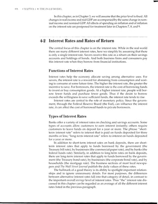
In the top frame of Figurc 4-7, point A shows that the 20 percent rate of
return on the ftrst 757 exceeds the 10 percent interest rate on borrowed funds.
The steplike red line in the top frame of Figure 4-1 shows the rate of return on
the first through fifth planes. The gray area between point A and the 10 percent
interest rate represents the annual profit rate made on the first plane. Point B for
the second plane also indicates a profit. Point C shows that purchase of a third
extra 757 earns only a 10 percent rate of return, or $5 million (10 percent of $50
million) in extra earnings after payment of all noninterest expenses.
Why do the second and third planes earn less than the first? The first plane
is operated on the most profitable routes; the second and third must fly on
routes that are less likely to yield full passenger loads. A fourth plane (at point
D) would have an even lower rate of return, insufficient to pay the interest cost
of borrowed funds. How many planes will be purchased? The third can pay its
interest expense and will be purchased, but the fourth will not. If the interest
cost of borrowed funds were to rise above 10 percent but remain below 15 per-
cent, American would purchase two planes instead of three. If the interest rate
were to fall to 5 percent or below, then American would purchase four planes.
The Interest Rate and the Rate-of-Return Line
The interest rate not only influences the level of business investment but also
affects the level of household consumption. For instance, households deciding
whether to purchase a dishwasher or a second automobile will consider the size
of the monthly payment, which depends on the interest rate. In the bottom
frame of Figure 4-, the rate-of-return line shows that the return on planned
investment and autonomous consumption spending (lr, + Co) declines as the
level of spending increases. As for American Airlines, each successive invest-
ment good purchased by business firms is less profitable than the last. Similarly,
each successive consumption good purchasedby households provides fewer

31. 1)i) ('l l l ''l'1._li I '
'fI IE /.s L 11 ]l( )l)Ei.
!'IGURI,i 4-l
The Pavoff to Investment for an Airline
and the Economy
The red steplike line in the top frame shows
the rate of return to American Airlines for
purchases of additionalTSTs.If the interest
rate is 10 percent, a profit is made by
purchasing the first two pianes, and the
company breaks even by buying the third
plane. Purchase of a fourth or fifth plane
would be a mistake, because the pianes would
not generate enough additional profit to pay
for the cost of borrowing the money to buy
them. The bottom frame shows the same
phenomenon for the economy as a whole.
AN ]NCREASE IN PLANNED PRIVATE SPENDING REDUCES THE RATE
OF RETURN
12345
Numlter of erlra 757s
ttttl
50 1 00 1 50 200 250 300
Cost ($ millions)
500 1,000 1,500 2,000 2,500 3,000
Real private autonomous planned spending (f * C,l
15
10
C
o-
-c=
Otr
cZ .=
20
15
10
c
o_
-c'.=
q)tr
cZ .=
Profit on first
and second planes
r'--t&*r
Loss made on fourth
and fifth planes
Interest rate
----
Loss area
services than the last (for instance, a family's second car is less important and
useful than its first car).
Determination of the level of It) + Cors a two-step process. First we plot the
rate-of-return line representing firms' and consumers' expectations of the bene-
fit of additional purchases. Second, we find the level of In + Co at the point
where the rate-of-return line crosses the interest rate level.
When the interest rate is 10 percent, as in Figure 4-1, autonomous planned
spending (1, + Cr) will be $1,500 billion at point C, as long as the level of busi-
ness and consumer optimism remains constant. A decrease in the interest rate
will increase purchases (10 + Co);for instance, a decrease from 10 percent to 5
percent moves autonomous planned spending from $1,500 billion at C to $2,000
billion at D.
Business and Consumer Optimism
Can purchases ever change when the interest rate is held constant at 10 percent?
Certainly-an increase in business and consumer optimism about the expected
payoff of additional purchases can shift the entire rate-of-return line to the right,

32. TI{E RELATION OF' rLI'fON0lOLfS PL;N}iFlD SI)l.lNDlN(; TO l'lIE IN'l'|,tilt>'t li,'l'11 91
FIGURE 4.2
Effect on Autonomous Planned
Spending of an Increase in Business
and Consumer Confidence
The dashed red "original rate-of-return line"
is an exact copy of the solid red "rate-of-
return line" in Figure 4-1.If the level of
business and consumer confidence were to
increase, the spending schedule would shift
rightward to the solid red "ne / rate-of-
return line." If the interest rate were to stay
constant at 10 percent, then autonomous
planned spending (Ao)would increase from
$1,500 billion at point C to $2,000 billion at
point F.
HIGHER BUSINESS AND CONSUMER CONFIDENCE RAISES
AUTONOMOUS SPENDING
P
c
J
b 15
o_
-c
L tl
)Y.
v :w
o3 5
u. .*
500 -|,000 1,500 I (XX) 2,500 3,000
Real private autonomous planned spending (t, + C,,)
F Interest rate
as indicated by the red "neM rate-of-return line" in Figure 4-2. This shifts to the
right (to point F ) the intersection of the rate-of-return line with the fixed hori-
zontal interest rate line.
The events of September 7,2007, caused a sharp decline in business and
consumer confidence, shifting the rate of return line to the left. Among the ini-
tial effects were massive cancellations by airlines of their previous orders for
new aircraft.
Summarizing, we can show the amount of lt, + Cn spending that would
occur at different interest rates and different levels of confidence.
Demand for Io * Co
Interest rate
15
It)
5
Original ritte-of'-
return line
(pessinristic
c'xpcctations )
1,000 (at B)
1,5(X) (,rt C )
2,000 (at D)
Neu' higherr rltte-oI-
rctunr lirrc'
(optirnistic
t'x1)t'r'tlrtirrti> i
1,500
2,(XX) (at / )
2,500
The left-hand column (pessimistic expectations) is plotted as the "original
rate-of-return line" (red dashes) in Figure 4-2.The right-hand column (optimistic
expectations) is plotted as the solid red "new rate-of-return line."
The Demand for Autonomous Planned Spending
You learned earlier that there are five components of autonomous planned
spending (Ar): planned investment, autonomous consumption, government
spending, the effect of autonomous taxes on consumption, and net exports. We
have already seen that planned investment and autonomous consumption both
depend on the interest rate; both types of spending are stimulated by a lower
interest rate.

33. 92 CilAPTFtR 4 .
FIGURE 4.3
Relation of the Various
Components of Autonomous
Planned Spending to the
Interest Rate
The rrertical black line shows that three
components of autonornous planned
spending do not clepend on the interest
rate. These are governmcnt sperrding
(C), the effect of autonomclus taxes
(-cT), and net exports (NX). The slopred
line shor,r,s that autonomous consumption
(C,,) and planne.d investment (1,,,) depcnd
inversely on thc interest rate. Hence, the
total dernand fclr arutonomous plannecl
spending, as showrr by the "A' clemand
schedlrle," also clepends inversely on
the interest rate.
BOTH CONSUMPTION AND INVESTMENT BY BUSINESS F'IRMS
RESPOND TO THE.INTEREST RATE,
Autonomous p lanrrecl sperrcli rrg (A,,)
c)
AJ
C
1,'
r
,- clt'nr.rncl
sc ht'rlLrlt'
In Figure 4-3 we plot the relationship of the compollents of autonomous
planned spending on the horizontal axis to the interest rate on the vertical axis,
The negative relationship between the interest rate and both planned invest-
rnerrt and autonomolls consumption (/,, + C{,) is copied from Figure 4-2. The
other three components of atrtonomous spending do not depend on the interest
rate.l Accordingly, the total amount of government spending, the effect of
autonomous taxes on consumption, ancl net exports G - cTo + NX) are plotted
as a black vertical line in Figure 4-3.
Total autonomous planned spending also consists of autonornous con-
sumption (C,,) ancl planned investment (1,,), both of which depend negatively on
the interest rate, so thc sl1lout1t of tlrcse trtto s1111rroneris ttdcled to tlrc first flrcc
deptctuls on tlrc intcrest rntc.The lower the interest rate, the larger C,, and the larger
1,,. The total of all five components is shown by the line on the right labeled "4,,
demand schedule." This schedule shows that the total of all autonomous
planned spending depends orr the interest rate.
Shifts in the Ao Demand Schedule
As before, government spencling, taxes, and net exports are given exogenorls
amounts. A chernge in any of these will shift the A,, demand schedule. As you
previously leamed, a shift of business expectations toward optimism and confi-
dence i,t,ill boost planned investment at any given interest rate, so such attitudes
will also shift the A,, demand schedule. Finally, an improvement in consumer
confidence will raise autonomous consumer spending and shift the schedule in
the sarne wav.
lChapter 6 identifics an indirect iink between the interest rate arnr-l net cxports, workirrg throtrgh the
foreign exchange rate. Tlris link is ignorecl lrere.

34. THE RELATION OF AUTONON,IOUS PI,ANNED SPENDING TO TI{E INTEREST RATE 93
J,Vlonetary poiicy is carried out by the Federal
Reserve System (or the "Fed" for short). Roughly
every five weeks, an important meeting is held by the
Federal Open Market Committee (FOMC), which con-
sists of the seven governors of the Fed plus the presi-
dents of the twelve regional Fed banks (e.9., the
Federal Reserve Banks of New York, Chicago, and
Atlanta). At precisely 2:75 P.M. Eastern time, an
announcement is issued as to whether the FOMC has
decided to raise, reduce, or leave unchanged the fed-
eral funds rate, an interest rate that banks charge each
other for lending or borrowing bank reserves (see
Chapter 13). In 2001 and early 2002, the FOMC
responded to perceived weakness in the economy
with unprecedented speed, cutting the federal funds
rate at eleven straight meetings from 6.5 percent at the
end of 2000 to 1.75 percent in January 2002.In other
periods in the past, the Fed perceived that the econ-
omy was too strong and raised interest rates, most
recently Ln7994 and again in7999-2000.
How do these changes in the federal funds rate
influence spending? In the text, the effect of lower
interest rates is depicted in Figures 4-1 and 4-2 as stim-
ulating an increase in planned investment and
autonomous consumption. Indeed, in 2001-02, thre
rapid decreases in interest rates achieved by the FOMC
stimulated consumer spending, especially on autos
and houses. Because of low interest rates, auto compa-
nies could afford to charge very low interest rates to
their customers, even zero interest rates in the fall of
2001. Auto purchasers who might have waited for
months or years raced to showrooms and bought cars
at a record pace. Similarly, low interest rates allowed
more home buyers to qualify for mortgages, or allowed
them to buy bigger houses. In addition, many other
homeowners were able to refinance their mortgages,
lowering their monthly payments (leaving more
money for other purchases) and/or raising the amount
of the mortgage in order to obtain extra cash without
an increase in the monthly payment.
The effect of lower interest rates on consumption
expenditures is one of four "channels" by which the
Fed influences total spending. And the potent impact
of lower interest rates on consumption spending in
2001-02 suggests that this first channel was operating
with great efficacy. However, there are three other
channels of monetary influence, and none of these was
operating normally.
The second channel is the influence of lower inter-
est rates on planned investment. The 2001 recession
had been caused primarily by a collapse in high-tech
inrrestment, particularly investment in computers,
software, and telecommunications equipment. Lower
interest rates did not stimulate spending on those
products because the economy was awash in excess
high-tech equipment; if a firm owns 100 computers
and is only using 50 of them, lower interest rates will
not induce the firm to buy more computers.
The third channel of monetary influence works
through the stock market. Normally lower interest
rates boost stock prices, thus stimulating both con-
sumption and investment spending. But stock prices
fell in both 2000 and 2001 and by May 2A02were 30 per-
cent below their values of two years earlier.
The fourth and final channel works through the
exchange rate. As we will learn in Chapter 6, lower
interest rates cause the exchange rate of the dollar to
depreciate, making U. S. exports cheaper for foreigners
to buy, thus boosting net exports (a component of
CDP). However, instead of depreciating, the dollar
appreciated (became more expensive) throughout 2001.
The first channel of monetary influence, the effect of
lower interest rates in stimulating consumption, was
clearly a very important reason why the recession of
2001 was so mild. But, nevertheless, the economy
remained weak and unemployment rose despite the
rapid action of the FOMC. Some commentators have
described the Fecl in 2001 as "a four-cylinder engine
running on only one cylinder."

35. 9+ ('ll,l)'l'flli ,1 . l'Hli IS-l.ll IlOt)El-
ffiNi' Explain how the A, demand schedule will shift to the left, right, or not at all
in response to the following events:
1. A reduction in auto imports from |apan as the quality of American-built
cars improves.
2. The stimulus to housing given by lower mortgage interest rates.
3. Higher taxes levied by the government in an attempt to reduce the budget
deficit.
4. Higher government spending on security at airports.
5. A reduction in consumer confidence after the September 11 attacks.
The 15 curve is the
schedule that identifies the
combinations of income
and the interest rate at
which the commodity
market is in equilibrium;
everywhere along the 15
curve the demand for
commodities equals the
supply.
4-4 The /S Curve
You have now learned that total autonomous planned spendrng (Ar) depends
on the interest rate. And in Chapter 3 you learned that the total level bf real GDP
and real income depends on the total level of autonomous planned spending.
Now, if we put these two relationships together, we conclude that total real GDP
and real income must depend on the interest rate. In this section we derive a
graphical schedule that shows the different possible combinations of the interest
rate and real income that are compatible with equilibrium, given the state of busi-
ness and consumer confidence, the marginal propensity to save, and the level of
government spending, taxes, and net exports. This schedule is the fS curve.
How to Derive the /S Curve
The lower left-hand corner of Figure 4-4 shows the first ingredient in the deriva-
tion of the 15 curve. The " Au demand schedule" shows the demand for
autonomous planned spending at different levels of the interest rate and is
copied from the "original rate-of-return line" in Figure 4-2. Notice that at a 10
percent interest rate (point C), At)will be $1,500 billion, just the same as (at point
C) in Figure 4-2.To simplify the discussion, initially we assume that there are no
government spending, tax revenue, or net exports, so total autonomous spend-
ing consists simply of the two components, 11., + Cn, both of which depend neg-
atively on the interest rate.'
Mhat will be the equilibrium level of real income if A,, equals $1,500 billion? We
answer this question, just as in Chapter 3,by plotting the level of A, in the upper
right-hand corner of Figure 4-4 as the horizontal red line (with a height of $1,500 bil-
lion). Wrere the An: 1,500line crosses the upward-sloping induced saving line at
point C, equilibrium real income is $6,000 billion. In the lower right-hand side of
Figure 4-4ts plotted the equilibrium level of real income of $6,000 billion against the
assumed 10 percent level of the interest rate.
The figure also shows other possibilities; for instance, at point B in the lower
right-hand frame the assumed 15 percent interest rate is plotted against the
$4,000 billion level of real income that is compatible with it. Point B in the other
frames shows the determination of autonomous spending and induced saving.
'The equation of the A,, demand schedule in the lower left quadrant of Figure 4-4 is:
2,500 - 100r
Thus, when the interest rate is at 10 percent, the level of autonomous planned spending along the
,4,, demand schedule is 2,500 - (100 x 10) : 1,539.

36. WHY EQUILIBRIUM REAL INCOME DEPENDS ON THE INTEREST RATE
4,000 4,000c
;c
o_
z
c
c(g
_C
f>
c;,
<.=
n
c)
c
c
e
f
o
u.=
--
i*
2,000
1,000
0
/t | |
ali,soo
'
1,000 2,000 4,000
Autonomous
planned
spendi ng
2,O00
1,500
1,000
0
20
c
O-
o 10P
;
c
c
o_
qJ l(J
C
In this area, real
income is too high
In this area, real
income is too low
1,000 2,000 4,000 0
Autonomous planned
spending (Au)
FIGURE 4-4 Relation of the IS Curve to the Demand for Autonomous Spending
and the Amount of Induced Saving
In the lower left frame, the "A, demand schedule" is copied from the dashed red line in
Figure 4-2.t shows that the demand for autonomous planned spending depends on
the interest rate. For instance, at a 10 percent interest rate the level of A, is $1,500 billion
at point C. Following the thin dashed black line up from point C and over to the upper
right frame, we see that the economy is in equilibrium at point C, where both A, and
induced savings are equal. This equilibrium level of income is $6,000 billion and is
plotted directly below in the lower right-hand frame at point C, opposite the 10 percent
interest rate that we assumed at the beginning.
1. What interest rate is compatible with an $8,000 billion level of equilibrium
real income?
At what point does this equilibrium occur in
of Figure 4-4?
At what point does this equilibrium occur in
of Figure 4-4?
the lower right-hand frame
the upper right-hand frame
!)ir
Induced saving
10,000 12,ooo
Real income (Y)
/S curve
10,000 12,000
Real income (Y)

37. 9(i ('H,Pl'llR -1 . 'IIJE IS LXI XIODEL
,^{
D r.,." the /S curve is so important and useful, we
pause here to study it more closely. (A full algebraic
treatment of the IS-LM model is given in the appendix
to Chapter 5.)
increase in transfers). Opposite changes will shift
the IS curve to the left.
Figure 4-5 illustrates the effect of a rightward shift in
the Ao demand schedule. The result is a rightward
shift in the 15 curve by an amount equal to the A,
shift times the multiplier.
The multiplier (k) transforms the A,, demand schedule
into the 15 curve. An increase in the multiplier (due,
for instance, to a smailer marginal propensity to
save) rotates or twists the 15 curve outward around
its intercept on the vertical interest rate axis. Thus
the higher the multiplier, the flatter the IS curve.
Anything that makes investment or consumption
demand less sensitive to the interest rate (for
instance, a tendency for firms to pay for investment
goods with internal funds rather than borrowed
funds) rotates or twists the IS curve upward around
its intercept on the horizontal income axis. Thus the
less sensitive the response of autonomous spending
to the interest rate, the steeper the 1S curve.
Diagram Ingredients and
Reasons for Slope
The vertical axis is the interest rate and the horizontal
axis is the level of income.
The 15 curve takes information from two other graphs,
the A, demand schedule and the equilibrium
betwei:n induced saving and autonomous planned
spending. Because A, depends on the interest rate,
and because equilibrium income is a multiple k) of
A' equilibrium income becomes a negative func-
tion of the interest rate.
The horizontal position (equilibrium income) along the
IS curve is equal to the horizontal position along the
A,, demand schedule times the multiplier k.
The 15 curve slopes down because income is a multipie
of A, and A, depends negatively on the interest
rate. The IS curve becomes flatter, the more respon-
sive is A,to the interest rate, and the larger the mul-
tiplier. The 1S curve becomes steeper, the less
responsive is A, to the interest rate, and the smaller
the multiplier.
What Shifts and Rotates the /S
Curve?
The IS curve is equal to the interest-dependent level of
A,, times the multiplier (k). Anything that shifts the
A,, demand schedule will shift the IS curve in the
sd*e direction. The factors that shift the IS curve to
the right include an increase in business or con-
sumer confidence, an increase in government
spending or net exports, and a decrease in taxes (or
What Is True of Points That Are off
the /S Curve?
The entire area to the left of each IS curve is character-
izedby too low a level of production and income for
the economy to be in equilibrium. There is unde-
sired inventory decumulation (negative unplanned
investment, lr,).
The entire area to the right of each IS curve is charac-
terized by too high a level of production and income
for the economy to be in equilibrium. There is unde-
sired inventory accumulation (positive unplanned
investment, Ir,).
At any point off the /S curve there is pressure for busi-
ness firms to adjust production until the economy
returns to the 15 curve.
Because A, depends on the interest rate, equilibrium income does also. The
15 ctrrve in Figure 4-4plots the values of equilibrium real income when the mar-
ginal propensity to save is 0.25 and the multiplier is 4.0, as in the preceding chap-
ter. Notice that points B, C, and D along the 15 curve are all plotted at a horizontal
distance exactly 4.0 times the value of the A, line in the lower left-hand frame.
What the /S Curve Shows
The 15 curve shows all the different combinations of the interest rate (r) and
income (Y ) atwhich the economy's market for commodities (goods and services)

38. cl7
is in equilibrium, which occurs only when income equals planned expenditures.
At any point off the 15 curve the economy is out of equilibrium.
It will be convenient to have a label for the horizontal position of the A,,line,
since this in turn will affect the horizontal position of the 1S curve.'' Let us deJine
A',, as the unlue of autonomous plnnned spendiug thnt would take plnce at 0n interest
rnte of zero.In Figure 4-4 the A, line intersects the horizontal axis at $2,500 bil-
iion, so our label for this A,, line will be A'rn : 2,500. The IS curve always lies at
a horizontal distance 4.0'times the A,, line, because the multiplier (k) rs 4.0.
Notice in Figure 4-4that the 15 curve intersects the horizontal axis at $10,000 bil-
lion, exactly 4.0 times the level of A'po: 2,500.
What Shifts the IS Curve?
Figure 4-4 demonstrates that the horizontal intercept of the 15 curve is always
equal to the multiplier (k) times A',,0, tL.e amount of autonomous planned
spending that would occur at a zero interest rate. Anything that changes Ai,n to
another value like Ai,r will shift the 1S curve. Anything that changes the multi-
plier (k) will rotate the 15 clrrve.
Both the A, demand schedule and the 15 curve will shift to the right if busi-
nesses and consumers become more optimistic and desire to spend more at any
given interest rate.
In Figure 4-5, the ieft-hand frame shows two A,lines. Along the left-hand
"old An demand schedule" confidence is relatively low, but the "new A,
deman& schedule" reflects a higher level of confidence and lies everywherb
exactly $500 billion farther to the right. Since the mtrltiplier is 4.0, the "new 15
curve" lies $2,000 billion to the right, so that at an interest rate of 10 percent,
equilibrium real income is $8,000 billion at point F.
Once again, it is convenient to label each IS curve by the amount of
autonomous planned spending that would occur at an interest rate of zero-
that is, A'p, : 2,500 along the "old ,,4.,, demand schedule" and A'u, : 3,000 along
the "new A,, demand schedule."
The Missing Relation
The 15 curve is like a menu, providing us with innumerable combinations of
interest rates and income that are consistent with equilibrium in the commodity
market. But which item on the menu should we choose? There is not enough
information here to make a choice. We need to find another relationship to link
income and the interest rate in order to tie down the economy's position along
the 15 curve. In the familiar langr-rage of elementary algebra, we have two
unknowns but only one equation. In the next sections, we supply the missing
equation and arrive at a complete theory of how income and the interest rate are
determined."
3We call the IS schedule a " cLrrve," even though we have drawn it as a straight line-, becanse in the
real world the relationship might be a cun'e. Also the' term "IS cttrve" h.ls t'reen iamiliair to genera-
tions of economists since its invention by the late Sir John Hicks iu a classic article, "Mr. Keynes and
the Classics: A Suggested Interpretation," Ecortornctricn, r.ol. 5 (April 7937), pp. 747 -159 .
aDespite its nerme, the 15 cllrve has no unique connection with investment (1) clr saving /S). It shifts
whenever there is a shift in the A,, demand schedule, which can tre causecl by a change in govern-
ment spending, in taxes or transfdrs, or in net exports, as well as by changes in business and con-
sumer confidence.

39. 98 CHAPTI]R ,1 . 'l'l{E IS-L,l,I lOD]ll,
HOW INCREASED CONFIDENCE SHIF'TS THE /S CURVE
2020
c
U
al
g
I rorE
q.)
C
c
6)
(J
o-
9 in
.tr
c
_+
--C I
t
t
l'
I
I
I
1
( )lri /.S,,
1 .-
l
It
0 2,000 4,000 0
Autonomous planned
spending (Ar)
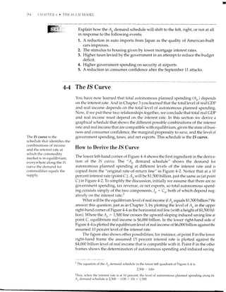
FIGURE 4-5 Effect on the .[S Curve of a Rightward Shift in the
Demand for Autonomous Planned Spending
The "old" A,, demand schedule and IS curve are copied from Figure 4-4. Now we
assume that an increase in the level of business and consumer confidence shifts the Ai,
line $500 billion to the right, just as occurred in Figure 4-2. The 15 curve shifts to tl're
right by four times as much. Notice that the horizontal intercept of the new IS curve at
12,000 is four times the horizontal intercept of the A',,line-that is, A'yt : 3,000.
4-5 Why People Use Money
The second relationship between real income and the interest rate (in addition
to the IS curve) occLrrs in the "money market," a general expression for the
financial sector of the economy. In reality, the financial sector consists of many
assets in addition to money, including short-term debt of corporations and the
government, as well as bonds, stocks, and mutual funds of various types. In this
chapter we n'ill limit our attention to the segment of the financial sector gener-
ally referred to as "money."
The money supply (M') consists of two parts: currency and checking
accounts at banks and thrift institutions. At this stage in the book, the money
supply may be considered to be a policy instrument that the Federal Reserve
Board (the Fed) can set exactly at any desired value, just as we have been assum-
ing that the government can precisely set the level of its fiscal policy instru-
ments-that is, its purchases of goods and services and tax revenues. Later, in
Chapter 13, we will learn how the Fed achieves its control over the money sLrp-
ply in actual practice.
The theory developed in this chapter establishes a link between the rnoney
supply, income, and interest rates. In order to understand the hypothesis
6,000 8,000 10,000 12,000
Real income (Y)
The money supply
consists of currency and
transactions accounts,
including checking
accounts at banks and
thrift institutions.
[u'gf*',+; +rftr rS]
a - l curve to the right

40. c)cl
A medium of exchange is
usecl for br-rying and seli-
ing goods and services and
is a universal alternative to
the barter system.
A store of value is a
method of storing pur-
chasing power when
receipts and expenditures
are not perfectlv synchro-
rrized.
A unit of account is a
way of recording receipts,
expenditures, assets, and
liabilities.
underlying the demand for money, we begin by examining the three traditional
functions of money-its roles as a medium of exchange, a store of value, and a
unit of account.
A Medium of Exchange
The most important function that differentiates money from other assets is its
role as a medium of exchange. Money is one of the most important inventions
in human history because it has allowed society to rise above the cumbersome
method of exchange known as the barter system. With barter, one good or ser-
vice is exchanged directly for another.If , as a professor, I want a leaky faucet
fixed, I must find a plumber who wants to learn about economics. It might take
weeks or months to find such a plumber, since the matching of services requires
a "double coincidence of wants."
A barter society remains primitive because people have to spend so much
time arranging exchanges that they have little time remaining to produce effi-
cientiy. As a result, to avoid arranging exchanges they mustbecome self-strfficient
(I would have to fix my own leaking faucet), thus failing to take advantage of the
essential role of specialization in the development of an advanced economic sys-
tem. Money eliminates the need for barter and the double coincidence of wants.
Which types of assets serve as a medium of exchange? Thirty years ago
almost all exchanges in the United States involved coins, currency, or checking
accounts that paid no interest. Cradually other methods of exchange have
developed, including interest-bearing checking accounts, savings accounts, and
money market mutual funds against which checks can be written. The recluire-
ments for an asset to qualify as a medium of exchange include ready accept-
ability, protection from counterfeiting, and divisibility (ability to use for small
transactions).
A Store of Value
People do not always spend the entirety of their income the instant they receive
it. Some receipts may be spent a day or two iater, but others may be saved for a
substantial period of time. People need some way of storing the purchasing
power of their receipts until a later time. Any asset that performs this function
is called a store of value. There are many financial instruments that serve as a
store of value but not as a medium of exchange, including passbook savings
accounts that do not provide check-writing services, as well as bonds and
stocks. Money can be used both as a medium of exchange and as a store of value.
A Unit cf Account
Money is also used for accounting purposes. How much your employer will pay
you in wages, how much you owe the bank, how much a firm has earned, and
how much a bond is worth are all recorded in some unit of account. This unit is
called dollars in the United States, pounds sterling in the United Kingdom, yen in
Japan, and so on. The dollars entered on accounting records do not physically
exist, in the sense that no coin or piece of currency corresponding to each one
exists in a particular location. Some dollars that serve as bookkeeping entries can
also serve as a medium of exchange without any piece of paper actually changing
hands, as in wire transfers between bank accounts.

41. I0()
Real money balances
eqr-ral the total money
supply divided by the
price level.
4-G Income, the Interest Rate, and
the Demand for Money
The hypothesis that links the money supply, income, and the interest rate states
that tlrc anrourtt of ntoney tlnt peopla tlemnntl in renl terms tleytends botlr on ilrconrc
and on the interest rate. Why do households give up interest earnings to hold
money balances that pay no interest? The main reason is that at least sottc hold-
ing of money is necessary to facilitate transactions, due to the role of money as
a medium of exchange.
Income and the Demand for Money
Funds held in the form of stocks or bonds pay interest but cannot be used for
transactions. People have to carry currency in their pockets or have money in
their bank accounts to back up a check bdfore they can buy anything. (Even ii
they use credit cards, they need money in their bank accounts to keep up with
their credit card bills.) Because rich people make more purchases, they generally
need a larger arnount of currency and larger bank deposits. Thus the demand
for real money balances increases when everyone becomes richer-that is,
when the total of real income. increases.
Changes in real income alter the demand for money in real terms-that is,
adjusted for changes in the price level. Let us assume that the demand for real
money balances M/P) equals half of real income (Y ):
0.5v
The superscript d means "the demand for."
If real income (Y) is $8,000 billion, the demand for real money balances
(M/P)'t wiil be $4,000 billion, as shown in Figure a-6 by the vertical line (L')
drawn at $4,000 billion. The line is vertical because we are assuming initially that
the demand for real balan ces (M/P)'1 does not depend on the interest rate (r).
The Interest Rate and the Demand for Money
The L' line is unreaiistic, however, because individuals will not hold as much
money at a 10 percent interest rate as at a zero interest rate. Why? Because the
interest rate plotted on the vertical axis is paid on asscfs otlrcr thnn ntoney, such as
bonds and savings certificates. The higher the reward (r) for holding interest-
earning financial assets (that are not money), the less money will be held.
If the interest rate (r) paid on nonmoney assets were less than the interest
paid on money, there would be no point in holding them. Individuals wotrld
hold all of their financial assets in the form of money to take advantage of its
convenience. But if the interest rate on them were higher than the interest paid
on money, individuals would cut down on their averafle money holding irr
order to earn the higher interest availabie on aiternative assets. They would con-
sider these higher interest earnings sufficient compensation for the nuisance of
periodically converting these assets into money.
In Figure 4-5 the downward slope of the Lo line through points F and D indi-
cates that when real income is $8,000 billion and the interest rate is zero, the
(ryr' _tl
P/

42. THE I;iI CURVE 101
F'I(;URI'.1.6
The Demand for Money, the Interest Rate,
and Real Income
The vertical line L'is drawn on the unrealistic
assumption that the demand for real balances is equal tcr
half of real income ($8,000 billion in this case), but does
not depend on the interest rate. The L,, curve maintains
income at $8,000, but it allows the demand for real
balances to decrease by $1,000 billion for each 5 percent
increase in the interest rate. The gray area shor,t,s the
amount shifted into other assets, an amount that grows
as the interest rate rises, leaving a smaller and smaller
amount to be held as money.
HOW INCOME AND THE INTEREST RATE DETERMINE
THE DEMAND FOR RE,AL BALANCES
4,000
Real nroney b;rlances WIP)
20
C
_o_
e lfl
rtr
p
c)
c)
C
6,000
Amount shifted into
n0nmtlney assets
1,, {Y - 8,000)
demand for real balances is $4,000 billion. But when the interest rate rises from
zero to 5 percent, people suffer inconvenience to cut down their money holdings
from $4,000 billion to $3,000 billion (point D). When tl-re interest rate is 10 per-
cent, only $2,000 billion of money is demanded (point F ). The new !o line can
be summarized as showing that the real demand for money (M/P)" is half of
income minus S200 billion times the interest rate:
0.5Y - 200r
A change in the interest rate moves the economy up and down its real
money demand schedule, whereas a change in real output (Y) shifts that sched-
ule to the left or right, as shown in Figure 4-7.
(MY
tt:
P /
L.
2.
J.
ffi What are the two determinants of the real demand for money?
What is the effect of each determinant on the real demand for money?
Does a change in either determinant shift the /S curve?
4-7 The LM Curve
Thus far we have learned that the supply of money (M') is controlled by the Fed,
and that the real quantity of money demanded by households (M/P)'/ depends
on both income and the interest rate. Now we can tie these two relationships
together by assuming that the money market is always in e quilibriunt (a situation

43. 102 ('il,Pt'F)i I .
F'IGURE 4.7
Effect on the Money Demand Schedule of a
Decline in Real Income from $8,000 to
$6,000 Billion
The L,, line is copiecl from Figure 4-6 and shor,r,s the
demand for real balances at different rates of interest,
assuming that real income is $8,000 billion. A $2,000
billion drop in the level of incorne to $6,000 billiorr
calrses the dernancl for real bzrlances to drop by half as
much, or $1,000 billion, at each interest rate level. For
insttrnce, at an interest rarte of 10 percent the dem;tnd for
real balances falls from $2,000 billion at point F to $1,000
billion at point C.
A DROP IN THE LEVEL OF'INCOME SHIF-IS
THE MONEY DEMAND SCHEDULE TO THE LEFI
| .-)
1,000 2,000 4,000
Real money balances (MlP)
20
E
(/
!,
a)
g
o 1O
.3
CJ
C
6,000
(Y = tl.O00)
where there is no pressure for change), with the real supply of money equal to
the real demand for money. This equilibriurn condition for the money rnarket
allows us to derive a relationship called the LM umte, just as we prer.iously
derived an equilibrium condition for the commodity market called the 15 currtc,
To achieve equilibrium in the rnoney market,,the real supply of money (Mt/P)
must equal the demarrd for real money (M/P)":
0.5Y - 200r
M' IMN
-tt-
P -p/ - (4 1)
If the amount of money supplied by the government is $2,000 billion and the
price index (P) is set at a constant value of 1.0, then M' /P equals $2,000 billion.
To simplify the analysis, we assume that the supply of money does not clepend
on the interest rate, so Mt / P is drawn in the left frame of Figure 4- B as a verti-
cal line at a level of $2,000 billior-r for every interest rate. The two money demand
schedules, L,, and L1, ate- copied from Figure 4-7.
How to Derive the LM Curve
The sloped money clemand line Ls, drawn
crosses the Mt/P line at point F, where
The demand for money at F is $2,000 billion,
$2,000 biilion. Because the two are equal, the
for an income of $8,000 billion,
the interest rate is 10 percent.
and the supply of money is also
money market is in equilibrium

44. 10ll
A FIXED MONEY SUPPLY IS CONSISTENT WITH MANY DIFFERENT LEVELS OF'INCOME
0 2,000 4,000
Real money balances (MlP)
F'IGURE 4-8 Derivation of t}ne LM Curve
In the left frame the Ln and L., schedules are copied from the previous figure. The
vertical M' / P line shows the available supply of money provided by the government.
The money market is in equilibrium where the supply line (M'/P) ..om"s the demand
line (Lo or L1). When income is $8,000 billion, equilibrium occurs at point l, plotted
:.'iJl'#;:[:11TeH$,'ff :r,"Jt-if :fl ll*?i!:'iH:ffJil:'.il]"n"
shows all combinations of Y and r consistent with equilibrium in the money market.
20
C
I ls
_o_
P
3 io
c
0 2,000 4,000 6,000 8,000 .l
0,000 12,000
Real income (Y)
I (V-Ll ' -
6,000)
when Y : 8,000 (assumed in drawing the Lo line) and r : 10 percent. This
equilibrium combination of values is plotted at point F in the right frame of
Figure 4-8.'
If income is $6,000 billion instead of $8,000 billion, the demand for money is
shown by schedule L, passing through points C and G in the left frame of Figure
4-8. Now the demand for real money balances can be equal to the
fixed real supply of money only at point G, where the interest rate is 5 percent.
Thus Y : 6,000 and r : 5 is another combination consistent with equilibriu.t-t il
the money market, and this is plotted at point G in the right frame of Figure 4-B.n
sThrs, in equation (4.1)
6Thus, in equation (4.1)
2,000 - 0.5(8,000) 200(10)
- 4,000 2,000
- 2,000
2,000 : 0.5(6,000) - 200(5)
: 3,000 - 1,000
: 2,000

45. 104 CI{APTEIT 4 . THII IS-LA,I N,l0DEL
rrr
I he LM curve is as important and useful as the IS
cLlrve. This box explains the slope of the curve and
what makes it shift and rotate its position.
Diagram Ingredients and
Reasons for Slope
The verticai axis is the interest rate and the horizontal
axis is the level of income (same as the 15 curve).
The LM curve shows the different combinations of the
interest rate and income consistent with setting the
demand for money equal to afixed supply of money.
Since the demand for money is fixed everywhere
along the LM curve, but income increases as we
move to the right, "something" must happen to off-
set the higher demand for money that results from
higher income. That "something" is the higher
interest rate, which induces people to shift some
assets into nonmonetary assets, freeing up more of
the fixed available money to be used for the higher
level of transactions.
Along any given LM curve, the level of real money bal-
ances (Mt/P) is fixecl, but real income (Y) varies. The
ratio of real income to real balances is called the
aelocity of money (7);
velocity (Iz) =
#": #
The right-hand expression states that velocity is also
equal to nominal income QY) divrded by the nomi-
nal money supply (Mt).Tlne higher the interest rate,
the higher is velocity. Why? If r increases, people
wish to hold less money. But the money supply is
fixed. To maintain equilibrium in the money market,
there must be an increase in income to induce house-
hoids to hold the fixed existing quantity of money.
Anything that can cause the economy to move up
and down along a fixed LM curve achieves a change
of velocity by altering Y while M' / P is fixed.
What Shifts and Rotates the
LM Curve?
The LM curve is drawn for a fixed real supply of money i
(M'/P). Ahigher nominal supply of money (M') will i
shift the LM curve to the right, as in Figure 4-9, and i
a lower nominal supply of money will shift the LM i
curve to the left. An increase in the price level (P) :
will shift the LM curve to the left, and vice versa i
Anything that makes the demand for money less sen- l
sitive to the interest rate makes both the money ,
demand schedule, L(Y), and the LM curve steeper "
(rotating it upward around its horizontal intercept). ',
Anything that makes the demand for money less i
responsive to changes in income will make the LM i
curve flatter and also shift it outward. .
What Is True of Points That Are off
the LM Curve?
The entire area to the left of the LM curve has an excess
supply of money because income is lower than that
needed to create a sufficient demand for money to
match the supply.
The entire area to the right of the LM curve has an
excess demand for money because income is higher
than required to match the demand for money to
the fixed supply.
At any point off the LM curve there is pressure for
interest rates to change. For instance, when there is
an excess demand for money, people try to obtain
money by selling bonds and other financial assets,
and this pushes up the interest rates on bonds and
other financial assets.
The LM curve is the
schedule that identifies the
combinations of income
and the interest rate at
which the money market
is in equilibrium; on the
LM curve the demand for
money equals the supply
of monev.
What the LM Curve Shows
The line connecting points G and F in the right-hand frame of Figure 4-B is called
the LM curye. The LM curve represents all combinations of income (Y) and
interest rate (r) where the money market is in eguilibrium-that is, where the
real supply of money equals the real demand for money.
At any point off the LM curve, say point D, the money market is not in
equilibrium. The problem at D and all other points in the red shaded area is
that the demand for real money exceeds the available supply.At point C and all

46. TTIE I,T4 CLTRVE 105
other points in the white area there is an excess supply of money that exceeds
the demand.
How does the economy adjust to guarantee that the given supply of money
created by the government is exactly equal to the demand when the money mar-
ket is out of equilibrium, as at point D? One possible adjustment, a reduction in
the price level, will be considered later. In this chapter we continue to assume
that the price index (P) is fixed at 1.0. Without changing prices, the economy
might achieve money market equilibrium from point Dby increasing the inter-
est rate from 5 to 10 percent. This would move it to point l, cutting the demand
for money. Or,instead, income might fall from $8,000 billion to $6,000 billion
while the interest rate remains fixed. This would cause a movement to point G
and would also cut the demand for money. Or some other combination might
occllL with a partial drop in income and a partial increase in the interest rate.
1. By how much does the demand for money change when the economy
moves from point D to point F in Figure 4-B?
2. From point D to point C?
3. From point C to point F?
4. From point C to point C?
What Makes the LM Curve Shift?
The position of the LM curve is determined by the size of the money supply, and
any change in the money supply will cause the LM curve to shift its position.
What happens when the Fed decides to alter Ms, the nominal money supply? If
the price level (P) is fixed, this will alter the real money supply (Ms/P).In Figure
4-9, for instance, a $1,000 billion increase in the money supply from 92,000 to
$3,000 billion shifts the LM curve from the left-hand dashed line (LMi to the
right-hand solid hne (LM). Since each dollar of extra available money makes pos-
sible 2.0 extra dollars of income , the LM curve shifts horizontallv bv $2,000 billion.
Another way to interpret the effect of a higher money supply is also shown
in Figure 4-9. How does the economy adjust if real income remains fixed at
Y : 8,000? In the left frame of Figure 4-9, the demand-for-money line, labeled
Lr(y : 8,000), shows the amount by which the demand for money increases as
the interest rate declines, holding the level of income fixed at Y : 8,000. If the
money supply is at its original value of 2,000, the money market is in equilibrium
at point I, with an interest rate of 10 percent. When the money supply increases
from 2,000 to 3,000, the left frame shows that the interest rate must decline from
10 percent at point F to 5 percent at point D in order to maintain equilibrium in
the money marketbyboosting the demand for moneyby the same amount as the
money supply has risen-that is, from 2,000 to 3,000.
In the right frame of Figure 4-9, points F and D are plotted at the same
horizontal position, since the level of income is assumed to be 8,000. When
the money supply is at the original level of 2,000, the economy operates along
the original LMo curve at point F. When the money supply increases to the new
value of 3,000, the LM curve shifts rightward to its new position LM, at point D.
Which outcome will occur following an increase in the money supply? Will
income increase while the interest rate remains constant? Or will the interest
rate decline (as from point F to point D) while income remains constant? Once
again, we cnnnot determine the unlue of two tmknowns with only one relntion-thnt is,

47. -
106 ('l[APTI']R -l ' TIIFI IS'L]'I N'I()DEI.
HOW A HIGHER REAL MONEY SUPPLY CAN REDUCE THE INTEREST RATE
Higher money
supply shifts
LM curve to right
0 2,000 4,000
Real money balances WIP)
FIGURE 4-g The Effect on the LM Curve of an Increase in the Real Money Supply
from $2,000 Billion to $3,000 Billion
The dashe d LM'line in the figure is identical to LM in Figure 4-8. When the money
supply is increaied, the money available to support output increases and the LM curve
rnifir .ightwa.d by 2.0 dollars per dollar of extra money to the new LM, line.
20
c
9 1s
0.)
1
;O IU
C
0 2,000 4,000 6,000 8,000 10,000 12,000
Real income (Y)
New lM, curve
(+ = 3,ooo)
1,, (Y= 8,000)
the LM curae. We must use both relations, the 1S curve and the LM curve, to
cletermine the two unknown variables-income and the interest rate' The next
section joins together the 15 and LM curves to determine the level of both
unknown variables.
4-8 The /S Curve Meets the LM Curve
Now we are ready to examine the economy's "general equilibrium," which
takes account of behavior in both the commodity and money markets. We do
this by bringing together the ISo curve from Figure 4-5 with the LMo curve from
Figure 4-9.
Equilibrium in the commodity market occurs only at points on the 1S curve'
Figure 4-10 copies the 1S,, schedule from Figure 4-5 drawn for a value of
Aiur: 2,500. Ai any point off tne ISo curve-, for instance G and l, the commod-
ity market is out of equilibrium. C, D, and E,, all represent different combina-
tions of income and the interest rate that are compatible with
commodity-market equilibrium. At which equilibrium point will the economv
come to rest? The single ISo schedule does not provide enough information to
cjetermin e both income and the interest rate. Truo schedules are needed to pin
down the equilibrium values of two unknown variables.

48. NI0NETA1TY I)OI,I('' IN A(]'I-i0 107
FIGURE 4.10
The /S and, LM Schedules Cross
at Last
The 156 schedule is copied from Figure 4-5; the
LMo schedule is copied from Figure 4-9. Only
at the red point, E0, is the economy in "gen-
eral" equilibrium, with the conditions for equi-
librium attained in both the commodity market
(along 15) and the money market (along LM).
At points U, V, G, and E, the commodity mar-
ket is out of equilibrium. At points U, V, C, and
D, the money market is out of equilibrium.
THE ECONOMY'S "CENERAL" EQUTLTBRTUM
20
15
P
c
o_
.g 10
a)
c
4,000 6,000 - ,
( )( !0 8,000 1 0,000
Real income (Y)
2,55A, ft = 4,0)
General equilibrium is a
situation of simultaneous
eouilibrium in all the
mirkets of the economy.
The LM curve provides the necessary additional information, showing
all combinations of income and the interest rate at which the money market is
in equilibrium for a given real money supply-in this case, $2,000 billion. Figure
4-10 copies the LMo schedule from Figure 4-9 drawn for a value of Ms/P : 2,000.
At any point off the LMo curve, for instance points C and D, the money market
is out of equilibrium. At D income is too high and the real demand for money
exceeds the real supply. At C income is too low and the real demand for money
is below the real supply. Equilibrium in the money market occurs only at points
such as G, F, and Es, each representing combinations of income and the interest
rate at which the real demand for money is equal to a real money supply of
$2,000 billion.
How does the economy arrive at its general equilibrium at point E. if it
starts out at the wrong place, such as at points U or V ? If the commodity mar-
ket is out of equilibrium and involuntary inventory decumulation or accumula-
tion occurs, firms will step up or cut production, pushing the economy in the
direction needed to reach E0. If the money market is out of equilibrium, there
will be pressure to adjust interest rates, since people will have to sell stocks and
bonds if they cannot otherwise satisfy their demand for money. Either way the
economy arrives at En.
4-g Monetary Policy in Action
The IS-LM model uses two relations (or schedules) to determine the two
endogenous variables, real income and the interest rate. The exogenous vari-
ables, which the model does not explain, are the level of business and consumer

49. 108 CHAPTER 4 . THE ls-tfll NIODEL
An expansionary
monetary policy is one
that has the effect of
lowering interest rates and
raising GDP.
A contractionary
monetary policy is one
that has the effect of
lowering CDP and raising
interest rates.
optimism, the single instrument of monetary policy (the money supply), the
two instruments of fiscal policy (government sper-rding and tax revenues), and
net exports. Whenever there is a change in one of the exogenous variables, the
result will be a change in either or both of the two endogenous variables, real
income and the interest rate. In this section we will see that a decision by the Fed
to change the money supply will normally lead to a change in both real income
and the interest rate.
What level of real GDP does the Fed desire? We shall assume that the
desired level of income, "natural real GDP," is $8,000 billion. In Figure 4-10 the
equilibrium level of real income (GDP) at point En is only $7,000 billion. Thus
there is a $1,000 billion "gup" between actual and natural real GDP that needs
to be filled. What should the Fed do?
To raise CDP by the required $1,000 billion, the Fed must increase the money
supply. This action is called an expansionary monetary policy. Conversely, if
natural real GDP is lower than actual real CDP, the Fed can decrease the money
supply. This is an example of a contractionary monetary policy.
Normal Effects of an Increase in the Money Supply
Wili an increase in the money supply increase real income, reduce the interest
rate, or both? If the 1S and LM curves have the "normal" shapes displayed in
Figure 4-70, the answer is "both." As we shall see in the next chapter, there are
extreme cases in which the 15 and / or the LM curres are vertical or horizontal,
and the entire impact of a change in the money supply may fall just on real
income or just on the interest rate. But here, where the 15 curve has its normal
negative slope and the LM curve has its normal positive slope, monetary policv
changes both real income and the interest rate.
Figure 4-11 repeats the LMo curve of Figure 4-70, drawn on the assumption
that the real money supply is $2,000 billion. Also repeated is the lSo curve of
Figure 4-10, which assumes that A'po:2,500 and k: 4.0. The economy's gen-
eral equilibrium, the point where both the money and commodity markets are
in equilibrium, occurs at point E,,.
Assume that the Fed now raises the nominal money supply from $2,000 bil-
lion to $3,000 billion. As long as the price level stays fixed at 1.0, the real money
supply increases by the same amount. The LM curve shifts to the right by $2,000
billion. Now, at the new higher real money supply of $3,000 billion, there is an
"excess supply of money" of $1,000 billion. How can the economy generate the
$1,000 billion increase in the real demand for money needed to balance the neu'
higher supply?
Finding themselves with more money than they need, individuals transfer
some money into savings accounts and use some to buy stocks, bonds, and com-
modities. This raises the prices of bonds and stocks and reduces the interest rate.
The lower interest rate raises the desired level of autonomous consumption and
investment spending, requiring an increase in production. Only at point E,,
with an income level of $8,000 billion and interest rate of 5 percent, are both the
money and commodity markets in equilibrium. Compared to the starting point
En, the increase in the real money supply has caused both an increase in real
income and a reduction in the interest rate.
Monetary policy works exactly the same in reverse. If the desired ler.,el oi
real income was not $8,000 billion but rather $7,000 billion, the Fed could
move the economy leftward from point E, in Figure 4-11 to point E6, simplv

50. HOV F'ISI]AL EXPANSION CAN "CROWD OUT'' I}.iVEST1I}'NT 109
FIGURE 4.11
The Effect of a $1,000 Billion
in the Money Supply with a
Normal LM Curve
fncrease 2o
We repeat the $1,000 billion increase in the
money supply that was shown in Figure 4-9.
In order to maintain equilibrium in both the
comrnodity and money markets here, two
effects occLrr: equilibrium income rises and the
interest rate declines, as indicated by the
movement from Eo to Er.
A HIGHER MONEY SUPPLY BOOSTS INCOME AND CUTS THE INTEREST RATE
c
o 10
o
CJ
c
2,OOO 4,000 6,000 7,000 ii,(xx) 10,000 12,000
Real income (Y)
Old lM,,curve /
(ry = 2.ooo) | P '/
New lM, curve
(+:3,ooo)
Equilibriunr
moves to nere
by reducing the real money supply from $3,000 billion
result, the LM, curve would shift leftwards to LMo, and
from $8.000 billion to $7,000 billion.
to $2,000 billion. As a
income would decline
4-10 How Fiscal Expansion Can "Crowd Out"
Investment
In the last section we exarnined the effects on real income and the interest rate
of changes in monetary policy by shifting the LM curve along a fixed 15 curve.
Now we shall do the reverse and shift the 15 curve along a fixed LM cun,e. The
original 15 curve is copied from Figure 4-10 and is labeled in Figure 4-12 (on
page 772) as the "old lSo curve " ; it is drawn on the assumption that the amount
of autonomous planned spending that would occur at a zero interest rate (Ai,o)
is equal to $2,500 billion.
Expansionary Fiscal Policy Shifts the /S Curve
An expansionary fiscal policy taking the form of a $500 billion increase in gov-
ernment purchases shifts the 1S curve to the right. Note that the horizontal dis-
tance between the old and new 15 curves is not $500 billion but $2,000 billion,
since the horizontal shift of 15 is $500 billion times the multiplier, still assumed
to be 4.0.
Figure 4-72 demonstrates that the effect of an expansionary fiscal policy on
real income is not indicated by our original Chapter 3 multiplier (k : 4.0) once

51. 110
II{TERNATIONAL i The Wbrldwide Effects on Consumer
PERSPECTIVE
i
Confidence of the September 11 Attacks
la
I
rn
I he September 77, 2007, attacks were felt most
directly in downtown Manhattan and at the Pentagon.
But the first significant foreign attack on the American
homeland, lr,,hich had been immune in previous wars,
dealt a blou, to the American psyche. Trips were can-
celled and vacation plans postponed, and the airline
and hotel industries went into a tailspin. Sales of lux-
ury goods suffered, as wealthy individuals felt Llrlcorn-
fortable inclulging themseives while others were
suffering.
The arnalysis in Chapter 4 singles out consumer and
business confidence as factors that can shift autonomous
planned spe.nding and the 1S curve. The September 11
attacks stand out as a clarssic case of an adverse "shock"
to consumer ancl business confidence. In terms of our
macroeconomic model, the attacks caused the 1S
curve to shift to the left, thus reducing the level of
planned expenditures at any given interest rate.
Monthlv surveys measure the state of consumer con-
fidence in the United States; the figure displays the
Irrdex of Consumer Confidence for 7988-2002 as com-
piled by the Conference Board.
Clearly, there was a sharp drop in consumer confi-
dence in October and November 2001 as a result of the
attacks. Hor,r,ever, several remarkable facts stand out
from the graph. First, the e.ffect of September 11 was
short-lived, since confiderrce snapped back over the
next few, months. Second, the post-;'rttack drop in con-
sumer confidence was much smaller than the sharn
decline in confidence that began in mid-2000, which in
turn represented a reaction to the beginning of a
decline in the stock market and a turnaround in the job
market from rapid job growth to layoffs and vanishing
jobs. The post-attack drop in consumer confidence was
also much smaller than that which occurred after the
August 1990 invasion of Kuwait by Iraq or in several
other episodes in the early 1990s. Overall, while the
post-attack period provides an example of a drop in
consumer confidence that shifts the IS curve to the left,
it was relatively minor and short-lived compared to
other episodes.
The effects of the September 11 attacks were not
lirnited to the United States. Many other nations lost
citizens who had been working in the World Trade
Center that morning-hundreds in the case of the
United Kingdom and Japan. Yet the impact of the
attacks on consumer confidence in other countries
was even smalier than in the United States, perhaps
because these citizens were farther away from thc.
World Tiade Center and were concerned with differ-
ent issues.
For instance, Japan had been mired in a decade-long
slump (we will learn more about this in Chapter 5).
Consumer and business confidence had been declining
for a long time, and the attacks barely registered a rip-
ple on a sea of pessimism caused by a persistent
decline of industrial production, a continuing loss of
jobs, and the seeming inability of policymakers to take
i
the money market is taken into consideration. The full fiscal multiplier of k : 4.0
would move the economy horizontally from the initial equilibrium position at
En to point E2, where income is $2,000 billion higher. At E2, however, the money
market is not in equilibrium, because E, is off the LMo curve. Income is higher
than at Es, raising the dernand for money, but the real supply of money remains
unchanged at the original assumed value Mt/P :2,000. There is an excess
demand for money.
To cut the demand for money back to the level of the fixed supply, the inter-
est rate must rise. But an increase in the interest rate makes point E, untenable
by reducingplanned consumption and investment expenditlrres. Only nt poinf E.
are both the commodity and money markets in equilibrium. Real income does
not increase by the full $2,000 billion, but only by half as much, $1,000 billion.
The higher interest rate accounts for the fact that the fiscai policy multiplier
is 2.0, rather than 4.0, r,t'hen the requirement for money market equilibrium is

52. FIOV I'I S(]AL EXPANSION (]AN *CRO'D (]T]T" I N V I,] S1' N I E NT 111
the strong actions that many observers agreed were
needed. At the other extreme was France, where con-
sumer confidence hit all-time highs in late 2001 and
early 2002. The French economy was expected to con-
tinue growing at the most rapid rate of all the large
European countries, and French consumers reported a
record-high readiness to purchase cars and houses, as
well as optimism about the outlook for their own
household finances.
The ripple effects of the September 11 attacks
impacted the U.S. economy, and this amplified a sharp
decline in U.S. imports that was already underway and
that reduced net exports in many economies, particu-
larly in Asia. But, aside from the effect on foreign trade,
the attacks had virtually no separate impact on con-
sumer confidence in other countries, while even within
the United States, the slide in consumer confidence
was surprisingly small and short-lived.
.,1'
oL
1 9BB 1 989 1 990 1991 1992 1993 1994 1 995 1996 1997 ',r
998 1999 2000 2001 2002 2003
Source: The Conference Board
taken into account. The increase in the interest rate from 7.5 to 10 percent cuts
private autonomous planned consumption and investment spending by $250
billion, fully half of the $500 billion increase in government spending. Thus fully
half of the original multiplier of 4.0 is "crowded out."
Comparison of Equilibrium Positions Eo and Eg
120
110
100
il90
x --
-o
c
70
Initial8,,
Interest rate (r) 7.5
Private autonomous spending Qp + C,,: 2,500 - 100r) 7,750
Government spending (C) 0
Total autonomous spending (A, : I, I C,? + C) 1,750
Income (Y : 4.04t)) 7,000
Ncu, E,
10.0
1,500
500
2,000
8,000

53. E
II2 tlltAPTb'It .1 . THI| I,S-LXI IIODiil,
THE CROWDING OUT EFFECT CUTS THE, FISCAL MTJLTIPLIER
tur(# = 2,ooo)
0 2,000 4,000 6,000 7,000 8,000 (),i)00 10,000 12,000
Real income (Y)
FIG{JRE 4-12 The Effect on Real Income and the Interest Rate of a $500 Billion
lncrease in Government Spending
Along the original 1S., curve, the autonomous spending desired at a zero interest rate
(A1,,) is 2,500 ancl the economy's equilibrium occurs at point Eo.A $500 billion increase
in governrnent spending boosts spending from A'ro : 2,500 to A'4 : 3,000, ancl shifts
l;ilr#ffi j;#ll#;;:Irfi*iHLfrii#*r"ilsf:;ilt:ffi-
is partial, not complete.
15
a.)
g
d,
(-)
0)
CJ
I
I
-t
l
I
i
i
I
Crowding
out effect
The crowding out effect
describes the effect of an
increase in government
spending or a reduction of
tax rates in reducing tlre
amount of one or more
other components of
private expenditures.
The Crowding Out Effect
Some economists and journalists use the phrase crowding out effect to compare
points such as E, and E, in Figure 4-I2. The $1,000 billion difference in real
income between points Erand E, results from the investment and consumption
spending crowded out by the higher interest rate. Point Er, used in calculating
the size of the crowding out effect, is a purely hypothetical position that the
economy cannot and does not reach. Actually, far from being crowded out, total
private spending is higher in the new eqlrilibrium situation at E. than at the
original situation at Eo-real income has increased by $1,000 billion, of which
only $500 billion represents higher government purchases, leaving the remain-
ing $500 billion for extra private expenditures. The composition of private
spending changes, however, as a result of the higher interest rate. Induced con-
sumption spending increases, but autonomous private spending decreases,
Expenditlrres are divided up as follows in the two situations:

54. SL]NIIIARY
At O.,
500
1,500
6,000
8,000
113
Covernment purchases
Autonomous private spending (lp + Ca)
lndtrced consumption
Total real expenditures
At E0
0
7,750
5 ?50
z;,ntoo
Can Crowding Out Be Avoided?
The fundamental cause of crowding out is an increase in the interest rate that is
required whenever income rises and the supply of money is fixed while the
demand for money responds positively to an increase in income. To offset the
increase in the demand for money caused by higher income, it is necessary for
the interest rate to rise by enough to offset the effects of higher income on the
demand for money.
The simplest way to avoid crowding out would be for the Fed to increase the
money supply, thus allowing the LM curve to shift rightward by the same
amount as the /S curve. Another possible exception to crowding out would be if
the demand for money did not depend on income. Other hypothetical situations
in which crowding out would be avoided are when the 15 curve is vertical (that
is, the interest responsiveness of spending is zero) or when the LM curve is hor-
izontal (that is, the interest responsiveness of the demand for money is infinite).
In the next chapter we will begin by examining some of these situations in
which monetary policy and fiscal policy are unusually strong or weak, then study
interactions among monetary and fiscal policy, and finally learn about effects of
the government budget surplus or deficit on trade, investment, and growth.
1. Interest rates allocate the supply of funds available
from savers to alternative borrowers. Not only do pri-
vate households and firms borrow in order to buy
consumption and investment goods, but the govern-
ment also borrows to finance its budget deficit.
2. Private autonomous plannecl spending W) depends
partly on the interest rate. The higher the interest rate,
the lower is A,,.
3. Private autoiomous planned spending (Ar) also
depends on the optimism or pessimism of investors
and consumers about the future. An increase in optr-
mism tends to raise A, for any given level of the inter-
est rate.
4. The 1S curve indicates all the combinations of the
interest rate and real income at which the economy's
commodity market is in equilibrium. At any point
off the IS curve, the commoditv market is out of
equilibrium.
5. The main functions of money are its use as a medium
of exchange, a store of value, and a trnit of account.
6. The real quantity of money that people demand
depends both on real income and on the interest rate.
Equilibrium in the money market requires that the real
supply of money equal the demand for real money
balances.
7. The LM curve represents all the combinations of real
income and of the interest rate where the money mar-
ket is in equilibrium.
8. An increase in the money supply raises real income
and reduces the interest rate when the 15 curve has its
normal negative slope and the LM curve has its nor-
mal positive slope.
9. A fiscal expansion raises reai income and the interest
rate, causing crowding out if the money supply is held
constant and both the 15 and LM curves have their
normai slopes.

55. i1+
Note: Asterisks designate Concepts, Questions, and Problems that require the Appendix to Chapter 3.
rate of return
15 curve
monev supply
medium of exchange
store oi value
unit of account
real money balances
LM curve
general equilibrium
expansionary monetary policy
contractionary monetary policy
crowding out effect
,i:r r
QUITSTTONS
1. Which among the exogenous variables listed in ques-
tion 1 at the end of Chapter 3 have become endoge-
nous in the cornplete IS-LM model of this chapter? Is
this true as well for autonomous consumption expen-
cliture? Velocity? Have any othe.r endogenous vari-
atrles been introducecl in this chapter? Exogenous
variables?
2. Suppose that in early 2001 many econornic forecasters
preclict that a rnajor recession will occur in late 2001 or
early 2002. How might these forecasts affect the actual
performance of the economy in 2001 and2002?
3. Describe the automatic adjustment that will take place
in the economy when the current position of the econ-
orny is off the 15 curve.
4. Describe the automatic adjustment that will take place
in the economv when the current position of the econ-
omy is off the LM curvc.
5. Why is the distinction between autonomous expendi-
ture and induced expenditure crucial to an under-
st;rnding of the crort'ding out effect?
6. Under r,r,hat circumstances could government spend-
ing (federal, state, and local) be crowded out? Do you
think this is likely to be the case?
7. Whart happens to the velocity of rnoney (defined in the
box on p.10a) when the economy mores along a given
LM cr,rrve? Why does velocity behave this way?
8. Describe the situation in the commodity market ancl
the money rnarket at point V in Figure 4-10. What will
happen to the econolny if the current position is at
point 7?
9. During the 1980s the size of the federal government
debt became so large that servicing the interest pay-
ments became a significant portion of total federal
expenditure. In response, many representatives and
senators felt that the federal deficit needed to be
reduced. If government spending (G) became nega-
tively sensitive to changes in the interest rate, what
effect would this have on the slope of the 15 curve? If
atttonornous taxes (tr) become positively sensitive to
changes in the interest rate, what effect would this
have on the slope of the IS curve?
10. A change in which of the follor,r'ing would cause the IS
curve to shift? To rotate? To both shift and rotate?
Which do not affect the position or slope of the 15
curve?
(a) autonomous planned expenditure at zero interest
(A")
@) mdrginal tax rate (t)
(c) rnarginal propensity to 531rs (s)
(d) share of imports in GDP (irr)
(e) interest rate (r)
(f) multiplier (k)
(g) interest sensitivity of the An demand schedule
(h) business and consumer confidence
11. A change in which of the following would cause the
LM curve to shift? To rotate? To both shift and rotate?
Which do not affect the position or slope of the LM
curve?
(a) nominal rnoney supply (M')
(b) responsiveness of the demand for money to the
interest rate

56. tz.
(c) responsiveness of the demand for money to
income
(d) business and consumer confidence
(e) interest rate (r)
(0 price level (P)
Suppose Congress raises autonomous taxes. How will
this tax hike affect real income? The interest rate?
Consumption? Planned investment?
13. If the A,, demand schedule shifts to the right, r.l'hat
happens to the real interest rate? Does the chan5;e in
real interest rate amplify or dampen the swings in
income that result from changes in,4,,?
14. You learned in Chapter 1 that infltrtion speeds up
when actual real GDP exceeds natural real GDP. If pol-
icymakers believe that actual real CDP is too high and
fear that inflation r.t,ill rise, how could they use lnone-
tary and fiscal policies to reduce actual real GDP?
Describe how each policy woulcl work ancl its effects
on the economy.
15. Evaluate the follou,ing argument trsing the 1S-LM
model: When consumer and business confidellce are
high and the economy is booming, the interest rate is
high. Therefore, cluring a recession the Fed could pro-
mote tr higher ler.el of income if it trsed monetary pol-
icv to raise the interest rate.
PR(}I]LEMS
*1. Let the structure of the commodity rnarket be repre-
sented by the following equations: C : Cu +
0.75(Y T), C,, : 200 70r, T : 200 + 0.2Y,
1,. : 300 - 3]r,ernd C : 400.
thl Wnat is the value of the multiplier (k)7
(b) What is the equation of the autonomous planned
expenditure iurrctir-rn? (Hirtt: Just substitute the
erluations given above for C,,, T, and 1,, .rnd the
value given above for G into the geueral formttla
for A,,: A,,: C,, - cTn + It, + G + NX,/. In this prob-
lem NX,, : 0.)
(Jlrt]sTloi{s rNI) f,R( )BLF}tS I 1 ir
and parameters /r and/in the LM curve: Mt /P = 300,
h:0.1, and/:50.
(a) What is the horizontal intercept of the LM curve?
(b) What is the slope (Lr / LY ) of the LM curve?
(c) What is the equtrtion of tlre LM cun,e?
(d) If the Fed increased the money supply by 100, at
r.vhart value on the horizontal axis r.r,ould the LM
curve intersect it? What happens to the slope of
the LM curve?
*3. Using the inforrntrtion contained in problems 1 and 2,
what is equilibrium real income (Y) and the interest
rate (r)
(a) in the inititil situation (i.e., G : 400, M' / P - 300)?
(b) if C increases to 450? What is the amount of
autonomous spending that is crolt'ded out irr this
situ.-rtion? What happens to velocitv?
(c) if M'/P increases to -100?
(d) if both C antl M'/P increase (i.e., C : 450 ancl
M' /P - 4oo)?
*4. Assume that the economv is initially in equilibriunr at
a ler..el of real output (Y) oi $5,000 ancl an interest rate
(r) ctf 5 perccnt. If as a result of an incrcase in govern-
ment spending of $500, the economy rrloves to a new
eqr-rilibritrm at Y : $5,750 trncl r : 6.5 percent (.rud
given that k : 3), how much Y woulcl be crowded ottt
due to the increasc in the interest rate? How much
autonor-rrous spencling r,t,oulc1 be cror,r,ded out? What
is the value of the cocfficient for intercst-rate r€'spon-
o siveness of the 15 curve? Of the A,, dernand schcdule?
*5. Assume that the following ecl,rations summarize. the
structnre of an ecolromy.
C: C,, + 0.8(Y - T);
C,,: 700 - 15r;
T :200 + 0.2Y;
(M/P|l : 0.7Y - 70r; M'/P: -1.10;
/,, : 500 25r;
i - 1,100;
NX: 100 - 0.04Y.
Answer the follovviug questions:
(a) What is the ecluation of the 15 cun,e?
(b) Whtrt is the eclttation of the LM cun,e?
(c) What is the equilibritrm retrl output?
(d) What is the erprilibrium interest rate?
(e) What is the level of saving at equilibrium?
(f) What is the level of planned investment at eqr.ri-
libriurn?
(g) Determine r.t,hether leakages equ;rl injectiorrs at
equilibrium.
(h) Assr.rme that r : 4 arrcl Y : 5,t100. Is there an
excess denrtrnd for money or cxcess suprply of
money in this situatictrr? Hort, mttch? Is there
unplanned inventory change? If so, what is the
vahre of the urrplannerl irrventory change?
What is the equation of the IS curr.e? (Hirrf: The
general equation for tht. 15 curve is Y : kA,,.)
Wlrat is the slope of the /S curve (r / LY )?
If government spencling increased by 50, zrt what
value on the horizontal axis would the new 1S
cllrve intersect it? What would happen to the
slope of the 15 cun'e?
*2. The equation of the LM ctrrve is given by the follow-
ing formula: Y : l(M'/P) + frl/lt, where M'/P is the
real money sr-rpply, /r is the response of money
derr-rand to a $1 change in income at a fixecl interest
rate, and/ is the response of money demand to a one
percentage point change in the interest rate. Assume
the folkrvving values for the exogenous yariable M'/P
(c)
/.-t
Ll/
(e)

57. 1 16 CHAI'}I'ER .1 . l'HIi IS-LM IIOllitL
p. 94 (1) A reduction of imports raises net exports and
shifts the A,, demand schedule to the right. (2) A change
in interest rates moves the economy nktug the schedule
but does not shift it. (3) Higher taxes reduce consunp-
tion and thus shift the A.. demand schedule to the left.
(4) Higher go.cmment spendirrg shifts the A,, demand
schedule to the right. (5) A recluction in consumer con-
fidence shifts the 4.. demand schedule to the left.
p.95 (l)An irrterest rhte of 5 percent is compatible with a
$4,000 billion level of equilibrium retrl income. (2) This
occurs at point D on the 15 curve in the lower right-hand
frame oi Figure 1-4. (3) This eqr-rilibrir-rm occrlrs at point
D in the upper right-hancl frame of Figure 4-4.
p.101 (1) The levels of it'rcome (Y) and the interest rate on
assets other than money (r) are the tn o determinants of
the real demernd for money, (M/P)'t. (2) An increase in Y
raises the real demand for money, and an increase in the
interest rate reduces the real demand for money.
(3) Ne.ither determinant shifts the 15 cLrrve, because the
axes of the /S crlr/e diagrarn are these very determi-
nants, Y and r.
p.105 (1) ln going from D to E, the irrterest rate rises from
5 to 10 percent, ancl the demand for money decreases bv
the interest responsiveness (200) times the change in the
interest rate (S)-that is, by 1000. (2) In going frorn D to
G, the level of real income falls from 8,000 to 6,000. The
demand for money decreases by the income respon-
siverress (0.5) times the change in real incorne (2,000)-
that is, by 1000. (3) This is the reverse of Part (2); the
demand for money increases by 1000. (-1) This is the
reverse of Part (1). The dernand for money increases by
1000.
I
F
hi