This document summarizes an interactive evolutionary algorithm called DARWIN for robust multi-objective optimization. DARWIN was developed by Greco, Matarazzo, and Slowiński. It combines interactive multi-objective optimization and evolutionary algorithms to find solutions that best fit a decision maker's preferences while also handling uncertainty in the problem formulation. The author implemented DARWIN and conducted computational experiments to evaluate its performance on different test problems and understand the impact of various parameter settings.


![6 1 Introduction
then the solution is called robust. The same applies if the problem model can not be formulated
precisely — for example, it contains a value that may be only estimated, like the future price
of a raw material. The solution should be resistant to small fluctuations in the problem’s model
parameters. The robustness in MOO context is the ability to withstand changes in the parameters
and in the problem formulation; it is a very important quality of any MOO technique.
To give final recommendation instead of the Pareto-frontier one has to engage the decision
maker in the process. The method has to be interactive in order to gather the DM’s preferences.
It can be done by showing exemplary feasible solutions and asking the decision maker to rank
them or simply by asking about the inter-criteria trade-offs. These preferences are used to guide
the search of the solution space in the directions desired by the DM. An optimization technique
involving interaction with the decision maker is called the interactive multi-objective optimization
(IMO) technique.
The algorithm is a well-defined list of instructions for completing a task. Several researchers
suggested that principles of the evolution — particularly, the concept of population and survival of
the fittest individuals can be a good model of operation for multi-criteria optimization algorithms.
Methods using these principles are called the evolutionary algorithms (EAs) while the whole field
of research is the evolutionary multi-objective optimization (EMO).
In this paper, the author presents a software implementation of the DARWIN method and
the first large computational experiment with DARWIN. DARWIN is an acronym for Dominance-
based rough set Approach to handling Robust Winning solutions in INteractive multi-objective op-
timization. It has been proposed by Salvatore Greco, Benedetto Matarazzo and Roman Slowi´nski
in [9, 13, 14, 15] for solving multi-objective optimization problems. It interacts with the deci-
sion maker in order to find the solution which best fits his or her preferences. The preferences
are represented in the form of decision rules. They are used for guiding the search of the most
preferred solutions in the solution space. An evolutionary algorithm is used as an optimization
engine. Therefore, DARWIN combines IMO and EMO paradigms. It allows an analyst to model
uncertainty in the problem definition, thus generating robust solutions.
1.1 Goal and scope of the thesis
The thesis consists of six chapters. Firstly, the theoretical background is presented. A detailed
description of the DARWIN method is presented in Chapter 3. Chapter 4 discusses an implemen-
tation on an IBM-PC class computer. Experiment results are shown and discussed in Chapter 5.
Finally, areas of further research are indicated along with conclusions and recommendations about
the method.
The goal of the thesis is to implement the DARWIN method, evaluate its performance on
a few MOO problems and test the influence of method’s parameters on the final result. Basic
recommendations for the analysts willing to use the method should be given. A user manual
describing how to use the implementation and what are the file formats used by the software has
to be attached to the thesis.](https://image.slidesharecdn.com/4981f33e-4e84-4fb8-a033-f832840408ae-161203112639/85/igor-kupczynski-msc-put-thesis-8-320.jpg)
![Chapter 2
Multi-Objective Optimization
Often a model of a problem contains multiple objectives. This is the case when conflicting goals
cannot be easily converted to a single objective. The decision support when more than one goal is
considered to be not an easy task to perform, however, several approaches exists. These approches
are described in the chapter.
2.1 Interactive Approaches to MOO
The Multi-Objectie Optimization problems usually have multiple Pareto-optimal solutions. How-
ever, the Decision Maker is usually interested in a single recommendation — the single solution he
or she may implement. The most-preferred solution is a solution from the Pareto-frontier of the
problem, for which the DM is convinced it is his or her best option.
To find the most preferred solution, an interaction with the DM is necessary. A problem solver
needs to know the Decision Maker’s preferences in order to differentiate Pareto-optimal solutions.
Without the preferences all solutions on the Pareto-frontier have to be considered equal.
The DM can build his or her global preference model before an algorithm solving the problem
starts and give this model as an input. This is call the a priori method. However, this method
has its weaknesses. It may be hard for the Decision Maker to give the full preference structure. It
is possible also, that he or she will change his or her preferences after evaluating solutions received
from the problem-solver.
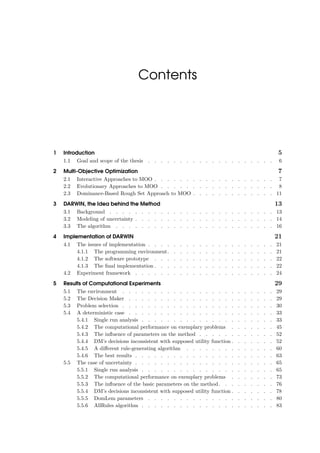
The interactive approach overcome this weaknesses by involving the DM in the process. A basic
structure of the approach is shown in Figure 2.1. At first, an initial set of solutions is generated.
It can be a subset of the Pareto-frontier or just a set of feasible solutions. Then, based on the
solutions, the Decision Maker specifies his or her preferences. It can be done by a systematic
dialog, asking a series of questions or asking the DM to indicate “good” solutions among the set.
From the DM’s answers a preference model is built. This additional preference information
guides the search towards a region indicated by the Decision Maker. This can save the computa-
tional cost, because the algorithm doesn’t have to go through the whole search space.
Again, new solutions, probably better fitted to the DM’s preferences are generated and the
algorithm shows them to him or her. If he or she finds it satisfactory (or a stop condition is met)
then the algorithm stops. Otherwise it advances to the next iteration.
There are several types of the IMO methods (consult [26] for an in-depth description):
• Trade-off based methods. A trade-off is an exchange, a price that one is willing to pay
(in form of lost on some of the criteria), in order to benefit on another criterion (or criteria).
These methods ask the DM questions about the trade-offs he or she can accept and then,
a preference model is inferred based on the tread-offs.](https://image.slidesharecdn.com/4981f33e-4e84-4fb8-a033-f832840408ae-161203112639/85/igor-kupczynski-msc-put-thesis-9-320.jpg)
![8 2 Multi-Objective Optimization
Generate an initial set
of solutions
Show the solutions to
the decision maker
Is any of the
solutions
satisfatory?
[Yes]
Ask the DM to indicate
"good" solutions
Extract preference
information
Improve the solution
set
[No]
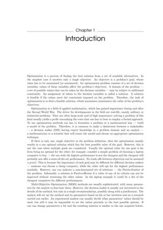
Figure 2.1: An activity diagram for a typical interactive process
• Reference point approaches — the DM specifies bounds on values of the objective func-
tions (i.e. reference points) and then, he or she can observe the effect of the bounds on the
generated solutions.
• Classification-based methods. It is not possible to improve a value of a goal of a solution
from the Pareto-frontier without worsening other goals of the solutions. In the classification-
based methods the DM is asked to select goals that can be impaired and the ones that he or
she wants to improve.
The interactive approach requires the Decision Maker’s collaboration during the process, how-
ever the approach offers strong benefits to justify this dedication. Clearly, the computational cost
required is lower than in other approaches, because there is no need to evaluate whole solution
space, just its small subset. The DM may not be able to express a global structure of his or her
preferences up front. It is also possible that his or her preferences will change along with the
change in understanding of the problem. During the interactive process the DM has an immediate
feedback — he or she may see how the decisions are affecting problem solutions.
One can say that solving a Multi-Objective Optimization problem is a constrictive process,
where the Decision Maker learns more about the problem — what kind of solutions are possible
and how his of her choices influences the results (see [26]). As a result, not only the most preferred
solution is given, but also the problem understanding by the DM is better.
2.2 Evolutionary Approaches to MOO
In 1859, Charles Darwin published his work “On the origin of species” [2]. He introduced a scientific
theory describing the evolution of species through the process called natural selection. According
to the theory, a trait can become less or more common in the population in dependence on its
effect upon the survival and reproduction of the individuals bearing the trait.](https://image.slidesharecdn.com/4981f33e-4e84-4fb8-a033-f832840408ae-161203112639/85/igor-kupczynski-msc-put-thesis-10-320.jpg)
![2.2 Evolutionary Approaches to MOO 9
P := Initialization
Termination
conditions are
met?
[Yes]
Evaluate(P) P' := Selection(P)
P'' := Variation(P')P := Elitism(P, P'')
[No]
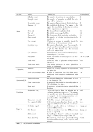
Figure 2.2: An evolutionary optimization procedure
This idea can be easily transfered to the optimization field. A solution to a problem — that
is, the set of values of problem’s decision variables — is a single individual in the population.
The problem is the environment — the higher the solution evaluation on a given problem, the
better it is fitted to the environment. A better fitness means higher chance that the traits of
a solution will be present in the next iteration (an analogue of a reproduction success rate). First
successful applications of the idea were done in the electrical engineering field (see [6]) and in the
fluid mechanics (see [29, 30]).
The main differences between the classical and the evolutionary optimization (EO) are (see [3]):
• Population-based. An EO procedure uses a population of solutions (a population ap-
proach), whereas the classical algorithms maintain one solution at a time (a point approach).
It enables an algorithm to maintain multiple optimal solutions, possibly from different parts
of the solution space. Unfortunately it rises the memory and computational footprint of an
EO algorithm.
• Stochastic operators. An EO procedure uses stochastic operators (e.g. selection, crossover
or mutation) instead of deterministic ones.
• Gradient information. An EO procedure does not usually use gradient information directly
in performing a search. This means that the procedure is immune to local optima in a search
space. However, the EO procedure may not be competitive with dedicated gradient approach.
The basic evolutionary optimization procedure is shown in Figure 2.2. The algorithm starts
with creating a population of solutions. Usually the population is created at random within
bounds of decision variables. Then a succesion of generations starts. The populations is updated
by a sequence of operators.
First, the population is evaluated. The evaluation means establishing an relative preference
order, that is sorting solutions from the best to the worst. After the evaluation the algorithm
chooses solutions to fill the mating pool. The better the solution the higher the probability to be
chosen. Then, the variation operator is being used. It is a series of steps, such as crossover or
mutation, generating a succeeding generation (an offspring) from parents in the mating pool. The
crossover ensures that parents’ traits will be present in the next generation while the mutation
acts as local search in the solution’s neighborhood. Finally, the elitism operator combines the old
population with the newly created offspring. Coping best solutions from the former ensures the
algorithm has a monotonically non-degrading value of the best solution.](https://image.slidesharecdn.com/4981f33e-4e84-4fb8-a033-f832840408ae-161203112639/85/igor-kupczynski-msc-put-thesis-11-320.jpg)
![10 2 Multi-Objective Optimization
100 1 2 3 4 5 6 7 8 9
10
0
1
2
3
4
5
6
7
8
9
Goal 1 (gain)
Goal2(gain) Pareto-frontier #1
Pareto-frontier
#2
Pareto-frontier#3
Pareto-frontier #4
The crowded areas
Individuals
Label
Figure 2.3: The NSGA-II evaluation
The choice of a fitness function is critical to the algorithm’s performance. In case of a problem
with a single criterion this is trivial — a value of the goal can be used. However, in the case
of the Multi-Objective Optimization, there are a number of objective functions to be optimized.
A possible approach to the problem is to use the dominance principle ([7]):
A solution x is said to dominate the other solution y, if both of the following conditions are
true:
1. The solution x is not worse than y on all objectives. Thus, the solutions are compared based
on their objective function values.
2. The solution x is strictly better than y on at least one objective.
All the solutions that are non-dominated by any other solution are forming the Pareto-frontier
of the problem.
According to [3] there are two ideal goals of the EMO:
1. Find a set of solutions which lies on the Pareto-optimal front, and
2. Find a set of solutions which is diverse enough to represent the entire range of the Pareto-
optimal front.
The most representative example of the Evolutionary Multi-objective Optimization (EMO)
algorithm is NSGA-II ([4]). The basic idea behind the algorithm is to assign each solution in
a population to a number of different Pareto-frontiers. All non-dominated individuals are assigned
to first Pareto-frontier and then removed from the population. All non-dominated individuals after
the removal are then assigned to second frontier. The process repeats until there are individuals in
the population. The lower the number of the frontier, which an individual belongs to, the higher
the fitness function for it. In case of a tie the crowding score is taken into account — the lesser the
crowd in the solution’s neighborhood in an objective space, the better the solution’s evaluation.
This is illustrated in Figure 2.3.](https://image.slidesharecdn.com/4981f33e-4e84-4fb8-a033-f832840408ae-161203112639/85/igor-kupczynski-msc-put-thesis-12-320.jpg)
![2.3 Dominance-Based Rough Set Approach to MOO 11
2.3 Dominance-Based Rough Set Approach to MOO
A rough set is an approximation of a conventional set — a pair of sets being a lower and an
upper approximation of the original set ([27]). The lower approximation is a set of all objects
that unambiguously can be classified as members of the target set. On the other hand, the upper
approximation is a set containing objects that cannot be unambiguously classified as members of
the complement of the target set. A boundary region is the part of solution space being part of
the upper approximation, but not the lower one.
Dominance-based Rough Set Approach (DRSA) is an extension of the rough set theory intro-
duced in [10, 11, 12]. The indiscernibility relation is replaced by the dominance relation (defined
in the former section). DRSA is applicable in the decision support field.
DRSA can model the situations in which a finite set of objects — vectors of values in the
decision variable space — has been classified to some decision classes, such that one object belongs
to exactly one class. The classes are preference ordered. The main task of DRSA is to structure
the classification into lower and upper approximations of unions of ordered decision classes, prior
to induction of monotonic decision rules, representing the preferences of an agent who made the
classification decision. An example of the DRSA data structuring is given in Figure 2.4.
The data in Dominance-based Rough Set Approach are often presented in a decision table. The
objects being considered are written in table rows, the decision attributes are table columns. The
last column is classification of the objects to a decision classes. A formal definition of the decision
table can be easily found in the literature. An example is given in Table 2.1.
On the basis of the table, decision rules may be induced. They are generalized description of
the knowledge represented in the table. A decision rule is a Horn clause (see [19]) in form of “if ...,
then ...”. The former part is called condition and the latter — consequent. The condition part
compares a value of an object attributes with given thresholds and the consequent part represents
the object classification if the condition part holds. Rules can be either certain — based on
objects from the lower approximation of the class, possible — based on objects from the upper
approximation and approximate — based on the boundary region. Each decision rule should be
minimal, i.e. cardinality of the set of conditions should be minimal.
Example rules generated from Table 2.1 are as follows:
1. If Literature ≥ good then Student ≥ good,
2. If Mathematics ≤ bad and Physic ≤ medium then Student ≤ bad,
3. If Mathematics ≥ medium then Student ≥ medium (possible).
DRSA can handle uncertainty and contradictions in the data, thus it can model a wide class
of real-world decision problems. For each rule r given in from Φ → Ψ, the following measures are
defined:
Student Mathematics Physics Literature Overall class
1 good medium bad bad
2 medium medium bad medium
3 medium medium medium medium
4 medium medium medium good
5 good medium good good
6 good good good good
7 bad medium medium bad
8 bad bad medium bad
Table 2.1: An example of the decision table](https://image.slidesharecdn.com/4981f33e-4e84-4fb8-a033-f832840408ae-161203112639/85/igor-kupczynski-msc-put-thesis-13-320.jpg)
![12 2 Multi-Objective Optimization
400 5 10 15 20 25 30 35
40
0
5
10
15
20
25
30
35
gain 2
gain1
Lower approximation of "High"
Upper approximation of "High"
High
Medium
Low
Figure 2.4: An example of the DRSA approach
• Support: supp(Φ, Ψ) = cardinality(||Φ ∧ Ψ||) — is the number of objects for which the
condition of the rule holds and the object classification is consistent with the consequent of
the rule.
• Confidence: confidence(Φ, Ψ) =
supp(Φ, Ψ)
cardinality(||Φ||)
— is the number of objects supporting the
rule in a relation to the number of objects for which the rule’s condition holds.
.
Objects supporting rule no. 3 are {S2, S3, S4, S5}, but the condition part holds also for S1.
The support is thus: supp(r3) = 4
5 = 0.8.
To induce all rules from the decision table one can use the All Rules algoritm (an optimized
version is described in [35]). Another option is to use the DomLem algorithm ([16]) generating
a minimal set of rules covering all the objects from a given table.](https://image.slidesharecdn.com/4981f33e-4e84-4fb8-a033-f832840408ae-161203112639/85/igor-kupczynski-msc-put-thesis-14-320.jpg)
![Chapter 3
DARWIN, the Idea behind the
Method
The basic idea of Darwin method was introduced in [14]. This idea will be described in the following
paragraph.
3.1 Background
The method combines two different approaches — Interactive Multi-Objective Optimization (IMO,
see 2.1) and Evolutionary Multi-Objective Optimization (EMO, see 2.2).
In the IMO paradigm one wants to elicit decision maker’s preferences by involving him or her
in the process. This is done by a systematic dialog with the decision maker (the DM). Questions
are being asked and the DM provides answers. Preference information is extracted on the basis of
these answers. Algorithm can then use the knowledge to produce solutions better fitted to his or
her preferences. The IMO framework is presented in Figure 2.1.
The rationale behind the interactive process is that the decision maker is interested only in
a small subset of preferred solutions or even in a single most preferred one.
This process makes it possible to gather preference information and then use this information
to construct better solutions. However, this is just a framework, so details are left up to the
analyst. One has to think particularly how to extract and store knowledge gathered on DM’s
answers and how to use this knowledge to generate and provide solutions better fitted to decision
maker’s preferences.
Human factor is yet another thing to consider. The DM is a human being and thus his or her
behavior may change. The challenge here is to find out what questions should be asked and how
often, as well as how many intermediate solutions should be presented to the DM for evaluation.
DARWIN is a realisation of the IMO process. It keeps generating solutions and improving them
on the basis of DM’s feedback. It only asks the DM to mark potentially good solutions, so that
only problem-domain knowledge is required; its user does not need to have expert knowledge in
the decision support field.
Evolutionary Multi-Objective Optimization (EMO) provides a computational engine for gener-
ating new, still better solutions in successive iterations — better in sense of an objective function
defined in the solution space. Most of the EMO methods are approximating Pareto-optimal front
by a set of solutions. So one solution is better than the other if the former Pareto-dominates the
latter. In case of two equivalent ones another factors have to be taken into account (for example
crowding score of NSGAII [4]). This is the case because if no preference information is given, all
Pareto-optimal solutions have to be considered equivalent.](https://image.slidesharecdn.com/4981f33e-4e84-4fb8-a033-f832840408ae-161203112639/85/igor-kupczynski-msc-put-thesis-15-320.jpg)
![14 3 DARWIN, the Idea behind the Method
100 1 2 3 4 5 6 7 8 9
10
0
1
2
3
4
5
6
7
8
9
Goal 1 (gain)
Goal2(gain)
Pareto-frontier
An area prefered by the DM
Dominated solutions
Figure 3.1: Pareto-front and area preferred by the decision maker
It seems natural to combine these two described approaches — Interactive Multi-Objective
Optimization and Evolutionary Multi-Objective Optimization. IMO is just a process framework
but still needs an engine to generate and improve solutions. EMO is such an engine. On the
other hand for EMO involving the decision maker in the procedure results in gathering preference
information. This information allows the procedure to focus on a specific region of Pareto-front —
the most relevant one to the decision maker. In this way IMO and EMO are complementing each
other.
This is important because of the “human factor”. If the number of solutions becomes huge, the
DM can not effectively analyze them and find the one that fits his/her preferences best, thus Pareto-
optimality is not sufficiently discriminative. However, guiding the search to preferred regions of the
solution space allows the method to converge faster to good solutions. It is shown in Figure 3.1.
DARWIN uses EMO procedure to improve generated solutions based on the DM’s preferences.
3.2 Modeling of uncertainty
It is often the case that not all numbers and coefficients are precisely known. It may be easier
for the decision maker to formulate the Multi-Objective Optimization problem giving the problem
coefficients in the form of intervals of possible values. For example, instead of saying that product
price will equal 20 units one can say it will be in the [19, 21] interval. In this situation the decision
maker is often interested in finding the best robust solution — that is good and possible in a large
part of uncertainty scenarios. DARWIN allows to give the coefficients in a form of intervals.
The set of all of the problem’s coefficients given as intervals and fixed on one of possible values
will be called scenario of imprecision (see Figure 3.2). If intervals are allowed, it is impossible to
calculate the exact value of problem’s objectives for given solutions. To handle this case all the
considered solutions are evaluated over a set of uncertainty scenarios.](https://image.slidesharecdn.com/4981f33e-4e84-4fb8-a033-f832840408ae-161203112639/85/igor-kupczynski-msc-put-thesis-16-320.jpg)
![10-1 0 1 2 3 4 5 6 7 8 9
a
b
c
Scenario: {a ->2, b -> 6, c -> 4}
a = [1, 10]
b = [5, 10]
c = [0, 5]
Figure 3.2: Scenario — set of intervals fixed on specific values
3.5-3.5 -3 -2 -1 0 1 2 3
0.1
0.2
0.3
0.4
25% 50% 75%
Figure 3.3: Percentiles of the normal distribution](https://image.slidesharecdn.com/4981f33e-4e84-4fb8-a033-f832840408ae-161203112639/85/igor-kupczynski-msc-put-thesis-17-320.jpg)
![16 3 DARWIN, the Idea behind the Method
Results of this evaluation are then aggregated to quantile space. The quantiles are points
taken at regular intervals from the cumulative distribution of a random variable. If the interval
consists of 0.01 of the distribution, then the quantiles are called percentiles (percentiles of the
normal distribution are shown in Figure 3.3). Instead of presenting all of the results, the method
calculates meaningful quantiles of results distribution for each objective. For example, percentiles
(like 1%, 25% and 50%) can be chosen. Percentiles divide ordered data into 100 of equally-sized
subsets — 1% percentile is the best of 1% worst solutions or alternatively the worst of 99% of the
best solutions.
Choice of these quantiles is connected with the DM’s attitude towards risk. If he or she wants to
avoid risk then his/her decision will be focused on quantiles from the beginning of the distribution
(e.g. 10%). On the other hand, when he or she is interested in the best possible solution even if
there is a risk involved, then the quantiles from the end of the distribution will be inspected (e.g.
75%).
In DARWIN the DM’s preferences are gathered and stored using DRSA methodology (see 2.3).
Dominance-Based Rough Set Approach is a framework for reasoning about partially inconsistent
preference data. DRSA already has successful applications in IMO area (see [10, 11, 12]).
DRSA will be applied in IMO process. After selecting “good” solutions from the provided set
the decision rules are induced to store the preferences. These rules are given in the form of “If ...
then ...”. Conditional part is a disjunction of conditions on attributes from quantile space. These
attributes are compared to specific values, e.g. profit25% >= 100 ∧ time1% <= 10. The consequent
part assigns a solution to a class (at least or at most), e.g. Class at least Good. So the whole rule
would be If profit25% >= 100 ∧ time1% <= 10 then Class at least Good.
3.3 The algorithm
DARWIN can operate on Multi-Objective Optimization (MOO) problems defined as follows:
[f1(x), f2(x), . . . , fk(x)] → max (3.1)
subject to:
g1(x) ≥ b1
g2(x) ≥ b2
. . .
gm(x) ≥ bm
(3.2)
Where:
x = [x1, x2, . . . , xn] is a vector of decision variables, called a solution;
f1(x), f2(x), . . . , fk(x) are objective functions, f : x → R;
g1(x), g2(x), . . . , gm(x) are constraint functions, f : x → R;
b1, b2, . . . , bm are real-valued right hand sides of the constraints.
It is possible to give some of the coefficients in objective functions or constraints in the form
of intervals (thus modeling ignorance — uncertainty about real value of a coefficient). A vector of
fixed values for each interval is called scenario of imprecision (see Figure 3.2).
DARWIN is composed of two nested loops — exterior and interior. The former is a realisation
of an interactive process and the latter is an EMO engine dedicated to improve solutions based on
the decision maker’s preferences. This is illustrated in Figure 3.4.
The exterior loop algorithm, corresponding to the IMO interactive process is shown on alg. 1.
A More detailed description of each step follows.
First, one has to generate a set of feasible solutions to the MOO problem first. This can be
done using the Monte Carlo method. The Monte Carlo concept itself is not new. A concept of](https://image.slidesharecdn.com/4981f33e-4e84-4fb8-a033-f832840408ae-161203112639/85/igor-kupczynski-msc-put-thesis-18-320.jpg)
![Generate an initial set
of solutions
Show the solutions to
the decision maker
Is any of the
solutions
satisfactory?
[Yes]
[No]
Generate an initial set
of scenarios
Ask the DM to indicate
a subset of "good"
solutions
Generate rules
Perform an
evolutionary
optimization
Figure 3.4: Activity diagram for DARWIN. “Perform an evolutionary optimization” step is
forming the interior loop
Algorithm 1 DARWIN’s exterior loop
1: X ← GenerateSolutions
2: S ← GenerateScenarios
3: loop
4: for all x ∈ X, s ∈ S do Evaluate each solution over all of the scenarios
5: Evaluate(x, s)
6: end for
7: isSatisfied ← PresentResults
8: if isSatisfied then
9: stop
10: else
11: X ← AskToMarkGood(X)
12: end if
13: rules ← InduceDecisionRules(X)
14: X ← EmoProcedure(rules) the interior loop
15: end loop](https://image.slidesharecdn.com/4981f33e-4e84-4fb8-a033-f832840408ae-161203112639/85/igor-kupczynski-msc-put-thesis-19-320.jpg)
![18 3 DARWIN, the Idea behind the Method
statistical sampling became popular after digital computing machines had been invented (see [25]).
This method can be described as random sampling a domain of a problem. In the most basic
variant one can just pick a solution at random and check if it is feasible. Unfortunately, it will be
impossible unless the non-feasible space is only a small part of the domain. Additional hints for
the generator, for example in the form of analyst’s suggestions, can be taken into account.
At this stage goals and constraints are allowed to contain intervals corresponding to the un-
certainty of a model. Thus a set of scenarios needs to be generated. Each of these scenarios is
a realisation of the problem with fixed values of the intervals. It is worth noting that if the problem
constraints are given in an uncertain form — that is containing coefficients in the form of intervals
— it could be impossible to determine whether a given solution is possible. If that is the case, then
lines 1 and 2 should be swapped and feasibility of a solution set should be checked on generated
scenarios.
In lines 4 to 6 each solution if evaluated over each scenario. Results of this evaluation phase
are then gathered and presented to the decision maker in 7. The DM is a human being though,
so in order to get valuable feedback one need to show the data in aggregated form. The au-
thors proposed a meaningful quantiles to be presented. For example f1%
1 (x), f25%
1 (x), f50%
1 (x),
. . . , f1%
k (x), f25%
k (x), f50%
k (x) for all x ∈ X.
If the DM finds solution in the set of presented ones satisfactorily, then the problem is solved
and algorithm ends here. If not, however, he or she is asked to indicated the “good” solutions
in the set (line 11). On the basis of this distinction, the method generates a set of decision rules
(line 13). These rules are then passed to the interior loop (line 14) where — by using the EMO
paradigm (see 2.2) — DARWIN performs search of the solution space. The search is driven towards
a specific region on the basis of the rules. Finally new solutions, better fitted to DM’s expectations
are generated and the process starts over again.
Algorithm 2 shows the interior loop of DARWIN method. This loop is an EMO procedure
guided by the decision rules induced in exterior loop on DM’s selections.
Algorithm 2 DARWIN’s interior loop
1: procedure EmoProcedure(rules)
2: X ← GenerateSolutions
3: S ← GenerateScenarios
4: loop
5: for all x ∈ X, s ∈ S do this loop calculates meaningful quantiles for each solution
6: Evaluate(x, s)
7: end for
8: if termination conditions fulfilled then
9: return X
10: end if
11: pScore ← CalculatePrimaryScore(X)
12: sScore ← CalculateSecondaryScore(X)
13: X ← RankSolutions(X, pScore, sScore)
14: P ← SelectParents(X )
15: O ← RecombineOffspring(P)
16: O ← Mutate(O)
17: X ← MergePopulations(X , O )
18: end loop
19: end procedure
The procedure starts by generating a new set of feasible solutions and possible scenarios in
lines 2, 3. Then in line 4 actual evolutionary optimization starts.
Each solution is an individual. The solution set constitutes a population. Iterations of a loop
defined in line 4 mark generations of the population. Termination condition could be for example
a fixed number of iterations or a fixed amount of time.](https://image.slidesharecdn.com/4981f33e-4e84-4fb8-a033-f832840408ae-161203112639/85/igor-kupczynski-msc-put-thesis-20-320.jpg)
![3.3 The algorithm 19
First, in every generation the population is evaluated and ranked. The process starts with
evaluation of each solution over every scenario (5 – 7). After the evaluation meaningful quantiles
are known for each solution. Then the procedure can calculate a primary score for each of the
individuals. The primary score is computed as follows. Let:
rules(x) = {ruleh ∈ rules : ruleh is matched by solution x}
rules(x) is a set of rules (ruleh ∈ rules) matched by solution x ∈ X.
X(ruleh) = {x ∈ X : x is matching ruleh}
For each ruleh ∈ rules : X(ruleh) is a set of solutions matching this rule.
w(ruleh) = (1 − δ)card(X(ruleh))
Each rule (ruleh) gets a weight related to the number of times it is matched by a solution.
δ is a decay of rule weight. For example δ = 0.1. This formula associates higher weight for
rules matching lesser number of solutions — this is an important property because it allows
to maintain diversity with respect to rules.
PrimaryScore(x) = ruleh∈rules(x) w(ruleh)
Finally PrimaryScore(x) is a primary score of a given solution (x ∈ X).
In case of a draw also a secondary score is considered for each solution. This score is calculated
similarly to a crowding distance score in NSGA-II method ([4]). The difference lies in the fact,
that this score is calculated in a quantile space instead of original objective space, e.g. f1%
1 ×
f25%
1 × f50%
1 × · · · × f1%
k × f25%
k × f50%
k . The procedure is shown in alg. 3.
Algorithm 3 Procedure calculating crowding distance
1: procedure CalculateCrowdingDistance(X)
2: n ← |X| Number of solutions
3: for all x ∈ X do Initialize
4: distance(x) = 0
5: end for
6: for all o ∈ objectives do
7: X ← Sort(X, o) Sort solutions using value of an o objective
8: distance(X‘(1)) ← ∞ Boundary solutions get highest score possible
9: distance(X‘(n)) ← ∞ X‘(n) is the n-th element of the X‘ ordered set
10: end for
11: for i ← 2, n − 2 do o(x), x ∈ X is a value of the objective o in the solution s
12: distance(X‘(i)) ← distance(X‘(i)) +[o(X‘(i − 1)) + o(X‘(i − 1))]
13: end for
14: end procedure
In line 14 parents selection is done. The process is a Monte Carlo procedure; possibility of
selecting a solution x ∈ X as a parent is:
Pr(x) =
|X| − rank(x) + 1
|X|
γ
−
|X| − rank(x)
|X|
γ
where rank(x) is a rank of a solution x ∈ X in the ranking made in line 13. γ ≥ 1 is an elitism
coefficient. The higher the γ, the bigger the probability of selecting a high-ranked solution as
a parent.
In line 15 a new individual (a child) is created using two of the parents chosen in the previous
step — a ∈ P, b ∈ P. The child is obtained by combining the parents together:
z = λa + (1 − λ)b
λ is a random real-valued number; 0 ≤ λ ≤ 1.](https://image.slidesharecdn.com/4981f33e-4e84-4fb8-a033-f832840408ae-161203112639/85/igor-kupczynski-msc-put-thesis-21-320.jpg)

![Chapter 4
Implementation of DARWIN
DARWIN is a high-level description of an algorithm that can be used to solve a multi-objective
optimization problem. It is a list of steps to execute and calculations to perform. Therefore,
one does not need a computer to realize the decision-making process. However, in practice it is
almost impossible to complete all the steps without a dedicated software application. Moreover,
to evaluate the method’s performance one needs to repeat the experiments several times.
For the reasons stated above it was required to implement the method as a computer pro-
gram. This chapter describes technologies used for the DARWIN’s implementation, as well as an
experiment framework development.
4.1 The issues of implementation
4.1.1 The programming environment
The environment in which DARWIN has to function is not empty; thus it has to be taken into
account during the development of the implementation. DARWIN is a realization of an interactive
process, therefore a way of communication with the decision maker is required. Another restriction
is imposed by the need of inducing decision rules from the DM’s evaluated examples of solutions.
The decision maker has to provide a problem he or she wants to solve. It can be done in a model
file. If one wants to change the default parameters’ values, then a configuration file with the values
is also required. Moreover, during the algorithm’s run, presence of the decision maker is needed
in order to select “good” solutions from the provided ones. Consult the user manual (6) for more
details on the file formats. The parameters are described later in this section.
Decision rules store the DM’s preferences, therefore they are a symbolic representation of trade-
offs he or she is willing to make, as well as the importance of each criterion. They ensure robustness
of the resulting solutions because of an underlying DRSA framework. The rules are a very im-
portant part of the method. Thus, a way — an algorithm — to generate them is needed. In the
method’s description provided in [13, 15, 9], a phase of obtaining the rules is treated as a black
box. It is assumed that a component able to generate rules from the DM’s selection exists. Details
are omitted — it is up to an analyst (or to a developer of an implementation) to use a software
component he or she finds feasible.
The implementation of the DRSA framework, being able to induce decision rules from a given set
of examples is a complex task, both in terms of possible technical challenges as well as conceptual
and scientific work that needs to be carried out. Such a software application deserves a paper
of its own. Therefore, the author decided to use an existing implementation in order to focus
on the DARWIN method. Java Rough Set (jRS) — a project carried out at the Laboratory of
Intelligent Decision Support Systems at Pozna´n University of Technology that aims at providing](https://image.slidesharecdn.com/4981f33e-4e84-4fb8-a033-f832840408ae-161203112639/85/igor-kupczynski-msc-put-thesis-23-320.jpg)
![22 4 Implementation of DARWIN
DRSA framework implementation in Java — was chosen. It contains the DomLem algorithm [16]
able to generate a minimal set of decision rules from the examples given as its input.
jRS is written in Java programming language1
and runs on top of the Java Virtual Machine
(JVM [23]). The JVM is a portable platform capable of running the Java bytecode. Having a Java
component (jRS in this case) effectively put a constraint on the DARWIN implementation — it is
required that the implementation is also delivered as a JVM application. However, the technical
details of the Java platform are out-of-scope of this paper, so they are omitted unless relevant for
the DARWIN’s description.
Unfortunately, generating only a minimal set of rules may not be sufficient. The primary score
in the interior loop is based on a number of rules matching a given solution. Therefore, having
more rules may prevent a gradient loss in the evolutionary optimization. To check if this effect has
serious impact on the performance, another rule-generating algorithm was developed. The author
implemented AllRules algorithm [17] in Scala programming language. Again, the algorithm’s
details are out of the scope of this paper. Nevertheless, it is worth noting that the number of rules
generated by AllRules is greater than the one generated by DomLem.
4.1.2 The software prototype
As his first task, the author chose to implement a prototype of the program. The goal was to check
the behavior of the method — if it works, converges to the preferred region, is able to generate
a reasonable solution and to withstand the uncertainty in the decision maker’s preferences; to find
out if the overview given in [13, 15, 9] is accurate enough to develop a working software. More
important however, was to identify potential problems and to gain a deep knowledge of the method.
The prototype was developed in Java. Java is a very popular language and de facto an industry
standard in many fields, especially in enterprise applications. The application itself is able to solve
a subset of the MMO problems. It supports uncertainty and it simulates the decision maker. It is
a working implementation of the method. The goal was achieved — to develop a working piece of
software showing that DARWIN is able to solve multi-objective optimization problems.
Unfortunately, the prototype has not been fully featured. It has contained only a simulated
DM and lacked any user interface at all. The problem to solve and the DARWIN parameters are
hard-coded for the prototype. Nevertheless, the code was being developed in an extensible way
and contained a suite of unit tests. However, it is a common practice in the software engineering
to discard the prototype and start developing the final application from scratch. This was the
case with DARWIN — the author’s knowledge of the method changed during the prototyping and
starting from the beginning has been considered a better option.
4.1.3 The final implementation
The Java language is stable, well-tested and features numerous libraries dedicated to almost every
possible applications; unfortunately, it is also very verbose and lacks support for many of the recent
trends in the computer programming and software development. It is a great tool for large teams,
as it is usually the case in the enterprise application market. However, what is a good solution for
a team is not essentially the best possible tool for a single developer working on a project.
The author decided to develop the implementation in Scala2
. Scala is a multi-paradigm pro-
gramming language combining object-oriented features with functional programming. The former
paradigm is a dominant contemporary software development practice; it allows to program and
model problem domain’s objects as well as any relations between them. However, the latter makes
it possible to write a concise code dealing with mathematical computations. This is a very useful
trait in scientific applications.
1Developer Resources for Java Technology — http://www.oracle.com/technetwork/java/index.html
2The Scala Programming Language — http://www.scala-lang.org/](https://image.slidesharecdn.com/4981f33e-4e84-4fb8-a033-f832840408ae-161203112639/85/igor-kupczynski-msc-put-thesis-24-320.jpg)
![4.1 The issues of implementation 23
Scala runs on JVM, therefore it is compatible with existing Java libraries. The Scala compiler
produces the Java bytecode from a Scala source code. The bytecode is nearly identical to the one
generated from a Java source. The only difference is that Scala programs require the presence of
an additional run-time library — scala-library.jar. The language was designed by Martin Odersky
and started as a project in ´Ecole Polytechnique F´ed´erale de Lausanne (EPFL). Because of the
functional elements and different syntax Scala programs are usually shorter and easier to read
than their Java counterparts, especially when dealing with mathematical operations.
The DARWIN code is divided into packages. Their structure is shown in Figure 4.1. Their de-
scription follows. pl.poznan.put.darwin is a root package following Java naming conventions [21].
For readability its name is omitted in the following description. Packages:
evolution — a module containing classes responsible for the evolution of solutions. It con-
tains a controller driving the process, an engine of the evolutionary algorithm, evolutionary
operators (mutation and cross-over) and a parent selection strategy.
jrsintegration — an abstraction layer over the DRSA framework. This module contains classes
responsible for integration with jRS and DomLem algorithm. They are able to convert
DARWIN’s solutions to a format required by the jRS, invoke the DomLem algorithm and
later — during the interior loop — check if a given solution matches any of the generated
rules.
model — models a hierarchy of objects for an abstract MOO problem. Contains basic classes
required to represent a problem, its variables, goals and constraints, as well as classes rep-
resenting a solution and a scenario of uncertainty. A problem parser — for reading problem
instances from files, a solution evaluator — computing a value of solution against given sce-
narios and a configuration reader — setting DARWIN’s options on the basis of a file, are also
components of the model package.
simulation — a package responsible for connecting all the other parts together. It initializes
the process by asking model to read the problem and the configuration; takes care of the
interaction with the DM, invokes jrsintegration to process the preferences and to obtain
the rules and finally interacts with the evolution controller from the evolution package. It
can also simulate the decision maker and generate reports if needed for automated experiment
framework.
utils — additional utility classes for the other modules.
In order to reduce the number of bugs and eliminate recurring of the fixed bugs an extensive
allrules darwin
evolution gui jrsintegration model
problem solution
simulation utils
pl.poznan.put
Figure 4.1: The package structure of DARWIN](https://image.slidesharecdn.com/4981f33e-4e84-4fb8-a033-f832840408ae-161203112639/85/igor-kupczynski-msc-put-thesis-25-320.jpg)
![24 4 Implementation of DARWIN
test suite accompanies each of the packages. In order to streamline the building process the Scala
Build Tool (SBT, see [18]) is used to manage dependencies, to take care of running the test suite
and to build the application from its source code. The code contains javadoc3
on most of the API
methods and a lot of comments in places that could be particularly hard or tricky to understand.
Therefore it should be possible for the other developer to use and extend the code delivered as
a part of the thesis. A manual for the end-user is enclosed at the end of the paper.
A lot of DARWIN parameters are mentioned throughout the paper. They are gathered and
described in Table 4.1. The parameters can be set in a configuration file. The options are split
into sections and listed in the table. The syntax of the configuration file is described in the user
manual (6).
4.2 Experiment framework
One of the goals of the thesis was to evaluate the DARWIN’s performance and the importance
of the parameters. To do this a set of tools was developed. Firstly, DARWIN can be instructed
to log details of an execution to a file (see Table 4.1). These logs consist of two reports — the
evolution report and the DM’s decisions report. The former contains the information about the
population’s shape and the latter about the decisions made by the decision maker. The reports
are in the comma separated values format (CSV [31]).
The algorithm is interactive which means that constant human supervision is required. How-
ever, one needs to repeat the experiments over and over again. For this reason the decision maker
has been simulated. It is possible to pass a utility function for a supposed decision maker and
then, the algorithm will make a decision on its own on the supposed utility basis. This automates
a single run of DARWIN, however an operator is still required to start the program over and, if
necessary, to change the execution parameters.
To bypass this limit and streamline the process, the experiment framework is provided. One
can define a base configuration along with a test plan and then a computer will proceed with an
execution of the test plan. Scripts composing the framework are written in Python — a general,
high-level programming language4
and glued together using the Bash shell scripts5
. A description
on how to use the framework is provided as a part of the user manual 6.
A test plan execution will typically result in a number of report files full of the runs’ details.
It would be a tremendous task to analyze them by hand. However, presenting this data in an
aggregated form as a set of charts can immensely simplify the analysis.
R is an environment for statistical computing6
. The program along with ggplot library (see [32])
has been used for the automatic chart generation. The R scripts can import the CSV reports,
aggregate and process the data and finally generate a chart.
First, a user prepares a test plan and sends it to the framework. The framework is repeatedly
running DARWIN with a simulated decision maker. Resulting reports are then processed by the
R scripts. As a result charts are generated.
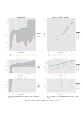
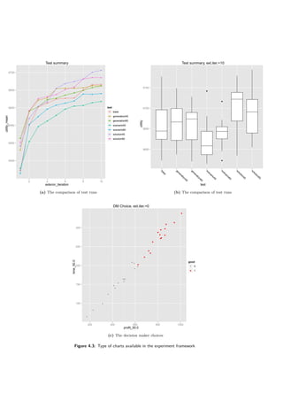
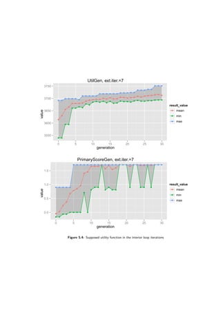
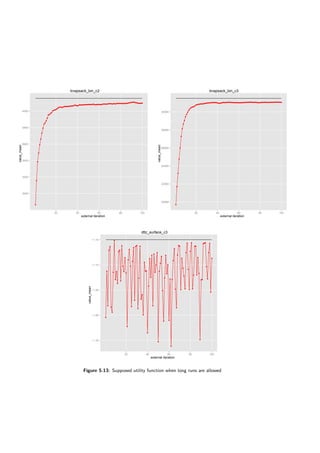
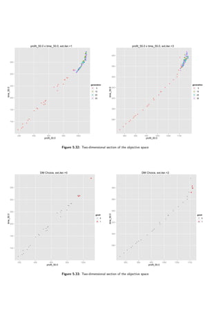
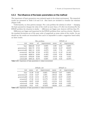
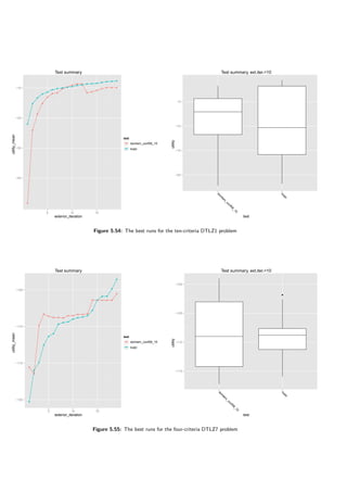
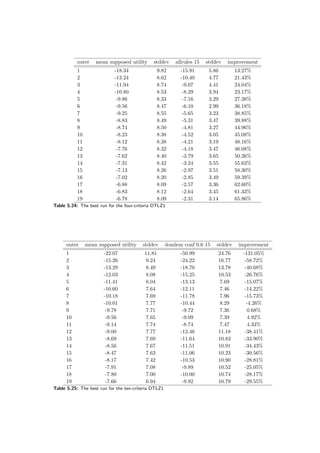
It is possible to generate the following type of charts (they are shown in Figure 4.2 and 4.3).
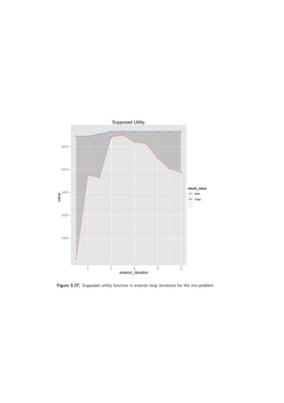
• A change of the supposed utility value during the exterior loop iterations. Example shown
in Figure 4.2a. This is a basic chart for the analysis, because it shows a high-level overview
of the run from the decision maker’s perspective.
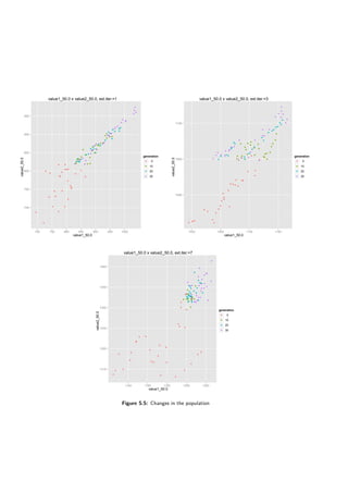
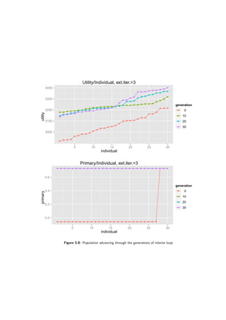
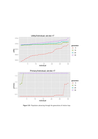
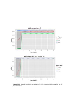
• A change in a population shape during the interior loop run. May show a convergence of
a population to a specific region. Figure 4.2b.
3Javadoc Tool — http://www.oracle.com/technetwork/java/javase/documentation/index-jsp-135444.html
4The Python Programming Language — http://python.org/
5Bourne-Again SHell — http://www.gnu.org/software/bash/bash.html
6The R Project for Statistical Computing — http://www.r-project.org/](https://image.slidesharecdn.com/4981f33e-4e84-4fb8-a033-f832840408ae-161203112639/85/igor-kupczynski-msc-put-thesis-26-320.jpg)

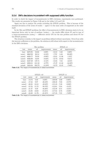
![30 5 Results of Computational Experiments
Unfortunately real decision maker, being a human isn’t as predictable and repeatable as the
described process. In the sections 5.4.4 and 5.5.4 the results of introducing inconsistencies to DM’s
decisions are presented.
In the following problems the supposed utility function is also defined.
5.3 Problem selection
The area of interest for Multi-Objective Optimization is huge and consists of many potential prob-
lems to be solved. There are multi-criteria versions of classical problems, like minimum spanning
tree [8], traveling salesman problem (TSP) [1] or knapsack problem [28] as well as an artificially
generated ones — like the DTLZ problem [5] Some of them are interesting because of their real-life
applications while the others are good for experimenting and testing purposes.
It is worth noting that the ordinary single-criterion versions of the problems can be easy to
solve. However, in multi-criteria settings one has to infer the decision maker’s preferences and
approximate the supposed utility function correctly. The challenge here is not to build the best
optimization algorithm for all the problems (this is impossible according to no-free-lunch theo-
rem [34]) but rather a framework for preference information extraction.
The experiments were performed using following problems:
Two-criteria binary knapsack problem
¯x = [x1, x2, . . . , x300]
xi ∈ {0, 1}; i = 1, 2, . . . , 300
max value1: ¯a1 · ¯x
max value2: ¯a2 · ¯x
subject to:
weight: ¯w · ¯x ≤ b
(max) supposed utility:
1 ∗ value1 + 2 ∗ value2
Where ¯x is a vector of items to be chosen. The problem is binary, so each xi ∈ ¯x can be
either selected (xi = 1) or not(xi = 0). There are two-criteria: value1 and value2. Each one
is a sum of items multiplied by associated weights (vector ¯a1 and ¯a2).
Knapsack constraint is given. One can choose items up to a certain weight (b). There is
a vector of weights associated with each item ( ¯w). The limit is defined that it is possible to
choose about 2/3 of the items.
Weights ( ¯a1, ¯a2, ¯w) are uniformly distributed vectors of values in [0, 10) interval.
Two-criteria continuous knapsack problem
¯x = [x1, x2, . . . , x300]
xi ∈ [0, 1); i = 1, 2, . . . , 300
max value1: ¯a1 · ¯x
max value2: ¯a2 · ¯x
subject to:
weight: ¯w · ¯x ≤ b
(max) supposed utility:
3 ∗ value1 − 1 ∗ value2](https://image.slidesharecdn.com/4981f33e-4e84-4fb8-a033-f832840408ae-161203112639/85/igor-kupczynski-msc-put-thesis-32-320.jpg)
![5.3 Problem selection 31
Continuous version of the knapsack problem. Description given for the binary version also
applies here. The only difference is that now the items can be partially selected (∀xi∈¯xxi ∈
[0, 1)).
Three-criteria binary knapsack problem
¯x = [x1, x2, . . . , x300]
xi ∈ {0, 1}; i = 1, 2, . . . , 300
max value1: ¯a1 · ¯x
max value2: ¯a2 · ¯x
max value3: ¯a3 · ¯x
subject to:
weight: ¯w · ¯x ≤ b
(max) supposed utility:
1 ∗ value1 − 1 ∗ value2 + 2 ∗ value22
Two-criteria problems can be easily visualized and analyzed. However, in real-life applications
there is often a need for three or more criteria. There is a leap in moving from two- to
multiple-criteria, so it is worth comparing the results achieved on the three-criteria knapsack
problem with its two-criteria counterpart.
Three-criteria DTLZ problem generated using constraint surface approach
min f1: x1
min f2: x2
min f3: x3
subject to:
0 ≤ xi ≤ 1, i = 1, 2, 3
− x1 + x2 + 0.6 ≥ 0
x1 + x3 − 0.5 ≥ 0
x1 + x2 + x3 − 1.1 ≥ 0
(max) supposed utility:
− 1 ∗ f1 − 2 ∗ f2 − 1 ∗ f3
This problem consists of three simple linear criteria. The solution space is a three-dimensional
cube bounded by the 0 ≤ xi ≤ 1 constraint. To make the problem challenging parts of the
solution space are being cut off by additional constraints.
This problem was build according to constraint surface approach presented in [5].](https://image.slidesharecdn.com/4981f33e-4e84-4fb8-a033-f832840408ae-161203112639/85/igor-kupczynski-msc-put-thesis-33-320.jpg)
![32 5 Results of Computational Experiments
Two-criteria robust mix problem
max profit: pAmin(xA, dA) + pBmin(xB, dB) + pCmin(xC, dC)
− (r1
AxA + r1
BxB + r1
CxC)p1
R − (r2
AxA + r2
BxB + r2
CxC)p2
R
min time: tAxA + tBxB + tCxC
where:
pA ∈ [20, 24], pB ∈ [30, 36], pC ∈ [25, 30]
dA ∈ [10, 12], dB ∈ [20, 24], dC ∈ [10, 12]
r1
A ∈ [1, 1.2], r1
B ∈ [2, 2.4], r1
C ∈ [0.75, 0.9]
r2
A ∈ [0, 5, 0.6], r2
B ∈ [1, 1.2], r2
C ∈ [0.5, 0.6]
p1
R ∈ [6, 7.2], p2
R ∈ [9, 9.6]
tA ∈ [5, 6], tB ∈ [8, 9.6], tC ∈ [10, 12]
subject to:
0 ≤ xA ≤ 12
0 ≤ xB ≤ 24
0 ≤ xC ≤ 12
(max) supposed utility:
profit1%
+ 3 ∗ profit25%
+ 2 ∗ profit50%
− time1%
− 3 ∗ time25%
− 2 ∗ time50%
The problem was described in a presentation DARWIN: Dominance-based rough set Approach
to handling Robust Winning solutions in INteractive multiobjective optimization given at 5th
International Workshop on Preferences and Decisions in Trento, 2009) describing the DAR-
WIN method. It contains a lot of coefficients given in the form of intervals. For readability’s
sake they were named and defined below the criteria.
The goal is to set quantity of each product (A, B, C) to be produced. One wants to maximize
the profit and minimized the total time it takes to produce the products. pi is the price of
a product i ∈ {A, B, C} on the market. There is also maximal demand the market can
consume (di). Each product consists of two raw materials — r1 and r2. Quantity needed
to produce i-th product is defined (r1
i , r2
i ) as well as the product price (p1
R, p2
R). Finally, it
takes time to produce a given product — tA, tB, tC.
Coefficients are given in the form of intervals, so each solution has to be evaluated on many
scenarios of uncertainty. This is why no exact values are used in the supposed utility function
— one can not do it because there are no exact values, only a series of evaluation results.
Percentiles are used instead. goal25%
means a result of the best evaluation among the worst
25% of evaluations.](https://image.slidesharecdn.com/4981f33e-4e84-4fb8-a033-f832840408ae-161203112639/85/igor-kupczynski-msc-put-thesis-34-320.jpg)
![5.4 A deterministic case 33
Four-criteria robust DTLZ7 problem
min fj(x): 0.1 ∗
10j
10(j−1)+1
xi + [0, 2 ∗ (4 − j)], j = 1, 2, 3, 4
subject to:
g1(x): f4(x) + 4f1(x) − 1 ≥ 0
g2(x): f4(x) + 4f2(x) − 1 ≥ 0
g3(x): f4(x) + 4f3(x) − 1 ≥ 0
g3(x): 2 ∗ f4(x) + min[f1(x) + f2(x), f1(x) + f3(x), f2(x) + f3(x)] − 1 ≥ 0
0 ≤ xi ≤ 1, i = 1, 2, 3, 4
(max) supposed utility:
− 4 ∗ f60%
1 − 3 ∗ f60%
2 − 2 ∗ f60%
3 − 1 ∗ f60%
1 − 8 ∗ f30%
1 − 6 ∗ f30%
2 − 4 ∗ f30%
3 − 2 ∗ f30%
1
This problem is a variation of DTLZ7 problem from [5] article. The problem was constructed
using constraint surface approach described in the article. However, interval coefficients were
added to the goals.
Robust DTLZ1 problem
min f1(x): [0.3, 0.7] ∗ x1x2 . . . xM−1(1 + g(xM ))
min f2(x): [0.3, 0.7] ∗ x1x2 . . . (1 − xM−1)(1 + g(xM ))
. . .
min fM−1(x): [0.3, 0.7] ∗ x1(1 − x2)(1 + g(xM ))
min fM (x): [0.3, 0.7] ∗ (1 − x1)(1 + g(xM ))
where:
g(x) = 100 ∗ (5 +
M+4
i=M
[(xi − 0.5)2
− cos(20π(xi − 0.5))])
n = M + 4
subject to:
0 ≤ xi ≤ 1, i = 1, 2, . . . n
(max) supposed utility:
M
i=1
(−M + i − 1) ∗ f25%
i
Another problem that is suggested in [5]. It was constructed using bottom-up approach. In-
tervals were added to the goal functions. M indicates the number of goals. In the experiments
problems with 4 and 10 criteria were used.
5.4 A deterministic case
5.4.1 Single run analysis
In order to observe the algorithm’s behavior a detailed analysis of a single run is presented in this
section. The problem being analyzed is the two-criteria binary knapsack problem. The problem
is simple and the number of criteria small in order to focus on the algorithm. Moreover, no
uncertainty in the form of interval coefficients is considered.](https://image.slidesharecdn.com/4981f33e-4e84-4fb8-a033-f832840408ae-161203112639/85/igor-kupczynski-msc-put-thesis-35-320.jpg)
![5.4 A deterministic case 45
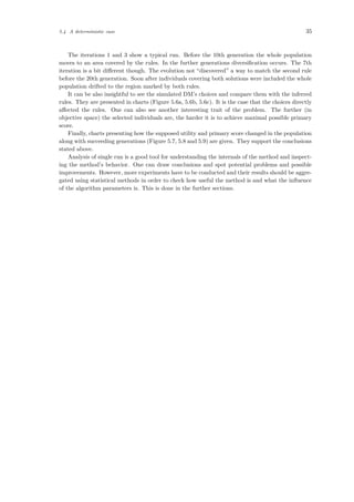
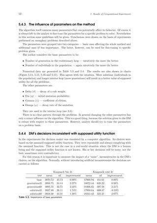
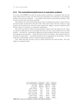
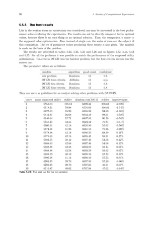
5.4.2 The computational performance on exemplary problems
It is important to know what performance can be expected from an algorithm. When no uncertainty
is considered in a problem and one assumes the supposed utility function, then it is easy to get the
optimal solution using linear programming solver. Of course in real-world applications the supposed
utility function is not known a priori. One can test this algorithm in such an artificially created
environment and then assume that the behavior will resemble the one in real-world problems.
Results of the evaluation on the following problems are given:
• Two-criteria binary knapsack problem, optimal value = 4154.441453.
• Two-criteria continuous knapsack problem, optimal value = 32700.41689.
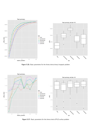
• Three-criteria binary knapsack problem, optimal value = 31502.10927.
• Three-criteria DTLZ problem generated using constraint surface approach, optimal value
= −1.1.
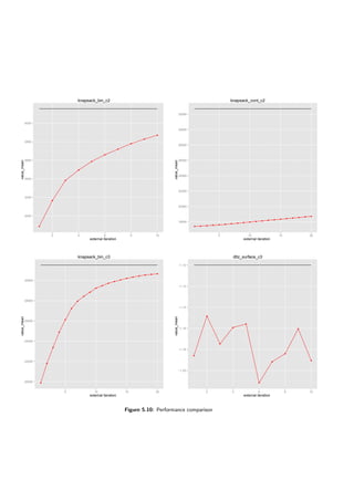
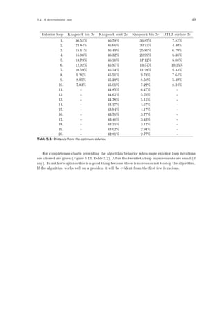
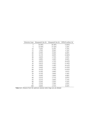
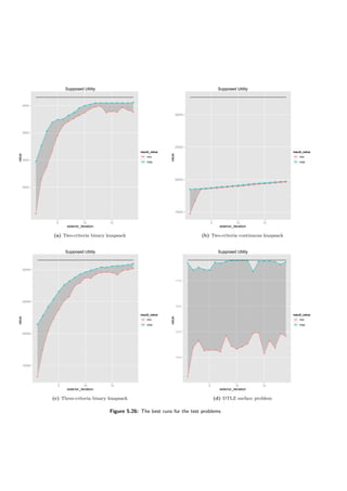
The tests were repeated at least fifteen times and the results averaged. They are presented in
Figure 5.10 and Table 5.1. Depending on a problem 10 or 20 iterations of the exterior loop were
simulated. Normally it would be up to the DM to stop when he or she is satisfied with the solution.
However, one can safely assume that if no satisfactory solution is found up to the 10th iteration,
the decision maker will not want to investigate the problem with this method any further.
On both binary knapsack problems the performance is very good — they are not further than
10% away from the optimal solution after the 10th iteration. The same is true for the surface
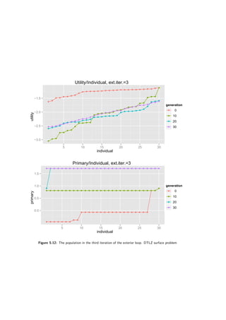
problem. However, looking at the Figure 5.10d one can see a bizarre phenomenon — the supposed
utility is falling down in a few runs.
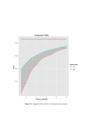
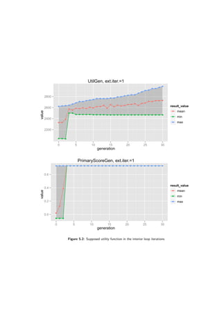
On the other hand, the evolutionary algorithm knows nothing about the utility function so
it may happen. The chart (Figure 5.10d) was generated using aggregated (averaged) results,
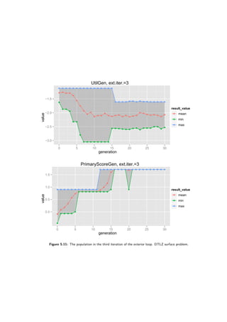
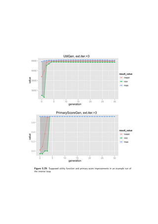
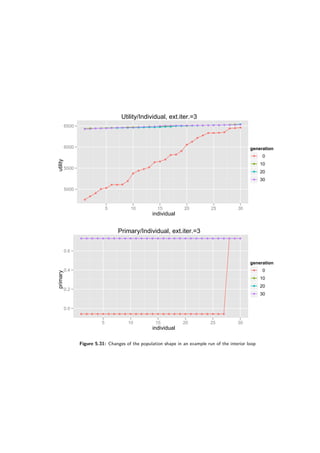
however this happened in most of the runs. To give a further insight charts showing evolution in
a third exterior loop are presented (not that the charts are for a single run only, not aggregated).
The charts are in figures 5.11 and 5.12. As one can see the evolutionary algorithm improves the
population from its perspective (the primary score factor). However, supposed utility function is
being lowered in the process.
This is the case because generated decision rules:
1. f1 ≤ 0.14033 ⇒ class ≥ GOOD
2. f3 ≤ 0.56462 ⇒ class ≥ GOOD
are not selective enough. It is possible that switching DomLem to another algorithm — generating
all possible rules instead of a minimal set would help here. Still the results achieved by the
DARWIN method are good on this problem.
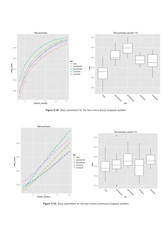
On the contrary, continuous knapsack problem performs extremely poor — only 55% of the
optimum after the 10th run and 58%, so almost no improvement, after the 20th. Investigating
single runs at length provided no more details. The problem lies in the evolutionary algorithm,
more precisely in its crossover operator. In the DARWIN method a from of the distance preserving
crossover is used. The form where a child is somewhere in between its parents. However, in
continuous variant it is usually the case to take items one-by-one starting with the one with the
greatest value per unit until the weight constraint is reached.
Considering the constraints (∀xi∈items : 0 ≤ xi ≤ 1) — most of the individuals will have their
decision variables in the form of xi ≈ 0.5 after a few generations. But for the optimal solutions
most of the variables take either 1 or 0. That is why improvement is happening so slowly here.
Relying on the author’s intuition changing the crossover operator would solve the problem with
continuous knapsack. Choosing the right operator for a given problem is a well-known subject in
the multi-objective optimization ([3]). However, it is out-of-scope of this paper.](https://image.slidesharecdn.com/4981f33e-4e84-4fb8-a033-f832840408ae-161203112639/85/igor-kupczynski-msc-put-thesis-47-320.jpg)
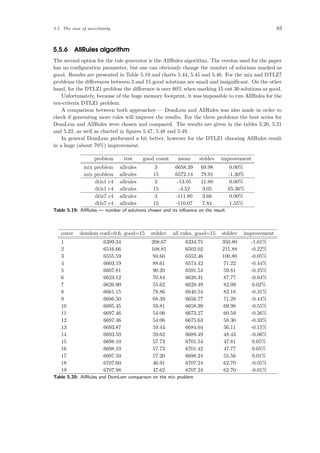
![56 5 Results of Computational Experiments
Knapsack bin 3c DTLZ surface 3c
test mean sd improvement mean sd improvement
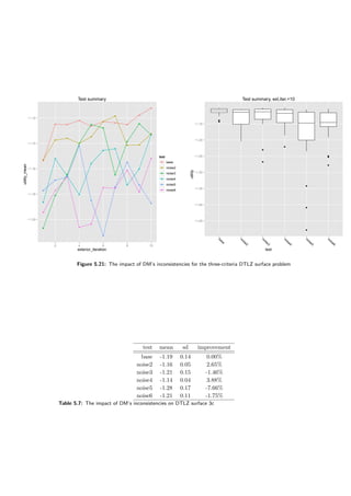
base 29236.10 355.30 0.00% -1.19 0.14 0.00%
generation45 29923.32 263.40 2.35% -1.17 0.08 -1.73%
generation60 30412.27 225.15 4.02% -1.14 0.05 -4.61%
solution45 29642.44 362.47 1.39% -1.12 0.03 -5.71%
solution60 29681.42 489.78 1.52% -1.14 0.11 -4.11%
Table 5.4: Importance of base parameters
Algorithm 4 Simulated DM indicating “good” solutions
1: procedure SelectGoodSolutions(solutions, toSelect)
2: solutions — a list of solutions generated in the interior loop
3: toSelect — how many solutions should be marked as “good”
4: for all s ∈ solutions do
5: s.value ← SupposedUtilityFunction(s)
6: end for
7: solutions ← Sort(key=value, descending=True)
8: Sort solutions on descending supposed utility
9: return GetFirst(solutions, toSelect)
10: end procedure
and the toSelect parameter is set to 3 so always three solutions are marked as good. One can
influence the behavior of SelectGoodSolutions by changing the toSelect parameter. But this
is not enough to simulate human-made inconsistencies.
First, note that one do not have to always select the same number of solutions. In fact, this
is unrealistic because the decision maker will select as many solutions as he or she will think
are appropriate. To simulate this behavior an additional parameter was added — toSelectDelta.
Now the number of solutions to be selected are taken from [toSelect − toSelectDelta, toSelect +
toSelectDelta] with uniform distribution.
Furthermore, the human decision maker is fallible. He or she can make a wrong decision and
not select the best solutions according to the supposed utility function. Another parameter was
introduced to simulate this phenomenon — noiseLimit. After sorting the solutions on the basis of
the supposed utility value the individuals 1, 2, . . . , noiseLimit are shuffled. Supposing one wants to
select three solutions. If the noiseLimit parameter is set to 0 (the default) three best solutions will
be selected. However, if an experimenter sets the noiseLimit to 6, then 3 out of 6 best solutions
will be picked by random.
The noisy version of the algorithm 4 is shown below.
Algorithm 5 Simulated DM indicating “good” solutions
1: procedure NoisySelectGoodSolutions(solutions, toSelect, toSelectDelta, noiseLimit)
2: for all s ∈ solutions do
3: s.value ← SupposedUtilityFunction(s)
4: end for
5: solutions ← Sort(key=value, descending=True)
6: shuffled ← ShuffleFirst(solutions, noiseLimit)
7: toSelect ← RandomFromInterval(toSelect − toSelectDelta, toSelect + toSelectDelta)
8: return GetFirst(shuffled, toSelect )
9: end procedure
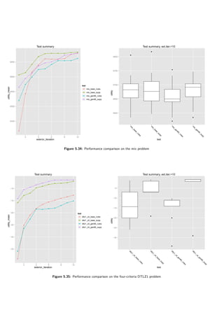
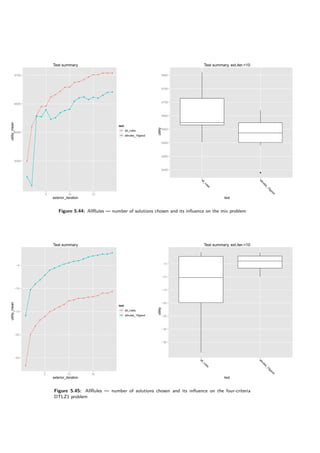
Following tests were performed:](https://image.slidesharecdn.com/4981f33e-4e84-4fb8-a033-f832840408ae-161203112639/85/igor-kupczynski-msc-put-thesis-58-320.jpg)
![60 5 Results of Computational Experiments
5.4.5 A different rule-generating algorithm
Details of a rule-generating algorithm is not part of the DARWIN specification. The choice of the
algorithm is left to the one implementing DARWIN. In this paper two approaches were evaluated
— the DomLem algorithm (see [16]) generating a minimal set of rules and the AllRules algorithm
(see [17]) generating an extensive set of all rules.
One can lower confidence of the rules generated in the DomLem algorithm (compare with 2.3).
100% confidence may seem a good idea; however, lowering it would allow more gradual improve-
ments of the goal function in the evolutionary algorithm which could lead to better results. Values
60% and 80% were tested. In the tests conducted earlier it was assumed that the decision maker
selects only a few solutions. In this section it is also compared with marking half of the solutions
as good.
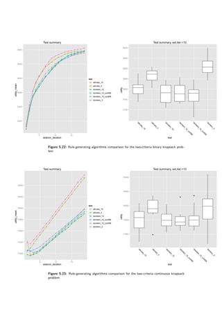
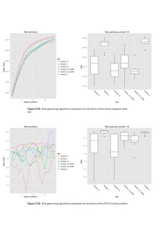
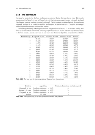
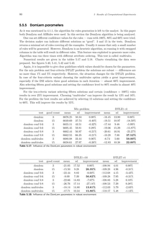
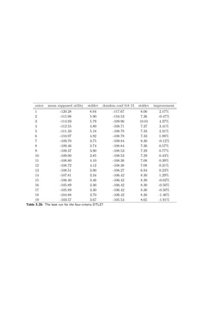
The results are presented in tables 5.8 and 5.9 and figures 5.22, 5.23, 5.24 and 5.25. When no
uncertainty is considered, DomLem performs better than AllRules and it is better to select three
solutions than fifteen — a half. Confidence however yields an interesting result — the algorithm
is robust with respect to confidence.
Knapsack bin 2c Knapsack cont 2c
algorithm good count mean sd improvement mean sd improvement
domlem 3 3909.94 47.17 0.00% 17939.27 700.25 0.00%
domlem 15 3773.55 53.12 -3.49% 17487.98 302.36 -2.52%
domlem conf 0.6 15 3783.62 46.17 -3.23% 17505.49 334.11 -2.42%
domlem conf 0.8 15 3764.69 58.01 -3.71% 17555.32 402.22 -2.14%
allrules 3 3865.25 31.93 -1.14% 17886.14 392.01 -0.30%
allrules 15 3804.01 43.96 -2.71% 17517.90 419.92 -2.35%
Table 5.8: Impact of the rule-generating algorithm on DARWIN
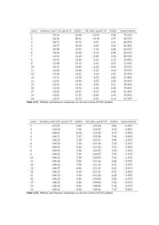
Knapsack bin 3c Surface 3c
algorithm good count mean sd improvement mean sd improvement
domlem 3 29282.28 227.33 0.00% -1.22 0.13 0.00%
domlem 15 27789.61 538.01 -5.10% -1.25 0.11 3.00%
domlem conf 0.6 15 28161.34 610.84 -3.83% -1.20 0.10 -1.02%
domlem conf 0.8 15 27775.05 336.66 -5.15% -1.21 0.14 -0.17%
allrules 3 29144.99 293.66 -0.47% -1.13 0.04 -7.47%
allrules 15 27979.16 772.90 -4.45% -1.24 0.11 1.73%
Table 5.9: Impact of the rule-generating algorithm on DARWIN](https://image.slidesharecdn.com/4981f33e-4e84-4fb8-a033-f832840408ae-161203112639/85/igor-kupczynski-msc-put-thesis-62-320.jpg)


![5.6 Conclusions 95
5.6 Conclusions
The experiments performed confirmed that the DARWIN method proposed in [13, 15, 9] is a good
too for solving multi-objective optimization problems even when the problem formulation does
contain uncertainty in the form of intervals of possible values.
The presented implementation is the first implementation of the DARWIN method which per-
mits performing so large computational experiments. The first task was to analyze behavior of
the algorithm on simple two-criteria problem without uncertainty. First evaluations allowed the
author to learn the properties and to get to know the behavior of the algorithm.
Having confidence that the DARWIN works it was possible to advance to the next task — to
evaluate the performance of a richer set of the problem. It was decided to start without allowing
uncertainty. Rationale behind this behavior was to prove the algorithm can solve a category of
problems with the good overall performance. Ignoring the uncertainty it was possible to compare
the DARWIN results with optimal ones, calculated by the linear programming solver.
There are a lot of parameters in the algorithm itself, so the next logical step was to check the
importance of the parameters. Experiments performed so far assumed that the decision maker
is infallible, consistent and acts according to a well-defined utility function. It is not the case in
real-life situations so the impact of inconsistencies in DM’s decisions was measured.
Knowing the characteristics, performance and impact of the parameters and the inconsistent
DM’s decisions one can check if the algorithm with similar characteristics on problems with interval
coefficients. Being unsatisfied with the performance on DTLZ1 problems the author checked the
influence of DomLem parameters on the result and included a second rules generating algorithm
— the AllRules algorithm. As a result a rich set of data containing performance characteristics
was gathered.
To conclude, the DARWIN method can handle very well a large variety of MOO problems.
A resulting solution is robust with respect to algorithm parameters, inconsistencies in Decision
Maker’s choices and finally to the uncertainty in the problem definition. Nevertheless the analyst
should be careful and investigate the problem instead of using the method blindly. There are some
problems which are hard for DARWIN to solve (e.g. DTLZ1). Even for these problems satisfactory
results can be achieved, however, one has to fine-tune the parameters and carefully observe their
impact on the result.
The method is simple to use for the decision maker even if he or she has no knowledge in the
decision support field. However for some problems the analyst’s assistance may be necessary in
order to select appropriate values for the parameters.](https://image.slidesharecdn.com/4981f33e-4e84-4fb8-a033-f832840408ae-161203112639/85/igor-kupczynski-msc-put-thesis-97-320.jpg)

![Chapter 6
Summary
In the paper a novel approach to multi-objective optimization was presented. The DARWIN
method is an interactive procedure utilizing the evolutionary algorithm to optimize a population
of solutions. The idea of DARWIN was first proposed by Salvatore Greco, Benedetto Matarazzo
and Roman Slowi´nski in [13, 15, 9]. However, in this paper the first implementation and numerical
results are provided.
The novelty of the method consists in utilizing an IMO process along with the EMO procedure.
DARWIN not only optimizes the population of solutions, but also drives the optimization towards
regions preferred by the decision maker. In order to do it, the preference information has to be
gathered. This is done by asking the DM a series of simple questions. A list of feasible solutions
is given and he or she is asked to indicate the “good” ones among them. The procedure uses
dominance-based rough set approach and the DomLem or AllRules algorithms to obtain a set of
“if . . . , then . . . ” decision rules. DARWIN is a first MOO technique using the decision rules.
The condition part of each rule corresponds to a dominance cone in the objective space built on
a subset of objectives. If a given solution matches the conditional part of the rule, it is considered
“good” with respect to this rule. The higher the number of rules matched, the higher the fitness
score in the evolutionary optimization, thus the bigger the chance to “survive” and advance to
the next generation.
DARWIN allows one to use intervals of possible values in the problem formulation. Multiple
scenarios are then tested. Objective space is transformed — it is no longer possible to provide
a value of an objective. One has to reason in terms of meaningful quantiles of each of the objectives.
This allows to take into account the decision maker’s attitude towards risk.
Two characteristics of the DARWIN method ensure robustness of the generated solutions.
Firstly, each solution is tested on multiple scenarios of uncertainty, so its characteristics are known
even considering fluctuations in the problem parameters. Secondly, the decision rules generated
by the DRSA framework are immune to inconsistencies in the decision maker’s choices. Therefore,
the algorithm can withstand inconsistencies in his or her decision and still guide the search towards
the preferred regions.
Performed computational experiments confirm the author’s intuition that the method can be
used to solve a class of multi-objective optimization problems. If there is no uncertainty involved
— the exact values of all problem coefficients are known — the resulting solutions are not further
than 10% from the optimal one. If the uncertainty is allowed a comparison to the optimal solution
is impossible, because it can not be provided to the problem that is not well-defined. However,
a comparison of the evolutionary optimization based on the DRSA decision rules with the one
where the supposed utility function is used can be made. The behavior of both optimizations is
similar and the conclusion is that the preference information extracted from the DM guides the
algorithm to the same regions where the supposed utility optimization. The results also showed
that DARWIN is immune to changes in parameters and, moreover, to inconsistencies in the decision](https://image.slidesharecdn.com/4981f33e-4e84-4fb8-a033-f832840408ae-161203112639/85/igor-kupczynski-msc-put-thesis-99-320.jpg)
![Bibliography
[1] Cormen, T. H., Leiserson, C. E., Rivest, R. L., and Stein, C. Introduction to Al-
gorithms. No. 35.2. MIT Press and McGraw-Hill, 2001, ch. The traveling-salesman problem,
pp. 1027–1033.
[2] Darwin, C. On the origin of species. John Murray, London, 1859.
[3] Deb, K. Introduction to Evolutionary Multiobjective Optimization. 59–96.
[4] Deb, K., Agrawal, S., Pratap, A., and Meyarivan, T. A Fast Elitist Non-dominated
Sorting Genetic Algorithm for Multi-objective Optimisation: NSGA-II. In PPSN VI: Proceed-
ings of the 6th International Conference on Parallel Problem Solving from Nature (London,
UK, 2000), Springer-Verlag, pp. 849–858.
[5] Deb, K., Thiele, L., Laumanns, M., and Zitzler, E. Scalable multi-objective opti-
mization test problems. In in Congress on Evolutionary Computation (CEC’2002 (2002),
pp. 825–830.
[6] Fogel, L. J. On the organization of intellect. PhD thesis, University of California, Los
Angeles, 1964.
[7] Goldberg, D. E. Genetic Algorithms in Search, Optimization and Machine Learning.
Addison-Wesley Longman Publishing Co., Inc., Boston, MA, USA, 1989.
[8] Graham, R. L., and Hell, P. On the history of the minimum spanning tree problem.
IEEE Ann. Hist. Comput. 7, 1 (1985), 43–57.
[9] Greco, S., Matarazzo, B., and Slowi´nski, R. DARWIN-PCT: Dominance-based rough
set Approach to handling Robust Winning solutionsin IN teractive multiobjective optimiza-
tion using Pairwise Comparison Tables. In Proceedings of the 25th Mini-EURO Conference
on Uncertainty and Robustness in Planning and Decision Making, URPDM 2010 (Coimbra,
Portugal, 15-17 April 2010).
[10] Greco, S., Matarazzo, B., and Slowi´nski, R. Rough sets theory for multicriteria deci-
sion analysis. European Journal of Operational Research 1, 129 (1 2001), 1–47.
[11] Greco, S., Matarazzo, B., and Slowi´nski, R. Handbook of Data Mining and Knowl-
edge Discovery. Oxford University Press, New York, 2002, ch. Multicriteria classification by
dominance-based rough set approach.
[12] Greco, S., Matarazzo, B., and Slowi´nski, R. Search Methodologies: Introductory Tu-
torials in Optimization and Decision Support Techniques. Springer-Verlag, New York, 2005,
ch. Rough set based decision support.](https://image.slidesharecdn.com/4981f33e-4e84-4fb8-a033-f832840408ae-161203112639/85/igor-kupczynski-msc-put-thesis-101-320.jpg)
![100 Bibliography
[13] Greco, S., Matarazzo, B., and Slowi´nski, R. Preferences and Decisions: Models and
Applications. Springer, Berlin, 2010 (to appear), ch. Dominance-based Rough Set Approach
to Interactive Evolutionary Multiobjective Optimization.
[14] Greco, S., Matarazzo, B., and Slowi´nski, R. DARWIN: Dominance-based rough set
Approach to handling Robust Winning solutions in INteractive multiobjective optimization.
In Proc. 5th International Workshop on Preferences and Decisions (Trento, April 6-8, 2009),
pp. 34–41.
[15] Greco, S., Matarazzo, B., and Slowi´nski, R. Interactive Evolutionary Multiobjective
Optimization using Dominance-based Rough Set Approach. In Proc. WCCI 2010, IEEE World
Congress on Computational Intelligence (Barcelona, Spain, July, 18-23, 2010), pp. 3026–3033.
[16] Greco, S., Matarazzo, B., Slowi´nski, R., and Stefanowski, J. An Algorithm for
Induction of Decision Rules Consistent with the Dominance Principle. In RSCTC ’00: Re-
vised Papers from the Second International Conference on Rough Sets and Current Trends in
Computing (London, UK, 2001), Springer-Verlag, pp. 304–313.
[17] Greco, S., Matarazzo, B., Slowi´nski, R., and Stefanowski, J. Variable consistency
model of dominance-based rough sets approach. In RSCTC ’00: Revised Papers from the
Second International Conference on Rough Sets and Current Trends in Computing (London,
UK, 2001), Springer-Verlag, pp. 170–181.
[18] Harrah, M. A build tool for Scala.
[19] Horn, A. On sentences which are true of direct unions of algebras. Journal of Symbolic
Logic, 16 (1951), 14–21.
[20] Keen, K. J. Graphics for Statistics and Data Analysis with R. Chapman & Hall/CRC, 2010.
[21] King, P., Naughton, P., DeMoney, M., Kanerva, J., Walrath, K., and Hommel,
S. Code Conventions for the Java Programming Language.
[22] Lazenby, D. Cygwin: For Windows NT. Linux J., 14.
[23] Lindholm, T., and Yellin, F. Java Virtual Machine Specification. Addison-Wesley Long-
man Publishing Co., Inc., Boston, MA, USA, 1999.
[24] Loeliger, J. Version Control with Git: Powerful Tools and Techniques for Collaborative
Software Development. O’Reilly Media, Inc., 2009.
[25] Metropolis, N. The beginning of the Monte Carlo method. Los Alamos Science Special
Issue dedicated to Stanislaw Ulam (1987), 125–130.
[26] Miettinen, K., Ruiz, F., and Wierzbicki, A. P. Introduction to Multiobjective Opti-
mization: Interactive Approaches. 27–57.
[27] Pawlak, Z. Rough sets. International Journal of Computer and Information Sciences 11
(1982), 341–356. 10.1007/BF01001956.
[28] Puchinger, J., Raidl, G. R., and Pferschy, U. The multidimensional knapsack problem:
Structure and algorithms. INFORMS J. on Computing 22, 2 (2010), 250–265.
[29] Rechenberg, I. Evolutionsstrategie - Optimierung technischer Systeme nach Prinzipien der
biologischen Evolution. PhD thesis, Technical University of Berlin, 1965.
[30] Schwefel, H. P. Kybernetische Evolution als Strategie der experimentellen Forschung in
der Str¨omungstechnik. Master’s thesis, Technical University of Berlin, 1965.](https://image.slidesharecdn.com/4981f33e-4e84-4fb8-a033-f832840408ae-161203112639/85/igor-kupczynski-msc-put-thesis-102-320.jpg)
![Bibliography 101
[31] Shafranovich, Y. Common format and mime type for comma-separated values (csv) files.
Tech. Rep. RFC 4180, IETF, October 2005.
[32] Wickham, H. ggplot2: elegant graphics for data analysis. Springer New York, 2009.
[33] Wirth, N. What can we do about the unnecessary diversity of notation for syntactic defini-
tions? Commun. ACM 20, 11 (1977), 822–823.
[34] Wolpert, D. H., and Macready, W. G. No free lunch theorems for optimization. IEEE
TRANSACTIONS ON EVOLUTIONARY COMPUTATION 1, 1 (1997), 67–82.
[35] ˙Zurawski, M. Algorithms of induction of decision rules for multicriteria and multiattribute
decision problems. Master’s thesis, Poznan University of Technology, 2001.](https://image.slidesharecdn.com/4981f33e-4e84-4fb8-a033-f832840408ae-161203112639/85/igor-kupczynski-msc-put-thesis-103-320.jpg)


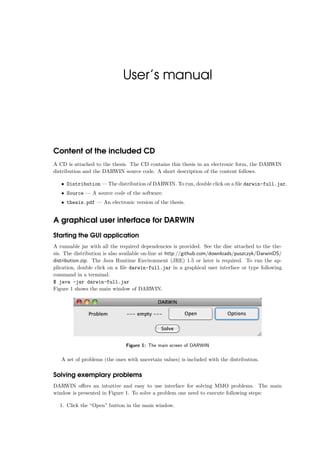
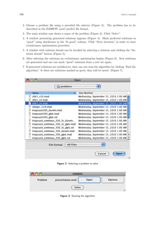
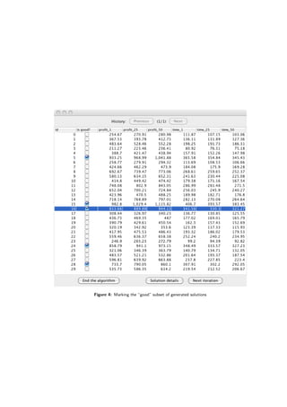
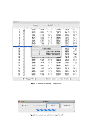
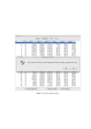
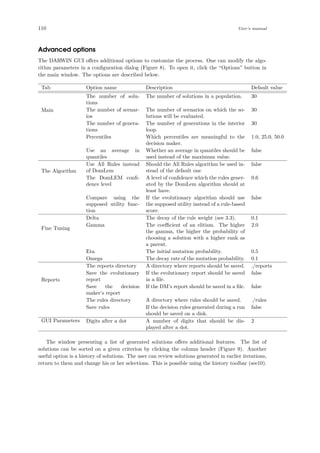
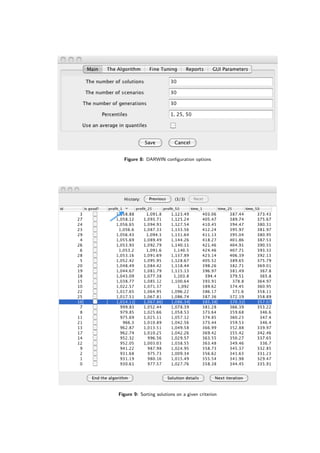
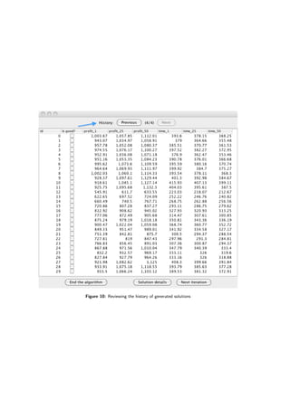
![The DARWIN .mod file format
MMO problems for DARWIN are specified in external files. These files are called the DARWIN
model files and usually have the .mod extension. The application contains a parser for the model
files. The parser grammar in the Extended Backus-Naur Form (EBNF, see [33]) is described below.
problem ::= { line }
line ::= statement , ";"
statement ::= utility_function |
variable |
goal |
constraint
variable ::= "var" , "[", [ var_type_constraint ], floating_point_number , ",",
floating_point_number ,
"]", identifier
var_type_constraint ::= "(B)" | "(I)"
goal ::= ("min" | "max"), identifier , ":", expression
constraint ::= identifier , ":", expression , (">=" | "<="), expression
utility_function ::= "!dec:", expression
expression ::= term , ("+" | "-"), expression |
term
term ::= factor , ("*" | "/"), term |
factor
factor ::= floating_point_number |
("+" | "-" | "ln"), factor |
quantile |
aggregate |
identifier |
interval |
"(", expression , ")"
quantile ::= "<", identifier , ",", floating_point_number , ">"](https://image.slidesharecdn.com/4981f33e-4e84-4fb8-a033-f832840408ae-161203112639/85/igor-kupczynski-msc-put-thesis-115-320.jpg)
![114 The DARWIN .mod file format
interval ::= "[", identifier , ":", floating_point_number , ",",
floating_point_number ,
"]"
aggregate ::= aggregate_operator , "(", expression , [{ ",", expression }], ")"
aggregate_operator ::= "sum" | "min" | "cos"
floating_point_number ::= ? A floating point number with an optional sign ?
identifier ::= ? A valid Java identifier ?
Comments handled by a preprocessor are possible — (1) line comments, starting with #, e.g.
#a-line-comment and (2) block comments, enclosed in /* */. Whitespaces are ignored.
A problem file consists of lines, each line contains a statement ended by a semicolon (;).
A statement can define the supposed utility function, a variable, a goal or a constraint. The
variables are defining the problem domain. They can be continuous (with double floating point
precision), binary (indicated by a (B) flag) or integer ((I) flag). Upper and lower limits of the
variable value have to be provided. Each variable has a name and can be referred by the name in
succeeding statements. Goals are the optimization criteria to be minimized or maximized. They
are named expressions and therefore can be referred later by the name. Constraints are named
inequalities. The inequality is not strict and both its sides can be expressions. Finally, the supposed
utility function is an expression prefixed with !dec:. The function is useful only if one wants to
simulate the decision maker.
An example file with the mix-problem definition is included below.
var[0, 13] xa;
var[0, 25] xb;
var[0, 13] xc;
max profit: [pa:20, 24] * min(xa , [da:10, 12])
+ [pb:30, 36] * min(xb , [db:20, 24])
+ [pc:25, 30] * min(xc , [dc:10, 12])
- [p1r:6, 7.2] * ([r1a:1, 1.2]* xa + [r1b:2, 2.4]* xb + [r1c :0.75 , 0.9]* xc)
- [p2r:9, 9.6] * ([r2a :0.5, 0.6]* xa + [r2b:1, 1.2]* xb + [r2c :0.5, 0.6]* xc);
min time: [ta:5, 6]*xa + [tb:8, 9.6]* xb + [tc:10, 12]* xc;
c1: xa <= 12;
c2: xb <= 24;
c3: xc <= 12;
c4: xa >= 0;
c5: xb >= 0;
c6: xc >= 0;
!dec: <profit , 0.01> + 3 * <profit , 0.25> + 2 * <profit , 0.50>
-1 * <time , 0.01> - 3 * <time , 0.25> - 2 * <time , 0.50 >;
The expressions are utilizing intervals (e.g. [pa:20, 24]) and the supposed utility function is
using meaningful percentiles (e.g. profit25%
: <profit, 0.25>).](https://image.slidesharecdn.com/4981f33e-4e84-4fb8-a033-f832840408ae-161203112639/85/igor-kupczynski-msc-put-thesis-116-320.jpg)
![Compiling DARWIN from the source
code
It is possible to build a DARWIN binary from the source code. It can be done using command
line on Windows, Linux and MacOSX. Instructions are given below.
1. Get the source code. Sources are included in a disk attached to the thesis. Alternatively,
most recent version is stored in the git repository (see [24]) and can be cloned by typing
a command:
$ git clone git://github.com/puszczyk/DarwinDS.git
2. Prepare a build tool. DARWIN uses sbt (see [18])— a build tool for Scala. Detailed setup
instructions are given in the project’s webpage. The easiest way is to install Scala (system-
dependent, consult http://scala-lang.org for details) and then prepare a script for running
sbt. Download sbt-launch.jar from the sbt website: http://simple-build-tool.googlecode.com/
files/sbt-launch-0.7.4.jar
Somewhere in the PATH put a script with the following content:
java -Xmx512M -jar ‘dirname $0‘/sbt-launch.jar "$@"
or (in case of Windows operating system):
set SCRIPT DIR=% dp0
java -Xmx512M -jar "%SCRIPT DIR%sbt-launch.jar" %*
Make the file executable. It is assumed further, that the script is named sbt.
3. Build the DARWIN binaries. Source code is located in the Darwin directory. First get
required dependencies:
$ cd DarwinDS/Darwin
$ sbt
> download-jars
Then run a set of unit-test to check if everything went fine up to this point:
> test
This should end with a message:
[info] All tests PASSED.
[success] Successful.
Now DARWIN can be compiled:
> compile
And run:
> run
To create a .jar package type:
> package](https://image.slidesharecdn.com/4981f33e-4e84-4fb8-a033-f832840408ae-161203112639/85/igor-kupczynski-msc-put-thesis-117-320.jpg)
![116 Compiling DARWIN from the source code
This will generate DARWIN binaries in a subdirectory named target.
The experiment framework
Instead of a graphical user interface, DARWIN can be run in a console-based batch mode. This is
useful for running a set of experiments. The batch run can be invoked by the experiment framework
located in the Experiment directory. The directory contains a few useful scripts written in Bash
and Python. As such it requirers MacOSX or a Linux distribution or a Windows operating system
with Cygwin installed (see [22]). The utility scripts are described below:
• runTestPlan.py — a script for running a set of tests. As an input it requires a location of the
DARWIN directory, a problem file, a darwin configuration file and a test plan specification.
The problem file is a file in the DARWIN .mod file format. The configuration is an .ini file
structured as follows:
[section]
option1 = value1
option2 = value2
(...)
optionN = valueN
Required sections and options are described in Table 4.1. The test plan specification is a
text file with the following structure:
>test_name_1/number -of -runs
[section -to -override]
option -to -override1 = value1
(...)
>test_name_N/number -of -runs
(...)
Each test is run number-of-runs times. For each test one can specify a list of options to
be overridden. It is useful for testing an influence of a parameter. An example test plan is
presented below.
>delta005 /15
[main]
delta = 0.05
>delta015 /15
[main]
delta = 0.15
>delta020 /15
[main]
delta = 0.20
>delta040 /15
[main]
delta = 0.40
This plan will run DARWIN fifteen times for each delta value. Run reports are saved in
a directory named after the current date and time. Test names are the names of subdirecto-
ries.
• genCharts.sh — a script for charting run reports. It requires installing the R environment
(see [20]) with ggplot2 and reshape libraries. The charts to be generated are included in](https://image.slidesharecdn.com/4981f33e-4e84-4fb8-a033-f832840408ae-161203112639/85/igor-kupczynski-msc-put-thesis-118-320.jpg)


![[IJCT-V3I2P31] Authors: Amarbir Singh](https://cdn.slidesharecdn.com/ss_thumbnails/ijct-v3i2p31-160609071410-thumbnail.jpg?width=640&height=640&fit=bounds)


